Stochastic modelling of the hydrogeological environment in low permeability sediment

Texte intégral

(1)STOCHASTIC MODELING OF THE HYDROGEOLOGICAL ENVIRONMENT IN A LOW PERMEABILITY SEDIMENT M. Huysmans1, A. Berckmans2, L. Feyen1,3 and A. Dassargues1,4 Hydrogeology & Engineering Geology Group, Department of Geology-Geograpy, Katholieke Universiteit Leuven, Belgium; [email protected] 2 ONDRAF/NIRAS, Brussel, Belgium 3 Stanford Hydrogeology Group, Department of Geological and Environmental Sciences, School of Earth Sciences, Stanford University 4 Hydrogeology, Department of Georesources, Geotechnologies and Building Materials, Université de Liège, Belgium 1. Abstract In Belgium, the Boom Clay is being considered as a potential host formation for the disposal of nuclear waste. Part of the safety assessment and feasibility studies of a potential nuclear waste disposal consists of hydrogeological modeling. In order to model the groundwater flow and possible radionuclide transport in the clay, the spatial distribution of the hydraulic conductivity of the clay has to be assessed. In this study, geostatistical methods are used to characterize the hydraulic conductivity field. More specific, direct sequential simulation of the hydraulic conductivity is carried out, using measurements of hydraulic conductivity and 4 types of soft data or secondary variables: resistivity logs, gamma ray logs, grain size measurements and descriptions of the lithology. The primary and secondary information is analyzed with geostatistical tools and combined to generate 100 fields of the hydraulic conductivity of the Boom Clay. Next, each field is input to a groundwater flow model to predict the advective travel time of constituents released from the disposed waste in the Boom Clay to the aquifers surrounding the Boom Clay. Statistical analysis of the ensemble of model predictions results in a predictive distribution for the advective travel time. This distribution reflects the uncertainty of the advective travel time that results from the uncertainty of the spatial distribution of the hydraulic conductivity of the Boom Clay.. Introduction The Belgian nuclear repository program, conducted by ONDRAF/NIRAS (Belgian agency for radioactive waste and enriched fissile materials) is in the process of characterizing the host rock capacities of the Boom Clay. The research activities are concentrated at SCK●CEN (Belgian Nuclear Research Centre) located on the nuclear zone of Mol/Dessel (province of Antwerp) where an underground experimental facility (HADESURF) was built in the Boom Clay at 225 m depth. In this area, the Boom Clay has a thickness of about 100 m and is overlain by some 180 m of water bearing sand formations. The Boom Clay is a marine sediment of Tertiary age (Rupelian), showing a distinct horizontal internal layering (Wouters & Vandenberghe, 1994). The isolation of the waste from the biosphere is obtained by means of a multi-barrier concept, composed of engineered and natural barriers. The performance of the disposal system as a whole is the most important aspect, but the evaluation of the various safety functions can offer added insights into the functioning of the disposal system and into its overall safety (SAFIR 2, 2001). Therefore hydrogeological studies must be carried out to determine the potential migration of radionuclides by the groundwater. It is however not easy to model the hydrogeology of low permeability environments. Several problems or difficulties occur. A first difficulty is the large effect of heterogeneities, such as sand or silt layers, on the groundwater movement and the transport. A second problem is the difficulty to measure hydraulic conductivity values and hydraulic heads in low permeability environments. Consequently, it is particularly interesting to include secondary data, such as resistivity, gamma ray, grain size and lithology. The aim of this study is to develop a methodology for modeling the hydrogeological conditions of low permeability sediments, taking into account the effect of geological heterogeneities on groundwater flow and solute transport. The method should make use of the available information of secondary or soft data. The method is applied on the Boom Clay..

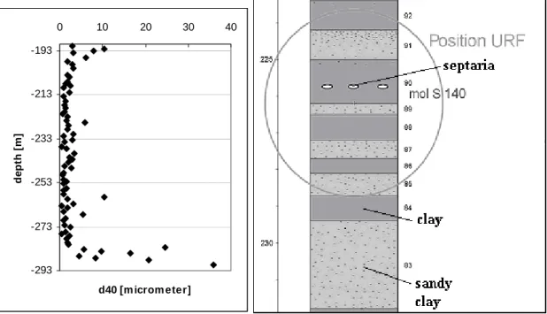
(2) Method The chosen method is based on geostatistical techniques because a variety of geostatistical tools exists to characterize and simulate heterogeneities and to incorporate secondary information. The first step is to collect and analyze the available hydraulic conductivity (K) measurements. All the measurements available for this study were carried out in the Mol-1 borehole (Wemaere et al., 2002). The information used is therefore one-dimensional. This is not a problem since the Boom Clay shows a distinct internal layering with a large lateral continuity. Correlation of several key horizons of the Boom Clay is possible between the Mol-1 borehole and the clay pits at a distance of more than 50 km (Wouters and Vandenberghe, 1994). Therefore it can be assumed that at a local scale the vertical variation of the hydraulic conductivity is the most important variability to be studied. Figure 1 shows the 52 vertical hydraulic conductivity measurements of the Boom Clay in the Mol-1 borehole. The log10 hydraulic conductivity values have a mean of -11.56 and a standard deviation of 0.41. The figure shows that in the Boom Clay three zones can be distinguished: an upper zone with a large variability of K (Transition Zone: 190.4m – 216m), a middle zone with a small variability of K (Putte and Terhagen Member: 216m – 278m) and the deepest zone with again a large variability of K (Belsele-Waas Member: 278m – 292.4m). The spatial structure of the hydraulic conductivity data in the vertical direction is studied by determining the variogram of the Kv-values in each of the three zones. The experimental and the modeled variograms of the Belsele-Waas Member e.g. are shown in Figure 2. The largest difference between the variograms of the three different zones is the difference of the total sill (the sum of the nugget and the sill): 0.065 in the Transition Zone, 0.019 in the Putte and Terhagen Member and 0.59 in the Belsele-Waas Member. This is a logical result since the largest variability of both the hydraulic conductivity and the different secondary variables occurs in the Belsele-Waas Member, while the values of K and the secondary variables have the lowest variance in the Putte and Terhagen Member. The range of the K variogram of the three units varies between 2.8m (Putte and Terhagen Member) and 12.3m (Transition Zone). The next step consists in collecting and analyzing the secondary variables. The measured variables available in this study are electrical resistivity, gamma ray, grain size and lithology, respectively shown in Figures 4, 5, 6 and 7. The electrical resistivity shows a clear correlation with the hydraulic conductivity: higher values of the resistivity correspond to higher values of the hydraulic conductivity. The correlation coefficient between hydraulic conductivity and resistivity is 0.73. Between the gamma ray measurements and the hydraulic conductivity values, the correlation coefficient is -0.65. This lower correlation is caused by the presence of organic matter and glauconite. The grain size is well correlated with the hydraulic conductivity. The correlation coefficient between d40, the grain size than which 40% is finer by weight, and the hydraulic conductivity is 0.95. The lithostratigraphic column, determined on the basis of a Formation Micro Imager (FMI) log (Mertens and Wouters, 2003), also shows a relationship with the hydraulic conductivity values: the mean log hydraulic conductivity of the clay layers (-11.7) is smaller than the mean log hydraulic conductivity of the silt layers (-11.3). This last secondary variable has a qualitative nature. It is coded to obtain numerical data, which can more easily be included in a geostatistical approach: clay = 1, sandy clay = 2, clayey sand = 3 and sand =4. The spatial structure of the secondary variables in every zone is also investigated. The variogram of each secondary variable is calculated and modeled. For every combination of 2 variables, the cross-variogram is calculated and modeled. An example is shown in Figure 3: this figure shows the experimental and the modeled cross-variogram of the gamma ray and the resistivity in the Belsele-Waas Member. All the spatial information is then used to perform co-kriging and co-simulation. The method to calculate the simulations is based on direct sequential simulation with histogram reproduction (DSSIM-HR) (Oz et al., 2003). This approach creates realizations that reproduce the (1) local point and block data in the original data units, (2) the mean, variance and variogram of the variable and (3) the histogram of the variable. The difference between the method described by Oz et al, and the method used in this study, is that for this study the algorithm is adapted to make it possible to take secondary variables into account. This is done by replacing the simple kriging step by a simple co-kriging step. In this way, the estimated value and the variance calculated in the kriging step are also dependent on the neighbouring secondary data measurements,.

(3) and not only on the neighbouring K measurements. Figure 8 shows the results of the co-kriging of the vertical hydraulic conductivity of the Boom Clay using measurements of the hydraulic conductivity, the resistivity, the gamma ray, the grain size and the lithology. This figure clearly shows the effect of dividing the Boom Clay into three zones with a different spatial structure. As expected from the variogram models, the variability of the estimated hydraulic conductivity in the Belsele-Waas Member and the Transition Zone is much larger than in the Putte and Terhagen Member. Figure 9 shows one result of 100 equiprobable direct sequential simulation realizations of the vertical hydraulic conductivity of the Boom Clay using the same measurements. It is clear that the conditional simulation results show a much larger variability than the co-kriging results. Since direct sequential simulation reproduces the variogram, it can be expected that this higher variability is more realistic for the Boom Clay than the limited variability of the K values estimated by co-kriging. Next, each of the 100 equiprobable hydraulic conductivity fields is introduced as input for a simple 1D vertical groundwater flow model. The Boom Clay is assumed to be horizontally layered and the flow is assumed to be in the vertical direction only. The downward vertical hydraulic gradient is 0.02. The waste disposal galleries are assumed to be in the middle of the Boom Clay layer. This groundwater model enables to make a prediction of the advective travel time of solutes derived from the potential waste galleries in the Boom Clay to the aquifers surrounding the Boom Clay.. Results Statistical analysis of the ensemble of model predictions results in a predictive distribution for the advective travel time. This distribution reflects the uncertainty of the advective travel time that results from the uncertainty of the spatial distribution of the hydraulic conductivity of the Boom Clay. This distribution is shown in Figure 10. Taking secondary data into account, the mean advective travel time is 392592 years and the standard deviation is 14176 years. The advective travel time distribution based on simulations that include secondary information is compared with the advective travel time distribution that does not include secondary information. This latter distribution is shown in Figure 11. The mean advective travel time is 367628 year and the standard deviation is 9419 year. Including the secondary data thus increases the mean advective travel time with 7.5% and increases the standard deviation with 51%. Therefore, including the secondary data leads to larger values of the advective travel time with a larger variance. This effect can easily be explained. Including the secondary data leads to a higher variability of the simulated hydraulic conductivity values. Therefore more low permeability peaks occur in the vertical variation of K in the Boom Clay. Since the advection is modeled as 1D vertical in a horizontally layered model, the effective hydraulic conductivity of the medium is the harmonic mean of the simulated K values. The harmonic mean decreases considerably when low permeability extremes are present. Since the use of secondary data leads to more low permeability peaks, the effective K decreases and therefore the advective travel time which is inversely proportional with the effective hydraulic conductivity, increases.. Conclusion In this study, direct sequential simulations were used to model the hydrogeological conditions of the Boom Clay, taking into account the presence of geological heterogeneities and using the information of secondary data. A large number of simulations was generated and used as input hydraulic conductivity fields in a groundwater flow model, in order to obtain a distribution of the advective travel time of solutes in the Boom Clay. Two important conclusions can be drawn from the results of these calculations. First, dividing the area in three zones with a different spatial structure has an important effect on the local variability of the simulated fields. The authors believe that this division leads to more realistic hydraulic conductivity simulations. Secondly, including secondary data leads to a different advective travel time distribution than if this information is not used. This secondary information thus holds the potential to improve the estimation and simulation of hydraulic conductivity..

(4) Figures. Figure 1. Hydraulic conductivity measurements of the Boom Clay in the Mol-1 borehole. Figure 2. The variogram of the log hydraulic conductivity of the Belsele-Waas Member in the vertical direction. Figure 3. The cross-variogram of the gamma ray and the resistivity in the Belsele-Waas Member in the vertical direction. 10. 0. 100. -193. -193. -213. -213. -233. -233. depth [m]. depth [m]. 1. -253. 50. 100. -253. -273. -273. -293. -293. Resistivity [ohm m ]. Figure 4. Resistivity of the Boom Clay in the Mol-1 borehole. Figure 5. Gamma ray of the Boom Clay in the Mol-1 borehole.. Gam m a ray [gAPI].

(5) 0. 10. 20. 30. 40. -193. depth [m]. -213. -233. -253. -273. -293 d40 [m icrom eter]. Figure 6. Grain size d40 of the Boom Clay in the Mol-1 borehole. Figure 7. Part of the lithostratigraphic column of the Boom Clay in the Mol-1 borehole (Mertens and Wouters, 2003). -11. -10. -9. -13. -11. -10. -9. -200. -200. -220. -220. -240. log K [m /s]. -12. depth [m]. -12. depth [m]. -13. -240. -260. -260. -280. -280. -300. -300 log K [m /s]. Figure 8. Co-kriging of the vertical hydraulic conductivity of the Boom Clay using measurements of the hydraulic conductivity, the resistivity, the gamma ray, the grain size and the lithology. Figure 9. Direct sequential simulation of the vertical hydraulic conductivity of the Boom Clay using measurements of the hydraulic conductivity, the resistivity, the gamma ray, the grain size and the lithology..

(6) Histogram. Histogram. 120.00%. 25. 100.00%. 20. 80.00%. 15. 60.00%. 10. 40.00%. 20.00%. 5. 20.00%. .00%. 0. .00%. 120.00%. 25. 15 60.00% 10 40.00% 5. 33 0 34 0 00 0 35 0 0 0 0 36 0 0 00 0 37 00 0 38 0 0 00 0 39 00 0 40 0 0 00 0 41 0 0 0 42 0 00 00 00. 0. Advective travel tim e [year]. 33 0 34 0 00 0 35 0 0 00 0 36 00 0 37 0 0 00 0 38 00 0 39 0 0 00 0 40 00 0 41 0 0 0 0 42 0 00 00 00. 80.00%. Frequency. 100.00%. 20 Frequency. 30. Advective travel tim e [year]. Figure 10. Advective travel time distribution taking hydraulic conductivity data and secondary data into account Figure 11. Advective travel time distribution taking only hydraulic conductivity data into account. Acknowledgements The authors wish to thank ONDRAF/ NIRAS (Belgium agency for radioactive waste and enriched fissile materials) and SCK-CEN (Belgian Nuclear Research Centre) for providing the necessary data for this study. The authors wish to acknowledge the Fund for Scientific Research – Flanders for providing a Research Assistant scholarship to the first author.. References Mertens, J. and Wouters, L., 2003, 3D Model of the Boom Clay around the HADES-URF, NIROND report 2003-02, 48 p. Oz, B., Deutsch, C. V., Tran, T. T. and Xie, Y., 2003, DSSIM-HR: A FORTRAN 90 program for direct sequential simulation with histogram reproduction: Computers & Geosciences, v. 29, no.1, p. 39-51. Wemaere, I., Marivoet, J., Labat, S., Beaufays, R. and Maes, T., 2002, Mol-1 borehole (April-May 1997): Core manipulations and determination of hydraulic conductivities in the laboratory, R-3590, 56 p. Wouters, L. and Vandenberghe, N., 1994, Geologie van de Kempen: een synthese: Niras, NIROND-94-11, Brussel, 208 p..

(7)