Indexation et recherche d’images par arbres des coupes

Texte intégral

(1)Indexation et recherche d’images par arbres des coupes Petra Bosilj. To cite this version: Petra Bosilj. Indexation et recherche d’images par arbres des coupes. Traitement des images [eess.IV]. Université de Bretagne Sud, 2016. Français. �NNT : 2016LORIS396�. �tel-01362165�. HAL Id: tel-01362165 https://tel.archives-ouvertes.fr/tel-01362165 Submitted on 4 Jan 2017. HAL is a multi-disciplinary open access archive for the deposit and dissemination of scientific research documents, whether they are published or not. The documents may come from teaching and research institutions in France or abroad, or from public or private research centers.. L’archive ouverte pluridisciplinaire HAL, est destinée au dépôt et à la diffusion de documents scientifiques de niveau recherche, publiés ou non, émanant des établissements d’enseignement et de recherche français ou étrangers, des laboratoires publics ou privés..

(2) THESE / UNIVERSITE DE BRETAGNE LOIRE sous le sceau de l'Université Bretagne Loire. présentée par : Petra Bosilj UMR 6074 Université Bretagne Loire. pour obtenir le titre de DOCTEUR DE L’UNIVERSITE DE BRETAGNE LOIRE Mention : Informatique. Institut de Recherche en Informatique et Systèmes Aléatoires. Ecole doctorale SICMA. Image indexing and retrieval using component trees. Thèse soutenue le 25 Janvier 2016 à Vannes devant le jury composé de :. Jiří Matas Professor, Czech Technical University in Prague // rapporteur. Philippe Salembier Professor, Universitat Politècnica de Catalunya // rapporteur. Jean-Marc Ogier Professeur, Université La Rochelle // examinateur. Michael H. F. Wilkinson Senior Lecturer / Associate Professor, University of Groningen // examinateur. Erchan Aptoula Associate Professor, Okan University // examinateur. Sébastien Lefèvre Professeur, Université de Bretagne-Sud, IRISA // directeur de thèse. Ewa Kijak Maître de Conférences, Université Rennes 1, IRISA // directeur de thèse. Image indexing with component trees Petra Bosilj 2016.

(3) Image indexing with component trees Petra Bosilj 2016.

(4) I would like to thank my advisors, Sébastien Lefèvre and Ewa Kijak, for all their guidance and advice. A special thanks to the reviewers whose comments have helped improve the manuscript, and all the collaborators I have worked with during my Ph. D. studies. I also want to express my gratitude to all my friends and especially my family, and all their support, understanding and encouragement that helped me keep my focus.. Image indexing with component trees Petra Bosilj 2016.


(6) i. Contents. 1 Introduction. 1. 1.1. Image Representations . . . . . . . . . . . . . . . . . . . . . . . . . . . . . . . .. 2. 1.2. Image Retrieval and Classification . . . . . . . . . . . . . . . . . . . . . . . . .. 5. 1.3. Contributions and Content . . . . . . . . . . . . . . . . . . . . . . . . . . . . . .. 6. 2 Formalization of Component Trees. 11. 2.1. Basic Notions . . . . . . . . . . . . . . . . . . . . . . . . . . . . . . . . . . . . .. 13. 2.2. Component Trees as Stackable Hierarchies of Regions . . . . . . . . . . . . . .. 17. 2.3. Categorization of Tree Representations into Superclasses . . . . . . . . . . . .. 19. 2.4. Indexing the SHoR . . . . . . . . . . . . . . . . . . . . . . . . . . . . . . . . . .. 21. 3 Overview of Component Trees. 27. 3.1. Min and Max-trees . . . . . . . . . . . . . . . . . . . . . . . . . . . . . . . . . .. 28. 3.2. Tree of Shapes . . . . . . . . . . . . . . . . . . . . . . . . . . . . . . . . . . . . .. 32. 3.2.1. Topological Tree of Shapes . . . . . . . . . . . . . . . . . . . . . . . . . .. 34. Binary Partition Tree . . . . . . . . . . . . . . . . . . . . . . . . . . . . . . . . .. 36. 3.3.1. Binary Partition Tree by Altitude Ordering . . . . . . . . . . . . . . . .. 39. 3.3.2. Hierarchies of Minimum Spanning Forests . . . . . . . . . . . . . . . .. 41. 3.4. α-tree . . . . . . . . . . . . . . . . . . . . . . . . . . . . . . . . . . . . . . . . . .. 45. 3.5. (ω )-tree . . . . . . . . . . . . . . . . . . . . . . . . . . . . . . . . . . . . . . . . .. 48. 3.6. Comparative summary . . . . . . . . . . . . . . . . . . . . . . . . . . . . . . . .. 51. 3.3. 4 Component Tree based Maximally Stable Regions. 57. 4.1. Salient Regions Detection . . . . . . . . . . . . . . . . . . . . . . . . . . . . . .. 58. 4.2. Maximally Stable Extremal Regions . . . . . . . . . . . . . . . . . . . . . . . .. 60. 4.3. Maximally Stable Regions from Component Trees . . . . . . . . . . . . . . . .. 64. 4.3.1. Maximally Stable Regions on Tree of Shapes . . . . . . . . . . . . . . .. 65. 4.3.2. Maximally Stable Regions on α-tree and (ω )-tree . . . . . . . . . . . .. 67. Image indexing with component trees Petra Bosilj 2016.

(7) ii. Contents. 5 Validation of Tree-MSR 5.1. 5.2. 71. Region Matching . . . . . . . . . . . . . . . . . . . . . . . . . . . . . . . . . . .. 72. 5.1.1. Evaluation Framework . . . . . . . . . . . . . . . . . . . . . . . . . . . .. 73. 5.1.2. Matching Results . . . . . . . . . . . . . . . . . . . . . . . . . . . . . . .. 76. Image Retrieval . . . . . . . . . . . . . . . . . . . . . . . . . . . . . . . . . . . .. 78. 5.2.1. Evaluation Framework . . . . . . . . . . . . . . . . . . . . . . . . . . . .. 80. 5.2.2. Image Retrieval Results . . . . . . . . . . . . . . . . . . . . . . . . . . .. 83. 6 Local Pattern Spectra. 87. 6.1. Feature Description . . . . . . . . . . . . . . . . . . . . . . . . . . . . . . . . . .. 88. 6.2. SIFT Descriptors . . . . . . . . . . . . . . . . . . . . . . . . . . . . . . . . . . . .. 88. 6.3. Pattern Spectra as Descriptors . . . . . . . . . . . . . . . . . . . . . . . . . . . .. 90. 6.3.1. Attributes and Filtering . . . . . . . . . . . . . . . . . . . . . . . . . . .. 90. 6.3.2. Size and Shape Granulometries . . . . . . . . . . . . . . . . . . . . . . .. 93. 6.3.3. Global Pattern Spectra . . . . . . . . . . . . . . . . . . . . . . . . . . . .. 94. 6.3.4. Local Pattern Spectra . . . . . . . . . . . . . . . . . . . . . . . . . . . . .. 96. 7 Descriptor Validation 7.1. 7.2. 7.3. 101. Image Classification . . . . . . . . . . . . . . . . . . . . . . . . . . . . . . . . . . 101 7.1.1. Database and Experimental Setup . . . . . . . . . . . . . . . . . . . . . 102. 7.1.2. Parameter Tuning . . . . . . . . . . . . . . . . . . . . . . . . . . . . . . . 106. 7.1.3. Results . . . . . . . . . . . . . . . . . . . . . . . . . . . . . . . . . . . . . 108. Satellite image retrieval . . . . . . . . . . . . . . . . . . . . . . . . . . . . . . . . 113 7.2.1. Dataset and Evaluation Metrics . . . . . . . . . . . . . . . . . . . . . . . 114. 7.2.2. Settings of Pattern Spectra Approaches . . . . . . . . . . . . . . . . . . 114. 7.2.3. Retrieval results . . . . . . . . . . . . . . . . . . . . . . . . . . . . . . . . 117. Discussion and Perspectives . . . . . . . . . . . . . . . . . . . . . . . . . . . . . 118. 8 Complexity Driven Tree Simplification. 121. 8.1. Premises of the Algorithm . . . . . . . . . . . . . . . . . . . . . . . . . . . . . . 122. 8.2. The Simplification Technique . . . . . . . . . . . . . . . . . . . . . . . . . . . . 123 8.2.1. 8.3. Complexity Analysis . . . . . . . . . . . . . . . . . . . . . . . . . . . . . 125. Proposed Applications . . . . . . . . . . . . . . . . . . . . . . . . . . . . . . . . 126. 9 Conclusions and Perspectives. 129. 9.1. Conclusions . . . . . . . . . . . . . . . . . . . . . . . . . . . . . . . . . . . . . . 129. 9.2. Perspectives in Image Retrieval . . . . . . . . . . . . . . . . . . . . . . . . . . . 131 9.2.1. Improvements to the Proposed Methods . . . . . . . . . . . . . . . . . 132. 9.2.2. A Step Further . . . . . . . . . . . . . . . . . . . . . . . . . . . . . . . . 133. Image indexing with component trees Petra Bosilj 2016.

(8) Contents 9.3. iii. Open Challenges on Component Trees . . . . . . . . . . . . . . . . . . . . . . . 134. Image indexing with component trees Petra Bosilj 2016.

(9) iv. Contents. Image indexing with component trees Petra Bosilj 2016.

(10) 1. Chapter. 1. Introduction. Contents 1.1. Image Representations . . . . . . . . . . . . . . . . . . . . . . . . . . . . . .. 2. 1.2. Image Retrieval and Classification . . . . . . . . . . . . . . . . . . . . . . . .. 5. 1.3. Contributions and Content . . . . . . . . . . . . . . . . . . . . . . . . . . . .. 6. The field of image processing belongs to the discipline of signal processing dealing with processing of analog and digital signal, as well as storing, filtering and performing other operations on those signals. While image processing can be further divided into analog and digital image processing, the focus of this thesis are the applications belonging to the digital image processing field. In digital image processing, the input signals are images represented as two-dimensional, discrete functions which can take on a finite range of values, representing the image intensity. The field of digital image processing refers to processing such signals with a digital computer [74]. While the related field of computer graphics is easy to distinguish from image processing, as it deals with the formation of images from object models as can be viewed as the “other side of the medal” to the image processing field, the boundary between image processing, image analysis and computer vision is somewhat less clear. A simple distinguishing criterion usually defines image processing operations to be those where both the input and output information are images. However, simple tasks such as computing the average intensity in an image would not be included in image processing under this definition [74]. The field of computer vision is usually considered to deal with more complex understanding tasks, with the goal of emulating human visions, learning and being able to. Image indexing with component trees Petra Bosilj 2016.

(11) Chapter 1 – Introduction. 2. take actions based on input. As such, there also exists an overlap with artificial intelligence as well as machine learning, as the techniques from these fields are used to achieve image understanding. While computer vision and image analysis tasks can be said to perform high-level processing on images where the goal is to “make sense” of the objects recognized in the image and perform cognitive functions associated with vision, we can define image processing as a field dealing with low-level and mid-level processing on images [74]. Here, the low-level processing involves primitive operations such as noise reducing preprocessing techniques, contrast enhancement and image sharpening. Mid-level processing then further processes the images, but typically outputs the attributes extracted from those images, such as a segmentation of the image into regions or objects, description of the objects as well as their classification. Image processing can thus be defined to encompass the processes whose inputs are images, and the outputs are either images or attributes extracted from the images (up to and including the recognition of individual objects) [74]. These methods work on images obtained by different acquisition techniques, such as X-ray imaging, satellite and radar imaging, as well as imaging in the visible and infrared bands, and includes processes such as image enhancement, image sharpening and restoration, image segmetation, representation and description as well as recognition and retrieval. In the next section, we present different representations used in image processing, ranging from the simplest pixel-based representations to complex representations suited for various specific image processing applications. Different representations are used for different specific application domains within the field and depend both on the nature of the images being processed as well as the intended application, and we focus in this work on hierarchical image representations. The chosen application domain, image retrieval (and the related domain of classification) is presented in Sec. 1.2 which gives a short overview of the general image retrieval systems (a more detailed introduction to image retrival is given later). Finally, Sec. 1.3 summarizes the contributions presented in the rest of the thesis and gives the overview of the organization of the manuscript.. 1.1 Image Representations Many different image representations exist and, according to their properties, are suited for different application domains. Accuracy of the representation, redundancies present, the size of the representation and the number of elements, as well as the relations between the elements of the representation all have to be considered. For example, if the goal is to store a large collection of images, a representation using as little memory as possible while still allowing for perfect image reconstruction would be preferable. On the other hand, if the. Image indexing with component trees Petra Bosilj 2016.

(12) 1.1 – Image Representations goal is to manipulate with the represented image, the size of the representation is not as important as the direct access to image data allowing for easy modification of the image. Here, we list several different families of image representations as well as their principal characteristics: • Pixel-based representation of an image is the simplest to define, with elements in sim-. ple neighboring relations [175] and containing only direct, uninterpreted intensity (or color) information. In contrast with the simplicity of this representation is a large number of elements to be examined with no previous interpretation of associated local information [158].. • Block-based representations divide the image into the set of (rectangular) arrays of pixels. Different block-based representations have been developed for both binary images [118, 67, 147] and grayscale images [215, 48, 47]. The number of elements is slightly reduced compared to pixel-based representation, but the representation still does not include any interpretation of image data. Most common application include image compression [48, 215, 118], segmentation [147, 215], sliding window techniques [92] and efficient extraction of various features and attributes from the images [47, 147, 67]. • Compressed domain (or frequency domain) representations store the image as a set of. coefficients in the transform domain. Different representations are based on Fourier transform [58, 200], wavelet theory [200, 103], Gabor wavelets [94], ridgelets [61], contourlets [60] etc. Some of typical uses of this representation include image compression [103, 200], denoising [104, 61], reconstruction [94] and texture analysis and segmentation for images [35]. While these representations reduce the size of the image, they are sensitive to translation, rotation and scaling of the image [119]. Additionally, in the frequency domain it is difficult to manipulate localized image content.. • Region-based representations differ from block-based in a way that regions are created by grouping similar and connected pixels, usually using a segmentation algorithm.. The algorithm used typically produces an over-segmentation and the resulting regions are often called superpixels [1]. Information about the region adjacency is kept, usually in a region-adjacency graph (RAG) [156] or combinatorial maps [97]. Different approaches to calculating the segmentation of the image into superpixels have been explored, e.g. normalized cuts [168], graph-based segmentation by Felzenszwalb and Huttenlocher [66] or different approaches to watershed segmentation [204,. Image indexing with component trees Petra Bosilj 2016. 3.

(13) Chapter 1 – Introduction. 4. (a). (b). Figure 1.1: The tree in (b) is an example of a hierarchical representation of (a) 52]. A comparison between different approaches to superpixel calculation is presented in [1]. The theory of segmentation and their mathematical properties were also studied in-depth by [165, 155]. The number of regions is reduced compared to pixel-based representations, while the representation accuracy can be kept [158]. Still, a generic method for automatic segmentation of an image into semantic objects remains an open question and in order to detect semantic structures (e.g. objects) in the data, different unions of multiple regions have to be considered [202]. • Hierarchical representations propose most likely unions of regions (of a region-based representation) on different scales of the image, storing fine image details as well as. coarse simplifications of images [202]. While they are built on (partial) segmentations, hierarchical representations hold more information than a simple collection of nested segmentations of an image. In addition to storing horizontal relations between regions (i.e. regions at the same level of detail), they also encode vertical relation between regions at different image scales which enable analysis of object details and provide the information on inclusion relations between the objects. The first applications were focused on image filtering and segmentation in the framework of Mathematical Morphology [88, 159, 158], and hierarchical representations are still used for this kind of applications [50, 178]. They bridge the gap between the classical filtering and segmentation techniques [161], enabling the construction of connected operators by simplifying different hierarchical representations. Various other applications have emerged since, such as object detection [202], video segmentation [159], image simplification [173, 120], feature extraction [136], image retrieval and classification [183, 182, 190, 9] and image registration [119]. An example of such an image decomposition is given in Fig. 1.1. More exhaustive list of applications is given later, according to hierarchy type (cf. Tab. 3.2). Hierarchical representations of images are in the focus of this work. Ever since emerging, these representations have aimed to find better ways to capture the semantic information. Image indexing with component trees Petra Bosilj 2016.

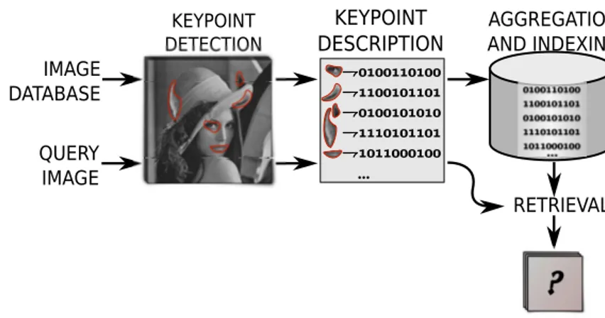
(14) 1.2 – Image Retrieval and Classification about the image and propose complex regions corresponding to “meaningful” objects (components) of the image [88, 159]. For this reason, the term component tree was used to describe first proposed hierarchical representations [88]. Recently, many different such hierarchical representations have been developed; Trees of Shapes [120, 184, 73], Binary Partition Trees [158, 202] and trees based on them (e.g. BPT by Altitude Ordering [51], Hierarchies of Minimum Spanning Forests [50]), α-trees [173, 142] and constrained connectivity hierarchies, such as (ω )-trees [173, 135] being some of them.. 1.2 Image Retrieval and Classification The validation of the work presented herein is done in image retrieval and classification, akin application fields from computer vision and image processing. While the goal of image retrieval is to retrieve the database images describing the same object or scene as the query, in image classification the previously known images have already been grouped into classes based on a common object or a scene they are describing and the query image is assigned to the appropriate class. This is typically achieved by means of computing a description of the image, known then as a global image descriptor [140, 195, 45, 206], a numerical representation of the image which can then be used to get a measure of image similarity. However, due to problems caused by occlusion, as well as objects in a scene belonging to different planes and thus behaving differently under various transformations (e.g. translation and rotation), descriptor schemes based on locally detected regions and features often tend to be more powerful [163]. The detection of distinctive, invariant and discriminative local features is used to provide a compact representation of the image by only focusing on the salient areas of the image. The development of affine invariant detectors was driven by their robustness against viewpoint change as one of the most common scene transformations between images. Popular detectors rely on different approaches to detect salient regions and points, operating in scale space or based on image gradient [99, 19, 115, 4, 14], relying on edges and boundaries [90, 198] or image and region contrast [108]. Detections returned by different detection approaches are often complementary and can be used in combination. Depending on the application and the type of content in the images under examination, predetermined parts of the image can also be selected as local features, covering the image in dense patches sometimes extracted from a regular rectangular grid covering the whole image (with or without overlap) [93, 189, 219, 146, 33]. After selecting or detecting features and keypoints locally, local description methods are applied to the detected salient points [99, 19, 189, 3] which are then aggregated and stored in an index. In small scale retrieval systems, as well as some application domains such as image matching or registration, all the local descriptors can be stored directly and searched. Image indexing with component trees Petra Bosilj 2016. 5.

(15) Chapter 1 – Introduction. 6 KEYPOINT DETECTION. IMAGE DATABASE. KEYPOINT DESCRIPTION. AGGREGATION AND INDEXING. +0100110100 +1100101101 +0100101010 +1110101101 +1011000100 .... QUERY IMAGE. RETRIEVAL. Figure 1.2: A representation of the main parts of the retrieval system based on a local approach. The steps of keypoint detection and description are performed for all the database images, after which the database descriptors are aggregated and stored in an index. For each new query image, the same steps of keypoint detection and description are first performed (the global query descriptor is also produced from the local ones if an aggregation step is included). Finally, index storing all the database descriptors is queried using the query descriptors to retrieve similar images from the database. through using (approximate) nearest-neighbor based techniques [124, 96, 56, 167]. However, due to the curse of dimensionality [24, 27], especially when constructing a large scale image retrieval or object recognition system, the descriptors are often first aggregated before being stored in an index [170, 86, 16]. While some loss of information is always present, aggregating local descriptors using a combination of an aggregation and an indexing scheme produces a singular global descriptor for every image thus providing again a simple and efficient way to compare the similarity between two images. A simple depiction of such a scheme is shown in Fig. 1.2. Using different indexing schemes facilitates performing large scale database search thus making it possible to handle a very large collection of local descriptors, as well as balance the effects of uneven number of selected features coming from different scenes due to the difference in the type of content they represent.. 1.3 Contributions and Content The motivation to employ these hierarchical image representations for the classification and retrieval tasks comes from the specific semantic information captured by such hierarchies, which enables us to work directly on a reduced search space organizing the potentially salient image regions according to their complexity level as well as their inclusion relations to other regions. This claim is supported by the previous applications of such features to retrieval and classification, ranging from simpler approaches working with predefined classes. Image indexing with component trees Petra Bosilj 2016.

(16) 1.3 – Contributions and Content [183, 182] to more recent approaches where the trees and other morphological tools are used to perform large scale retrieval on either general databases, or specific databases comprising microscopic or satellite data [195, 190, 7, 136]. The saliency of the regions contained in the representations was previously demonstrated on the earliest of hierarchical representations, when an alternate detection algorithm for MSER regions [108] was presented using the Min and Max-tree hierarchies [136] as they contain all the potential MSER candidates as their building blocks. The claim of saliency and robustness of the regions represented by the trees is further supported by their wide use for segmentation and object detection [159, 202, 22, 112, 186]. In addition to working with salient regions directly, hierarchical representations were used to aggregate identifying information about the components they contain, thus producing distinctive descriptors. While previously only used as parts of global description schemes [195, 190] as (global) Pattern Spectra as well as to describe images at the pixel-resolution using Differential Attribute Profiles (DAP)[22, 55, 141] and more general and robust Differential Morphological Profiles (DMP) [21], these applications prove that discriminative information throughout different scales of the image can be sucessfully accumulated from examining the building blocks of such hierarchies. Extending previous work exploiting hierarchical representations to construct different elements of the retrieval and classification systems, we present here several advances towards more versatile application of various component trees from mathematical morphology to these domains. The rest of the work presented herein is structured as follows: • Chapters 2 and 3 correspond to the morphological context of this thesis, offering an overview of different hierarchies present in the literature with the focus on explaining. and comparing their structural characteristics as well as efficiency of computation. In addition to offering an exhaustive survey of the state-of-the-art hierarchies in a context different from other published works concerned with multiple such representations, we propose a classification of such representations into two superclasses, which follows the same argumentation in the hierarchical case as the seminal work of Serra [165] and Ronse [155] defining the relations between the frameworks of segmentations and partial segmentations of images. Included in the examination and formalization of the hierarchies from a general perspective, as well as each of the superclasses, is also a way of indexing i.e. assigning measures of scale or coarseness to the components in a hierarchy. The standard way of visualizing the indexed hierarchies using dendrograms [179] is extended to apply to both superclasses. • Chapters 4 and 5 deals with salient feature detection for image retrieval systems where local detection and description schemes are used. The presented work builds on the. Maximally Stable Extremal Regions (MSER), a fast detector based on image intensity,. Image indexing with component trees Petra Bosilj 2016. 7.

(17) Chapter 1 – Introduction. 8. responding to blobs of high contrast and producing affine invariant, highly featured regions of arbitrary shapes [108]. Due to the hierarchical ordering of the extremal regions [63], all which are in turn contained in the Min and Max-tree hierarchies [159, 88], using the tree-based MSER algorithm [136] while replacing the hierarchy used corresponds to changing an ordering relation on the image pixels. Instead of detection regions based on strict intensity ordering, the detection algorithm can be applied to any component tree exhibiting invariant properties. We developed a new detector based on the Tree of Shapes [32, 34, 31], which we examine here together with α-tree and (ω )-tree based detectors and validate both in the standard matching framework by Mikolajczyk et al. [116]. As the Tree of Shapes detector exhibits the best performance, it is also evaluated in an image retrieval context using VLAD indexing [86]. • Chapters 6 and 7 deal with image and feature description, and present and validate. the usage of 2D Pattern Spectra [107, 195], with the focus on their calculation on regions of the image as local descriptors. Pattern spectra, the histogram-like structures originating in Mathematical Morphology, contain the information on the distribution of sizes and shapes of image components. As such, they are calculated on Min and Max-tree hierarchies, structures comprising all the components of the image, using a technique known as granulometry [37]. Their previous sucess in image retrieval applications [190] elicited the study into their behavior when applied to local patches as local descriptors. We examine the direct application of the standard calculation techniques to local patches [34], parameters to be used in initializing the descriptors [32] and finally achieving and validating the scale invariance properties of newly designed local versions of the Pattern Spectra [31]. The precursory experiments, examining the parameter choices, scale invariance and the stability under the change of scale settings, and performance dependance on the number of examples was done in a small retrieval setup [31]. In these experiments, the MSER regions [108] were used for computational efficiency, as they can also be computed using the same Min and Max-tree structures. Further validation was done in an image retrieval application targeting satellite imagery [33], where the descriptors were calculated on predetermined, densely selected local patches.. • Chapter 8 is concerned with the indexing assigned to the hierarchies. While the con-. struction algorithms always dictate (explicitely or implicitly) the coarseness measure, or level, to be assigned to each region present in the structure, this inherent measure does not, in the general case, accurately reflect the region complexity or level of region aggregation and can not be used directly to compare any two regions. However, knowing a coarseness measure for the objects of interest in the hierarchy prior to the main. Image indexing with component trees Petra Bosilj 2016.

(18) 1.3 – Contributions and Content image analysis or tree processing step could be used to rearrange the tree according to this more suitable metric. The proposed technique [30] can be interpreted as a tree filtering approach which means that the hierarchical relations between the remaining regions are preserved while removing the chosen regions simplifies the image and the representation. A hierarchy processed in this way (or the image reconstructed from it) can normally substitute a tree representation required by any application (including the retrieval techniques presented herein), providing the way to change the properties as well as limit the size of the search space used (comprising all the regions represented by the hierarchy). • Chapter 9 gives a final unification of the work presented herein. The performance and impact of all the presented techniques is summarized, offering an overview of open challenges, considered improvements and other potential application domains. The thesis concludes with offering the perspectives on the future research directions eminating from this work.. Image indexing with component trees Petra Bosilj 2016. 9.


(20) 11. Chapter. 2. Formalization of Component Trees. Contents 2.1. Basic Notions . . . . . . . . . . . . . . . . . . . . . . . . . . . . . . . . . . . .. 13. 2.2. Component Trees as Stackable Hierarchies of Regions . . . . . . . . . . . .. 17. 2.3. Categorization of Tree Representations into Superclasses . . . . . . . . . .. 19. 2.4. Indexing the SHoR . . . . . . . . . . . . . . . . . . . . . . . . . . . . . . . . .. 21. Partitions and partial partitions of the image domain can be viewed as the constituent parts of hierarchical representations. A unifying paper by Serra [165] presents the theory of connective segmentations, proving the equivalence of partitions and segmentations and presenting the lattices they make. This theory was further extended to allow handling of partial partitions and segmentations in the same framework by Ronse [155]. A choice of general lattice framework for studying the lattices made by (partial) partitions and segmentations and relations between them in both [165, 155] implies the theory can be adapted to different domains (e.g. images, speech, image sequences – videos). The papers [165, 155] also offer ways to combine different connections (and partitions) and to construct morphological operations on partitions, and further, constructing simple hierarchies by iterative application of connected (morphological) operators for producing nested segmentations is also considered. In addition to the classic formalization of hierarchical representations through defining mandatory relations between the regions, a new approach to formalization through stack of image region seeds and stackable hierarchies of regions is presented (introduced in [29]) herein. This alternate definition corresponds more naturally to the way such hierarchies are con-. Image indexing with component trees Petra Bosilj 2016.

(21) Chapter 2 – Formalization of Component Trees. 12. structed and treated, as it defines the representations through hierarchical inclusions of image details of increasing scale and coarseness. Additionally, the relations between parent – child nodes of such tree representations are explicated by the definition through the stackable hierarchies of regions. Following, two distinct superclasses of such representations are offered based on their similarities and differences (inclusion and partitioning trees, first briefly introduced in [30]). The distinction and relations between the two proposed superclasses is in accordance with the distinction between partitions and partial partitions presented by Ronse [155], on which the hierarchies are built on. For each of the presented superclasses, we identify the restrictions necessary to transform the general formalization of trees and their building elements (nodes) into the formalization for the specific category. A consistent way of indexing (i.e. attributing scale parameters) the hierarchies is suggested for trees from either superclass. Properties introduced by indexing are examined, and a unified and formalized way to visualize the structure of such indexed hierarchies is presented based on dendrograms [179]. Since the ultrametric property present with (indexed) hierarchical clustering, as explained by Najman and Soille [135], dendrograms as well as ultrametric watersheds are proposed as convenient ways to represent such indexed hierarchies of partitions. We propose here an extension to the framework of representing indexed trees by dendrograms so that it allows indexing the inclusion trees in a way that holds meaningful information for the representation and while being similar to the classical way of indexing the partitioning trees. While theory allowing the representation of inclusion trees by dendrograms requires supplementing an inclusion tree with additional elements, the final representation for the inclusion trees, the reduced dendrogram, only depicts the original tree elements in a unambiguous way. The framework chosen is purposefully simple and common in image processing: monochannel images represented by vertex-valued graphs, equipped with a standard 4connectivity. In the context of [165, 155, 134], we could say we are working on the lattice of image regions. This choice was made to emphasize the focus on types of concrete hierarchies on images, their structure, properties and the way they incorporate information, independently and without the specific constraints of an application domain or liberties of a general framework. This way, we aim to provide a strong reference for understanding the basics of those hierarchies, which can then be apply and extended to more complex applications and needs. The chapter begins by presenting the basic notions used throughout the thesis in Sec. 2.1. The component trees are formalized as stackable hierarchies of regions in Sec. 2.2, following which the categorization of the trees into superclasses based on their structure is offered in Sec. 2.3. Finally, Sec. 2.4 explains what indexing a hierarchy means, with special attention given to our proposed way of indexing inclusion trees, and how to display an indexed. Image indexing with component trees Petra Bosilj 2016.

(22) 2.1 – Basic Notions. 13. hierarchy for each superclass.. 2.1 Basic Notions In this Section, the primary definitions from graph theory used throughout the thesis, such as graphs, trees and characteristics calculated on them, are revised and described. Let I be a monochannel (e.g. grayscale) digital image which consists of a set of pixels, and f : I → N0 a function that assigns to each pixel p ∈ I its intensity value. The dual image, denoted by − I, is acquired by changing the intensity function: f ′ ( p) = lMax − f ( p),. where lMax is the maximum gray level allowed in the image (usually 255). In order to define the adjacency relations between the pixels of an image, we associate with the image an undirected graph G = (V, E).. The vertex set (set of nodes) V of the graph corresponds to the image pixels, and the. edge set E consists of unordered pairs of vertices indicating the adjacency relations. Herein, we will be focusing on the most common, path-wise, connectedness for 2D images, such as 4- or 8-connectivity defined on the square image grid, or 6-connectivity on the hexagonal grid (cf. [175] for more details on connectivity). More complex connectivities exist [145, 144, 149], permitting, for example, handling of the objects made out of more than one connected component. However, the advanced hierarchies based on them [210, 149] are just briefly mentioned and not examined in detail. For a more theoretical analysis of connectivity and connections, the theory of connective segmentation [165] and its extension to partial connections [155] permit combining different connections. If an edge between two pixels p and q exists it is denoted by e p,q or eq,p and the pixels p and q are said to be adjacent in G . Sometimes, instead of working with pixel intensities,. it is convenient to work with distances between adjacent pixels. In that case, we talk about. an edge-weighted graph. The weight is assigned to every edge as the distance between the pixels connected by that edge: F (e p,q ) = d( f ( p), f (q)).. (2.1). Most commonly, the intensity difference between the pixels is used as distance: F (e p,q ) = | f ( p) − f (q)|.. (2.2). We distinguish the image boundary pixels as those pixels p ∈ I that do not have the full. set of neighbors, e.g. if 4-connectivity is used, boundary pixels are all the pixels with strictly less than 4 neighbors. A subgraph of G , denoted by X ⊆ G , is defined as X = (VX , EX ), where VX ⊆ V and. EX ⊆ E such that ∀e p,q ∈ EX =⇒ p ∈ VX , q ∈ VX . We say that a subgraph X is spanning for. Image indexing with component trees Petra Bosilj 2016.

(23) Chapter 2 – Formalization of Component Trees. 14. the graph G if it covers all the vertices of the graph G , i.e. VX = V (but EX can be different from E).. A path P in X = (VX , EX ) ⊆ G from p1 to pn is defined as ( p1 , . . . , pn ) such that for all. 1 ≤ i < n the pixels pi and pi+1 are adjacent in X , that is e pi ,pi+1 ∈ EX . A path from p1 to pn is a cycle if p1 = pn . For any two pixels p and q, we denote by SP( p, q) the set of all the. possible paths in X (or in G ) between p and q. For any path P = ( p1 , . . . , pn ), the function. PD(·) calculates the dynamics along the path. The dynamics of the path is calculated as the sum of the edge weights along the path, e.g. if the intensity difference from Eq. (2.2) is used: PD(P ) =. n. n. ∑ F(e p ,p − ) = ∑ | f ( pi ) − f ( pi−1 )| i. i=2. i 1. (2.3). i=2. Two pixels p and q are connected in X = (VX , EX ) ⊆ G if and only if there is a path P. in X from p to q or if p = q. A subgraph X ⊆ G is said to be connected if all p, q ∈ VX are. connected in X .. A region R = (VR , ER ) of I is defined as a closing ̺(·) of a subgraph X = (VX , EX ):. R = ̺(X ) = (VR , ER ). (2.4). where VR = VX and ER = {e p,q ∈ E| p ∈ VX , q ∈ VX }.. A connected region or a connected component of the image I is a subgraph that is both connected and a region. Unless explicitly specified, all the subgraphs and regions in the remainder of the article will be connected. by:. A region boundary of a region R = (VR , ER ) is defined as the set of edges Ebound (R) given Ebound (R) = {e p,q ∈ E| p ∈ VR , q 6∈ VR }.. (2.5). The set of pixels of the inner boundary is then made out of all the end-points of the boundary edges that belong to the region R: Vinbound (R) = { p ∈ VR |e p,q ∈ Ebound (R)}.. (2.6). Similarly, the set of outer boundary pixels comprises all the end-points of the boundary edges not belonging to the region R: Voutbound (R) = { p ∈ V | p 6∈ VR , e p,q ∈ Ebound (R)}.. (2.7). All the image pixels not belonging to a connected region R (p ∈ V but p 6∈ VR ). make a set of 0 or more connected regions of maximal size in the image domain I, R =. {R1 , . . . , Rk }, k ≥ 0. If a Ri does not contain any image boundary pixels, it is called a hole. Image indexing with component trees Petra Bosilj 2016.

(24) 2.1 – Basic Notions. 15. of the region R. The operation of filling all the holes of a connected region, H (·), adds all the. pixels contained in all the holes of a region R to that region R: H (R) = R. [ [. (. i. R i ), i ≥ 0. (2.8). such that ∀i, Ri is a hole in R. A set of connected regions RS = {R1 , . . . , Rk }, k ≥ 1 is said to partition the image do-. main if it covers the entire image domain, and the elements of the set are mutually disjoint, i.e. when it holds:. (. [. R i ∈R S. VRi ) = V = I. (2.9). and. ∀Ri , R j ∈ RS , i 6= j, VRi ∩ VR j = ∅ A partition is usually determined by segmenting the intensity function of an image, f (·), using one of more than a thousand image segmentation algorithms proposed in literature [165]. Sometimes, a segmentation algorithm will also determine boundaries between the regions, or contain a residual. This means that the region set returned will not cover the entire image domain, and will not be a partition. These kind of algorithms can be handled in the framework of partial partitions introduced by Ronse [155]. Similarly to Eq.(2.9), the elements of the set RP S = {R1 , . . . , Rk }, k ≥ 0 partially partition the image if they are disjoint, but it is not required that they cover the image domain. In fact, the set: supp(RP S ) = (. [. R i ∈R S. VRi ). (2.10). is called the support of the partial partition, and RP S partitions the image on its support supp(RP S ).. Flat zones of the image are connected regions of the image I of maximal size comprised. only of pixels at the same gray level [166, 160]. Flat zone Fk at a gray level k can be described. as:. F k = { p1 , . . . , p l }, l ≥ 1. such that ∀ pi ∈ Fk , f ( pi ) = k. and ∀ p j 6∈ Fk , if e pi ,p j ∈ E then f ( p j ) 6= k.. Image indexing with component trees Petra Bosilj 2016. (2.11).

(25) Chapter 2 – Formalization of Component Trees. 16. We call a flat zone of the image a local maximum if the flat zone is surrounded only by pixels of strictly lower gray level. A flat zone Fk is a local maximum if the following holds:. ∀ p ∈ { p j ∈ V |e pi ,p j ∈ E, pi ∈ Fk , p j 6∈ Fk }, f ( p) < k.. (2.12). Local minima of the image are similarly defined as flat zones surrounded only by pixels of strictly higher gray level. The regions of local minima and local maxima in the image together make the local extrema of the image. We can also define local minima and maxima in an edge-weighted graph. A set of edges Emin is a local edge minimum if a region defined as Rmin = (Vmin = { p|e p,q ∈ Emin }, Emin ) is. a connected region of the image and:. ∀u ∈ Emin , F (u) = const.. (2.13). and. ∀u ∈ Emin ,. ∀v ∈ {e p,q | p ∈ Vmin , q 6∈ Vmin }, F (u) < F (v).. (2.14). The upper and lower level sets of an image are sets of image pixels with gray level values higher or lower than a gray level k, where each level set can comprise several connected components:. Lk = { p ∈ I | f ( p) ≥ k}. (2.15). Lk = { p ∈ I | f ( p) ≤ k}. (2.16). The difference between undirected graphs and directed ones is that the edge set of a directed graph consists of ordered pairs of pixels. The edge e p,q in a directed graph is called an edge from p to q, and does not imply the existence of eq,p . The in-degree of a vertex p in a directed graph is defined as ID ( p) = card({e p,q ∈ E}). A tree T = ( M, P) can be defined as a directed graph such that the underlying undirected. graph T ′ = ( M, P′ ) (where em,n ∈ P implies em,n = en,m ∈ P′ ) is connected and acyclic. (contains no paths that are cycles), and such that for every n ∈ M, ID (n) ≤ 1. The definition of a path P in a tree T is identical to the definition of a path P in a (sub)graph. If there exists an edge em,n in a tree, m is called the parent of n and n a child of m. The vertex m is called an ancestor of n if there exists a path P in T from m to n. The nodes that have no children are called leaf nodes. The only node in the tree with no parent (i.e. ID ( p) = 0) is called the root. of the tree. Let C = {n1 , . . . , nk } be a set of nodes. C is a cut of the tree if every path P from the root to any leaf passes through exactly one node n j ∈ C.. Image indexing with component trees Petra Bosilj 2016.

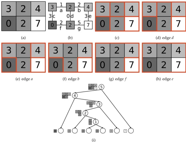
(26) 2.2 – Component Trees as Stackable Hierarchies of Regions. 17. 2.2 Component Trees as Stackable Hierarchies of Regions After defining graphs associated to the image domain, subgraphs, image regions, and trees, we propose to formalize the hierarchical structure behind the concept of component tree as a stackable hierarchy of regions (SHoR). Every such hierarchy is based on, or “seeded” in a stack of image region seeds S . S is a. finite sequence of (sub-)graphs defined on a graph G = (V, E) corresponding to an image I with the following properties:. S = (X0 = (V0 , E0 ), . . . , Xl = (Vl , El )),. (2.17). such that ∀i ≥ 1, Ei−1 ⊆ Ei , Vi−1 ⊆ Vi ,. and Vl = V.. Additionally, every subgraph Xi is such that it can be decomposed into one or more connected subgraphs of the image:. ∀i, Xi = (Vi,0 ∪ . . . ∪ Vi,k , Ei,0 ∪ . . . ∪ Ei,k ), k ≥ 0,. (2.18). where each connected subgraph Xi,j = (Vi,j , Ei,j ) defines a connected region Ri,j = ̺(Xi,j ) = ̺(Vi,j , Ei,j ).. A stackable hierarchy of regions (SHoR) HS is then constructed from the stack of image re-. gion seeds S by closing all the different connected subgraphs Xi,j appearing in S in Eq. (2.17). and (2.18). HS is the set of all the connected components Ri,j = ̺(Xi,j ).. An equivalent definition of a stackable hierarchy HS of regions can also be written as:. i) G ∈ HS , ii) for each two elements R1 , R2 ∈ HS the following holds: R1 ∩ R2 6= 0 ⇒ R1 ⊆ R2 or. R2 ⊆ R1 .. An example of SHoR is shown in Fig. 2.1(a), with the subgraphs Xi of the corresponding. stack of image region seeds displayed in Figs. 2.1(b) – 2.1(e).. The most straightforward way to represent inclusion relations between regions in such a hierarchy is by trees, where every node corresponds to a connected region of the image represented by the hierarchy. The regions in the leaf nodes correspond to small image details, coarse structures can be found in the nodes closer to the root, while the root of the tree corresponds to the whole image domain. Parental relations between nodes represent inclusion. Image indexing with component trees Petra Bosilj 2016.

(27) Chapter 2 – Formalization of Component Trees. 18. R00. R10. R11 R01. (a) S = (X0 , X1 , X2 , X3 ). (b) X0 = (V00 ∪ V01 , E00 ∪ E01 ). (c) X1 = (V10 ∪ V11 , E10 ∪ E11 ). R30 R20 R20. R21. R30 = I. R10. R11. R00. R01. R21. (d) X2 = (V20 ∪ V21 , E20 ∪ E21 ). (e) X0 = (V30 = V, E30 ). (f) component tree based on S. Figure 2.1: A full example of the SHoR and the stack of image region seeds is shown in subfigure (a). The color orange corresponds to nodes and edges constituting X0 , purple for X1 ,. yellow for X2 and green for X3 . Subfigures (b) through (e) show the sub-graphs that are the building parts of S . In the representation of every subgraph, Xi , the grayed out nodes and. edges, as well as black edges, are not part of the subgraph Xi . Connected regions based on connected subgraphs of different Xi are encircled, and marked in the images. The stackable. hierarchy of regions (SHoR) is finally equal to HS = {R00 , R01 , R10 , R11 , R20 , R21 , R30 = I }. The subfigure (f) displays the component tree corresponding to the SHoR in subfigure (a),. where the colors used to enclose the connected regions Ri,j are utilized in the tree as the colors of the corresponding nodes.. relation between the regions, i.e. the set of pixels of the child region is a subset of the set of pixels of its parent (and all his ancestors). A simple example of such a tree, based on the SHoR from Fig. 2.1(a), is shown in Fig. 2.1(f). To formalize the tree structure as a representation of the SHoR, some constraints are imposed on the general definition of the tree following the definition of HS . In a tree T =. ( M, P) which corresponds to a SHoR of an image I (with corresponding G = (V, E)), the. Image indexing with component trees Petra Bosilj 2016.

(28) 2.3 – Categorization of Tree Representations into Superclasses. 19. region represented by a node n ∈ M is denoted by R(n) = (V (n), E(n)). The root node of. the tree T , r ∈ M such that ID(r) = 0 corresponds to a region covering the whole image, i.e.. R(r) = G = (V, E). For any two nodes, n and m it is either true that their sets of pixels are disjoint, V (n) ∩ V (m) = ∅, or one of the following holds: V (m) ⊆ V (n) or V (n) ⊆ V (m). If V (m) ⊆ V (n), we say that n is an ancestor of m, i.e. n is one of the nodes on the path P from the root r to m. The relation between the region represented by a parent node and the regions represented by its children can be formalized as follows. If m is a parent node in the tree and n1 , . . . , nk are all the children of m, the following rules describe how to construct m from its children: V ( m ) = V ( n1 ) ∪ . . . ∪ V ( n k ) ∪ S ( m ),. (2.19). where S ( m ) = { p0 , . . . , p l }, l ≥ 0. (2.20). such that ∀i ∈ {0, . . . , l }, pi ∈ I. ∀ j ∈ {1, . . . , k}, pi 6∈ V (n j ).. The edge set of the parent can be represented as: E(m) = {e p,q ∈ E| p ∈ V (m), q ∈ V (m)},. (2.21). and the pixel set S(m) has to be such that the following holds:. R(m) = (V (m), E(m)) is a connected region of I.. (2.22). The equation (2.19) dictates that a pixel set of the parent can be written as a union of the pixel sets of all its children, and optionally some additional pixels. The set of additional pixels S(m) in Eq. (2.20) can be empty, allowing for the parent region to consist only of its (adjacent) children regions, but also allows us to construct a parent from non-adjacent regions by including new pixels using the set S(m) so that the newly constructed region is still connected according to Eq. (2.22). The equation (2.21) only ensures that the newly constructed subgraph R(m) is indeed a region with the vertex set V (m).. 2.3 Categorization of Tree Representations into Superclasses Equations (2.19)–(2.22) are general relations describing all types of trees. In this subsection, we present a categorization of all the tree classes into two superclasses and further constraints to the equations in order to specialize them for each of the superclasses. Such a categorization was already proposed in [30], and is explored here in more detail with added. Image indexing with component trees Petra Bosilj 2016.

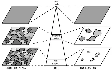
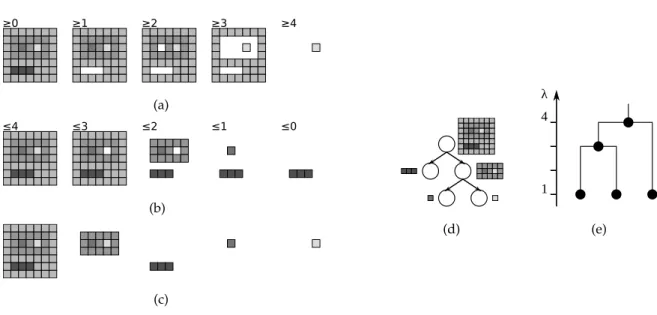
(29) Chapter 2 – Formalization of Component Trees. 20. illustrations and explanations. Based on the properties of the nodes and the nature of parentchild relations in the tree representations, we can distinguish between two different superclasses: • Inclusion trees: the leaves contain only the finest image structures (typically, local. extrema of pixel gray levels) and do not form a complete partition. Inner nodes are formed by region growing from the leaves until there is only one region (the root of the tree) covering the entire image domain.. • Partitioning trees: all the nodes of any cut of the tree form a full partition of the image.. The initial partition contained in the leaves is a fine image segmentation. A parent node is an union of all its children with no additional pixels.. Such a categorization corresponds well to partitions and partial partitions: the stack of image region seeds S used in the construction of a partitioning tree will always comprise. subgraphs that are partition of the image, while the set S of an inclusion tree will comprise partial partitions.. Inclusion trees. The leaf nodes of inclusion trees do not cover the whole image domain. Instead, they hold isolated points or small regions, typically local maxima or minima [88, 159] of the image, or both [120]. This way, the nodes in (and close to) the leaves correspond to bright or dark details of the image. As already mentioned, the stack of image region seeds. S used in construction of an inclusion tree comprises partial partitions. The support of these partial partitions is nested, that is, the relations in Eq. (2.17) hold for any supp(Xi−1 ) and supp(Xi ) as well. Additionally, any cut of an inclusion tree is a partial partition as well. New nodes are formed by a region growing process starting from the leaves, by adding one or more pixels (usually the whole image flat zones) to the regions in the leaf nodes. When the regions of two or more nodes merge in the course of this process, the newly constructed node becomes a parent of all the nodes representing the merged regions thus unifying several tree branches. This process continues until there is only one region covering the whole image domain, and the node representing this region becomes the root of the constructed hierarchical representation. In order to reflect the structure of inclusion trees, we add a further constraint in Eq. (2.19)–(2.22). The only modification is adding a strict inequality in Eq. (2.20), l > 0, to reflect that regions are only formed by adding new pixels to already existing regions (or a single region). Simplifying the image represented by an inclusion tree includes cutting (removing) some branches from the leaves to the desired point (usually, up to a region satisfying a certain criterion). The areas of the removed regions are then assigned a gray level of the closest surviving ancestor node (i.e. the ancestor node with the greatest distance from the root) of. Image indexing with component trees Petra Bosilj 2016.

(30) 2.4 – Indexing the SHoR. 21. the regions that were cut off. This accomplishes removing small dark or bright structures in the image without changing the larger structures. Partitioning trees. The principal difference of partitioning trees when compared to inclusion trees is that the leaves of the structure always form a (very fine) image partition. The same is true for any cut of such a tree [76] (as well as all the subgraphs Xl from the stack of image seeds S used in construction). The initial partition contained in the leaves can be the result of any segmentation algorithm, but among most common choices are the image pixels, flat-zones of the image [202, 173] or the result of watershed segmentation [100]. Regions of the inner nodes of the trees are formed by merging, as unions of the adjacent regions of other nodes, meaning that every new node has at least two child nodes. In contrast to the leaf nodes, a cut higher in the tree is a coarser segmentation of the image. To formalize this, a constraint k > 1 has to be added to Eq. (2.19) and l = 0 to Eq. (2.20) to reflect that no pixels are added that did not previously belong to a node. Notions needed to define the iterative merging, which is at the core of the construction process of any partitioning tree were first introduced by Garrido et al. [72] (and only later put in the context of trees [158]): 1. Region model defines how simple regions and their unions are represented. It reflects the characteristics of the regions used in the construction process. 2. Merging criterion or similarity (or dissimilarity) measure describes the interest of possible merges. It is based on the region characteristics represented by the region model. 3. Merging order defines the rules used to merge the regions and which merge to perform next based on the merging criterion. In order to simplify an image using a corresponding partitioning tree, a coarse enough cut is selected in the tree (the decision can be based e.g. on the number of desired elements of the partition or some more complex criteria). Each region represented by a node in the cut is then represented by a uniform gray level, which can be based on the region model, or take into account the average gray level of the region. This way, small variations in the gray levels of image pixels of can be removed from regions perceived as uniform. The difference between inclusion and partitioning trees is shown in Fig. 2.2.. 2.4 Indexing the SHoR While trees are sufficient to represent the inclusion relations between the regions in a SHoR, it is often desirable to assign an attribute to each node, corresponding to a measure of aggregation, called the level (of aggregation) of the node. Such an attribute λ is a non-negative. Image indexing with component trees Petra Bosilj 2016.

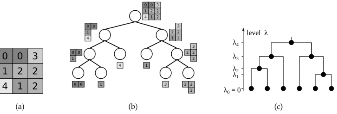
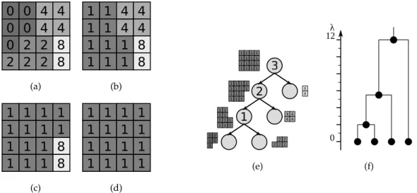
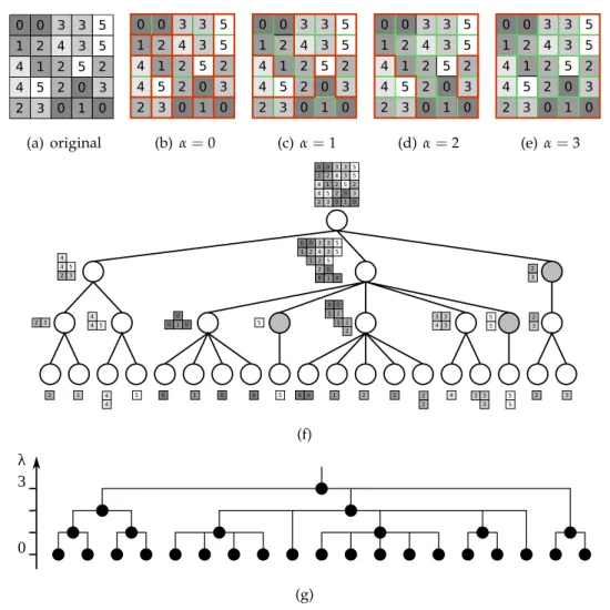
(31) Chapter 2 – Formalization of Component Trees. 22. root node. middle nodes. leaf nodes. PARTITIONING. TREE. INCLUSION. Figure 2.2: This image demonstrates the difference between the superclasses of partitioning and inclusion trees. Cuts of the partitioning tree near its bottom and the middle, as well as the root node are displayed on the left. A set of nodes from the inclusion tree close to the bottom and middle of the tree, and the root of the tree are displayed on the right. function of the nodes. A tree with levels assigned in such a manner is then considered indexed. The attribute values λ are usually determined based on the definition or the construction algorithm for a specific tree. The rule for assigning the levels always reflects the fact that the coarseness of the nodes increases along each branch from the leaves towards the root and states that if m is an ancestor of n, then λ(n) < λ(m). Hereafter, we explain the wellestablished representational framework for indexed partitioning trees [87, 83, 135]. We furthermore propose the way to represent the indexed inclusion trees in the same framework, whereas there is no current convention about the representational framework for inclusion trees. An ultrametric distance is a constraint stronger than a distance on a set of elements, where the elements of the set obey an inequality stronger than the triangular inequality: the ultrametric inequality. An ultrametric inequality states that for any three elements of a set, v1 , v2 , v3 ∈ Ω, it is true that d(v1 , v2 ) ≤ max(d(v1 , v3 ), d(v2 , v3 )). If, while indexing a par-. titioning tree, we add an additional constraint λ(n) = 0 if and only if n is a leaf node, then there is a bijection between indexed partitioning trees and ultrametric distances [87, 83] defined on a same set. The definitions and construction algorithms of different types of partitioning trees always assign the same attribute value (usually λ = 0) to all the leaf nodes, so this additional constraint is in accordance with how the attribute value is naturally assigned for the partitioning trees. The levels of such an indexed partitioning tree induce an ultrametric distance on the nodes of the tree and the pixels of the image. To all the vertices of an image graph G = (V, E), with a corresponding SHoR and partitioning tree T , we can assign the. Image indexing with component trees Petra Bosilj 2016.

(32) 2.4 – Indexing the SHoR. 23 0 0 3 1 2 2 4 1 2 3. 0 0 1. 2 2. 4. 1 2. level λ 3. 0 0 3. 2 2. 0 0. 2. 1 4. 1. 0 0. 1. 3. 2 2 2. (a). λ3 λ2 λ1. 1 2 2 4 1 2. λ4. λ0 = 0. (b). (c). Figure 2.3: Subfigure (b) shows a possible partitioning tree constructed for the image shown in subfigure (a). A dendrogram, corresponding to one possible indexing of the tree, is displayed in (c). following ultrametric distance: d(v1 , v2 ) = min{λ(n)|n ∈ T , v1 ∈ V (n), v2 ∈ V (n)}. (2.23). According to Eq. (2.23), a distance between any two image elements from I is given by the smallest level of a node n representing a region containing both image elements. Such indexed trees are conveniently represented in a form of a dendrogram [179], first introduced under the name taxonomic tree [172] for the purpose of hierarchical clustering. The height of each node in a dendrogram corresponds to the level assigned to that node (cf. Fig. 2.3). The reasoning behind using a separate representation for the structure of the hierarchy and to display the indexing imposed upon a hierarchy is that only the structure (in terms of inclusion relations) does not include all the information provided by the tree construction process. While comparing the tree structures would allow one to compare the composition of the image in terms of object and region inclusion, the indexing is usually needed when reconstructing the image and in other tasks where contrast between the regions (or other information used to construct the tree) is important. In order to represent the inclusion trees in a similar manner, we propose extending them so their leaves partition the image. This corresponds to adding new child nodes to cover the regions previously added to the hierarchy through the non-empty sets S(n) for every parent node n. Another issue is that the definitions and construction algorithms of inclusion trees often dictate assigning attribute values different from 0 and different from each other to the leaf nodes of the original tree (as will be detailed in Sec. 3). To resolve this in a uniform way, we will be adding new nodes as the children of all the original leaf nodes. As the extended tree is a partitioning tree, is it necessary to avoid having a node with a single child. For this reason, we will always be extending the tree with pairs of nodes.. Image indexing with component trees Petra Bosilj 2016.

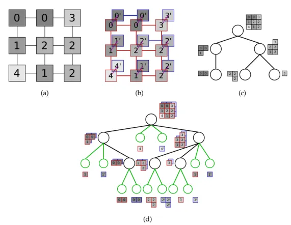
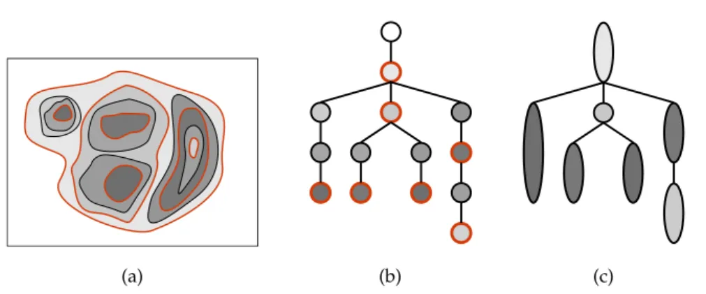
(33) Chapter 2 – Formalization of Component Trees. 24. 0 1 4. 0 2 1. 0'. 3. 0. 0'. 1'. 2. 1. 4. 2'. 1 2 2 4 1 2. 2'. 3. 2 1'. 0 0. 2 2. 1. 1 2. 2'. 1. (a). 0 0 3. 3. 2 4'. 2. 3'. 0. 0 0. 2. 3. 2 2 2. (b). (c) 00' 00' 33' 11' 22' 22' 44' 11' 22'. 33' 22' 22' 1' 1 22'. 00' 00' 11' 4. 00' 00'. 1. 4'. 33'. 22' 22' 22'. 1. 1'. 0 0. 0' 0'. 2 2. 2' 2'. 2. 2'. 3. 1'. 3'. (d). Figure 2.4: A possible inclusion tree for the image displayed in subfigure 2.4(a) is shown in subfigure 2.4(c). The extended image which includes the ghost regions is shown in subfigure 2.4(b), where the links between original image pixels are shown in red. The pixels of the ghost regions only have the connections to the ghost pixels belonging to the same ghost region, and are displayed in blue. Every ghost pixel is also connected to the corresponding pixel of the original image (purple links). The extended tree is shown in the subfigure 2.4(d) with the auxiliary nodes shown in green. The doubling of the represented regions for the inner nodes is due to the fact that they include both the original flat zones as well as their ghost region pairs. All the nodes added by such an extension will be leaves of the extended tree, and will be considered auxiliary nodes. When extending the tree with the auxiliary nodes, we have to do it in a way that enables differentiating the auxiliary nodes from all the nodes present in the original tree. Henceforth, we explain our proposition for extending the tree in a way that can be indexed and represented by a (reduced) dendrogram. First, we extend the original image with ghost regions corresponding to every flat zone (cf. the original image on Fig. 2.4(a) and extended image on Fig. 2.4(b)). For every flat zone. Fk at every intensity level k in the image, a ghost region Fk′ is considered to be connected to Fk . A pair of auxiliary nodes holding the original flat zone region Fk and the corresponding ghost region Fk′ are added to the tree. The parent of this new pair of auxiliary nodes is the. Image indexing with component trees Petra Bosilj 2016.

(34) 2.4 – Indexing the SHoR. 25 level λ. level λ λ4. λ4. λ3. λ3. λ2. λ2. λ1. λ1. λ0 = 0. λ0 = 0. (a). (b). Figure 2.5: Subfigure (a) shows a dendrogram representation of a possible indexing of the extended tree displayed in Fig. 2.4(d). The reduced dendrogram corresponding to the same indexing is shown in subfigure (b). The only nodes displayed in the reduced dendrogram are the nodes of the original inclusion hierarchy, displayed in Fig. 2.4(c). first node in the tree containing pixels of Fk . In the extended tree, all the original nodes of the. inclusion tree include all of their original flat zones, as well as all the corresponding ghost regions. The original tree, corresponding to the image in Fig. 2.4(a), is shown in Fig. 2.4(c). After extending the image with ghost regions, as in Fig. 2.4(b), the extended tree corresponding to this extended image is shown in Fig. 2.4(d). In the tree extended in this way, the leaf nodes of the original inclusion tree can be identified as the only nodes having only the (new) leaf nodes as children. Any other node n of the extended tree that has leaf nodes as children has had a non-empty set S(n) in the original tree. All the auxiliary nodes, that is the nodes representing the flat zones and their ghost regions, are assigned the level 0, λ(Fk ) = λ(Fk′ ) = 0, ∀Fk , Fk′ . In order to ensure λ(n) > 0 for. all other nodes of the tree, we add a constant value to the attribute assigned to every node by the construction algorithm or based on the tree definition. For reasons of simplicity, in most examples, this constant will be equal to 1. With this kind of extension, the Eq. (2.23) holds for indexed extended inclusion hierarchies as well. The inclusion tree extended in this manner can be directly represented by a dendrogram, and a dendrogram corresponding to the possible indexing of the extended tree of Fig. 2.4(d) is displayed in Fig. 2.5(a). However, since the auxiliary nodes are usually not in the focus of the representation, we propose to represent the inclusion trees by reduced dendrograms. All the auxiliary nodes have the attribute λ(n) = 0, and are the only nodes with this attribute value (a constant is added to attributes of all other nodes). Thus, we propose to simply omit them from the representation. In the resulting reduced dendrogram, the auxiliary nodes are still considered to be present, but are hidden and not displayed. An example of a reduced dendrogram indexing the tree in Fig. 2.4(c), and corresponding to the same possible indexing as the full dendrogram in Fig. 2.5(a), is shown in Fig. 2.5(b).. Image indexing with component trees Petra Bosilj 2016.

(35) Chapter 2 – Formalization of Component Trees. 26. When indexing the inclusion tree, we encounter the same problem as Ronse when trying to represent an output of a segmentation algorithm producing a residual in the framework of connective segmentations and partitions. Directly adding the residual to the representation (or in our case, the nodes covering the regions of non-empty sets S(n)) to cover the whole image domain makes them indistinguishable from the original leaf nodes. However, while Ronse constricted the domain of the partition to the support [155], we instead chose to extend the domain. Constricting the domain in an (inclusion) hierarchy is difficult as the support changes through the hierarchy (cf. Subsec. 2.3, the supports are nested). By instead doubling the domain, we can extend an inclusion to a partitioning hierarchy (on an unchanging domain), and index it.. Chapter Summary In this chapter, the basic notions used herein are first introduced. In addition to traditional formalization of hierarchical image representations, we offer a new formalization through stackable hierarchy of region (SHoR). Based on this formalization, we propose a classification of trees into two superclasses, namely inclusion and partitioning tree. Finally, indexing is introduced as a way to assign a level of aggregation to the elements of the hierarchy, imposing an ultrametric distance on the elements of the hierarchy. We extend the existing indexing principles as well as a representation and visualization framework using dendrograms used to handle partitioning trees, and apply them to inclusion hierarchies as well. In the next chapter, we present different examples of both partitioning as well as inclusion hierarchies. An indexing method (i.e. a way to assign levels to the hierarchy) reflecting the construction process of each examined tree is proposed. Each inclusion tree is represented by its reduced dendrogram, and each partitioning tree by its dendrogram.. Image indexing with component trees Petra Bosilj 2016.

(36) 27. Chapter. 3. Overview of Component Trees. Contents 3.1. Min and Max-trees . . . . . . . . . . . . . . . . . . . . . . . . . . . . . . . . .. 28. 3.2. Tree of Shapes . . . . . . . . . . . . . . . . . . . . . . . . . . . . . . . . . . . .. 32. 3.3. Binary Partition Tree . . . . . . . . . . . . . . . . . . . . . . . . . . . . . . . .. 36. 3.4. α-tree . . . . . . . . . . . . . . . . . . . . . . . . . . . . . . . . . . . . . . . . .. 45. 3.5. (ω )-tree . . . . . . . . . . . . . . . . . . . . . . . . . . . . . . . . . . . . . . .. 48. 3.6. Comparative summary . . . . . . . . . . . . . . . . . . . . . . . . . . . . . . .. 51. This chapter presents the details and characteristics of a large number of hierarchical image representations, based on the comprehensive study by the author [29]. Their structure is presented withing the context of a taxonomy based on simplifications in the definition of the hierarchies applicable to a large number of tree representations. Indexing the hierarchies is done in an established framework based on dendrograms, presented and extended in Chap. 2 to enable indexing the full range of presented hierarchies. This comprehensive presentation of the trees and their characteristics was complemented by a summary of construction algorithms used to implement the hierarchies. The interest in such hierarchies is validated by the recent increase in processing techniques interacting with image regions or superpixels rather than individual image elements and requiring a representation extending through multiple scales, as well as a wide range of application domains attempting approaches based on trees specifically.. Image indexing with component trees Petra Bosilj 2016.

(37) Chapter 3 – Overview of Component Trees. 28. Table 3.1: Classification of the presented trees. tree inclusion. Min and Max-tree (Sec. 3.1) Tree of Shapes (Sec. 3.2). partitioning. Binary Partition Tree (Sec. 3.3). Topological ToS (Subsec. 3.2.1) BPT by Altitude Ordering (Subsec. 3.3.1) Hierarchies of MSF (Subsec. 3.3.2). α-tree (Sec. 3.4). (ω )-tree (Sec. 3.5) The characteristics of 5 distinct hierarchical representations, as well as 3 different special cases of those hierarchies are analyzed in detail and compared. In addition to explaining the structure of each hierarchy, they are mutually compared based on their characteristics of duality, ability to represent objects, completeness of the representation and complexity of construction. Additionally, the possibility of adapting the different representations using parametrization, where applicable, is also explored. The high-level, detailed study of the tree characteristics presented here offers a way to compare the presented representations independently of the intended application as well as it offers an extensive number of references concerning the recent advances as well as seminal historical work pertaining to the representations. The characteristics the trees exhibit are examined and summarized for every introduced tree, as well as compared to characteristics of other presented trees. First, the trees from the inclusion tree superclass are listed, followed by partitioning trees. Following the definition of each tree, the most efficient algorithms suited for their implementation are discussed. The summary of different trees and their sub-types according to this classification is shown in Tab. 3.1. The chapter concludes by considering and comparing all the characteristics of all the trees considered in Subsec. 3.6. 3.1 Min and Max-trees Min-trees (and their dual structure, Max-trees) are from the superclass of inclusion trees. The concept and examples will first be given for the Min-tree structure, with the duality between trees explained at the end of the section. The Min-tree is a structure aimed at representing the dark structures of the images. The. Image indexing with component trees Petra Bosilj 2016.

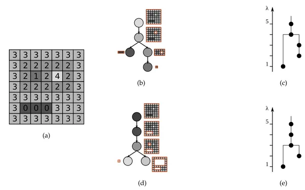
(38) 3.1 – Min and Max-trees. 29 λ 5. 3 3 3 3 3 3 3. 3 2 2 2 3 0 3. 3 2 1 2 3 0 3. 3 2 2 2 3 0 3. 3 2 4 2 3 3 3. 3 2 2 2 3 3 3. 3 3 3 3 3 3 3. 1. (b). (c). λ 5. (a). 1. (d). (e). Figure 3.1: The original image is displayed in subfigure (a). Subfigure (b) shows the corresponding Min-tree, with the reduced dendrogram shown in (c). The Max-tree and its reduced dendrogram for the same image are shown in subfigures (d) and (e). Regions corresponding to the nodes in both subfigures (b) and (d) are shown next to the nodes (the white parts do not belong to the regions). leaves of the image represent the regions corresponding to local minima in the image. All inner nodes are connected components of lower level sets of the image. A connected component of the level set Lk will make a new node nk with a region R(nk ).. This node can either become:. • a parent node to all the previously constructed nodes at lower levels which are included in the region of the new node: R(nk′ ) ⊂ R(nk ), k′ < k,. • a leaf node if it does not include the regions of any previously constructed nodes. Finally, the level set LlMax at the highest gray level present in the image (usually lMax = 255). has only one connected component covering the whole image domain. This becomes the root of the tree, unifying all branches of the tree. An example of the Min-tree can be seen in Fig. 3.1(b). This structure is not self dual: trying to construct a Min-tree of the dual image − I will. produce a different output since the local minima in the original image correspond to the local maxima of the dual. The dual structure of the Min-tree is the Max-tree: it can be seen as. Image indexing with component trees Petra Bosilj 2016.