UNIVERSITÉ DU QUÉBEC À MONTRÉAL
MODELLING OF THERMAL CONVECTION
IN THE EARTH'S MANTLE
THESIS SUBMITTED AS PARTIAL REQUIREMENT FOR
THE DEGREE OF DOCTOR OF PHILOSOPHY
IN EARTH AND ATMOSPHERIC SCIENCES
BY
PETAR GLISOVIé
Service des bibliothèques .
Avertissement
La diffusion de cette thèse se fait dans le respect des droits de son auteur, qui a signé le formulaire Autorisation de reproduire et de diffuser un travail de recherche de cycles supérieurs (SDU-522 - Rév.01-2006). Cette autorisation stipule que «conformément
à
l'article 11 du Règlement no 8 des études de cycles supérieurs, [l'auteur] concèdeà
l'Université du Québecà
Montréal une licence non exclusive d'utilisation et de publication de la totalité ou d'une partie importante de [son] travail de recherche pour des fins pédagogiques et non commerciales. Plus précisément, [l'auteur] autorise l'Université du Québec à Montréal à reproduire, diffuser, prêter, distribuer ou vendre des copies de [son] travail de rechercheà
des f.ins non commerciales sur quelque support que ce soit, y compris l'Internet. Cette licence et cette autorisation n'entraînent pas une renonciation de [la] part [de l'auteur]à
[ses] droits moraux nià
[ses] droits de propriété intellectuelle. Sauf entente contraire, [l'auteur] conseNe la liberté de diffuser et de commercialiser ou non ce travail dont [il] possède un exemplaire.» ·UNIVERSITÉ DU QUÉBEC À MONTRÉAL
MODÉLISATION DE LA CONVECTION THERMIQUE
DANS LE MANTEAU TERRESTRE
THÈSE PRÉSENTÉE
COMME EXIGENCE PARTIELLE DU
DOCTORAT EN SCIENCES DE LA TERRE ET DE L'ATMOSPHÈRE
PAR
PETAR GLISOVIé
This thesis would not have been possible without the guidance, encouragement and generous financial support of my mentor, Professor Alessandro Forte. His fatherly ad vice and friendship has been invaluable on both an academie and a personallevel, for which 1 am extremely grateful. 1 would like to thank Professors Jean-Claude Mareschal and Fiona Darbyshire for the ir help, and kindness, teaching me important !essons on both geophysics and humanity over the past four years. Also, 1 would like to thank Professor Jerry X. Mitrovica for valuable suggestions and comments that improve the final version ofthesis.
I enjoyed many inspirational discussions with Professor Robert Moucha, and Xavier Robert. To Professor Moucha, 1 owe special thanks for his great patience, and for his kindly guidance that have lead me through this exciting and difficultjourney. A Iso, 1 am very grateful to my dear friend Paul Auerbach for promoting a stimulating and welcoming social environment tome and my family.
The simulations used in this study are computed on the supercomputing facilities of the SciNet consortium at the University of Toronto. 1 thank the stuff of the SciNet for their support. My special thanks to my parents, sister, and brother for the ir selfless love, and unconditional support.
Finally, I owe my deepest gratitude to my wife Sanja and my son Andrej for the ir understat-ing, and whose unlimited love has been my deep weil of strength during ail these years.
TABLE OF CONTENTS LIST OF FIGURES 0 0 0 0 0 0 0 0 0 0 0 0 0 0 o 0 0 0 0 0 0 0 0 0 0 0 0 0 0 0 0 0 0 0 0 0 0 0 0 0 vt LIST OF TABLES 0 0 0 0 0 0 0 0 0 0 0 0 0 0 0 0 0 0 0 0 0 0 0 0 0 0 0 0 0 0 0 0 0 0 0 0 0 0 0 0 0 xv RÉSUMÉ 0 0 XV li ABSTRACT 0 0 0 0 0 0 0 0 0 0 0 0 0 0 0 0 0 0 0 0 0 0 0 0 0 0 0 0 0 0 0 0 0 0 0 0 0 0 0 0 0 0 0 0 XIX fNTRODUCTION 0 0 0 0 0 0 0 0 0 0 0 0 0 0 0 0 0 0 0 0 0 0 0 0 0 0 0 0 0 0 0 0 0 0 0 0 0 0 0 0 0 CHAPTERI
TIME-DEPENDENT CONVECTION MODELS OF MANTLE THERMAL STRUC-TURE CONSTRAINED BY SEISMIC TOMOGRAPHY AND GEODYNAMICS: IM-PLICATIONS FOR MANTLE PLUME DYNAMICS AND CMB HEAT FLUX 0 0 0 0 0 5
1.1 Résumé 0 0 0 0 0 0 0 0 0 0 0 0 0 5
102 Abstract 0 0 . 0 0 0 0 0 0 0 0 0 7
1.3 Introduction 0 0 0 0 0 0 0 0 0 0 9
1.4 Numerica1 Method 0 0 0 0 0 0 12
1.401 Equations for thermal convection in an anelastic, compressible, self-gravitating mantle 0 0 0 0 0 0 0 0 0 0 0 0 0 0 0 0 0 0 0 0 0 0 0 0 0 0 0 0 0 0 0 0 0 0 0 0 0 0 0 0 12 1.402 A spectral solution of the gravitationally consistent equations of mass and
momentum conservation 0 0 0 0 0 0 0 0 0 0 0 0 0 0 17 1.403 Solving the equation of conservation of energy 0 0 0 0 0 0 0 0 0 24 1.4.301 Pseudo-spectral method 0 0 0 0 0 0 0 0 0 0 0 0 0 0 0 . 0o 0 0 0 0 0 0 0 24
1.4.3.2 Time-integration oftemperature . . . . 26 1.4.4 Determination of a geotherm -the energy balance criterion . 27 1.5 Initial conditions and reference properties of the mantle 27 1.6 Results . . . . 30 1.6.1 Numerical issues in the upper part of the mantle 30
1.6.2 Steady-state geotherm and energy balance 33
1.6.3 Lateral heterogeneity and flow patterns 36
1.7 Discussion .. . .. .. . . .. .. . 39
1.A Pseudo-Spectral Numerical Solution ofthe Energy Conservation Equation 46
1.A.1 Diffusion operator . . 46
l.A.2 Advection . . . .
48
1.A.3 Dissipation and internai heating 49
1.A.4 Solution of the equation of energy conservation 50
l.A.4.1 Numerical scheme . . . . .. . 50
l.A.4.2 Thermal boundary conditions . 52
l.A.4.3 Solution of the system . . . 53
1.A.4.4 Numerical stability requirements . 54
l.A.4.5 Alias-free transformations. 54
1.8 Computational aspects ofthe numerical code 55
CHAPTERII
IMPORTANCE OF INITIAL BUOYANCY FIELD ON EVOLUTION OF MANTLE THERMAL STRUCTURE: IMPLICATIONS OF SURFACE BOUNDARY CONDITIONS 74
2.1 Résumé . 74
2.2 Abstract 75
2.4 Numerical madel, initial conditions and reference frame . 2.4.1 Initial geotherm . . . .
2.4.2 Initial mantle heterogeneity . 2.4.3 Surface boundary conditions 2.4.4 Reference state of the mantle . 2.5 Results and discussion
2.5.1 Rigid surface .
2.5.2 Surface with tectonic plates coupled to the mantle flow .
2.6 Conclusions . . . .. .. .. . . .. . .. . . .
CHAPTERIII
TIME-REVERSED MANTLE CONVECTION BASED ON THE 3-D TOMOGRAPHie IMAGES: QUANTIFYING ROBUSTNESS OF THE QRV AND BAD MO DELS OVER
IV 76 77 77 78 79 80 80 83 86
THE CENOZOIC ERA . 99
3.1 Résumé . 99
3.2 Abstract 100
3.3 Introduction . 101
3.4 Numerical Method 104
3.5 Description ofModels 106
3.5.1 Reference Properties ofthe Mantle 106
3.5.2 Initial Conditions 106
3.6 Results . . . 109
3.6.1 Reconstruction of Steady-State Solution over 65 Myr Interval 109
3.6.2 Reconstruction of Cenozoic Era 112
3.7 Discussion . . . 115
308 Solution of the regularized equation of energy conservation 30801 Numerical scheme 0 0 0 0 0 0 0
3oBo2 Thermal boundary conditions 0 30B03 Solution of the system 0 0 0 0 0 30B.4 Numerical stability requirements 0
119 119 121 122 123 CONCLUSION 0 0 0 0 0 0 0 0 0 0 0 0 0 0 0 0 0 o 0 0 0 0 0 0 0 0 0 0 0 0 0 0 0 0 0 0 0 0 0 0 0 0 139 8IBLIOGRAPHY 0 0 0 o 0 0 0 0 0 0 0 0 0 0 0 0 0 0 0 0 0 0 0 0 0 0 0 0 0 0 0 0 0 0 0 0 0 0 0 0 0 145
LIST OF FIGURES
FIGURE Page
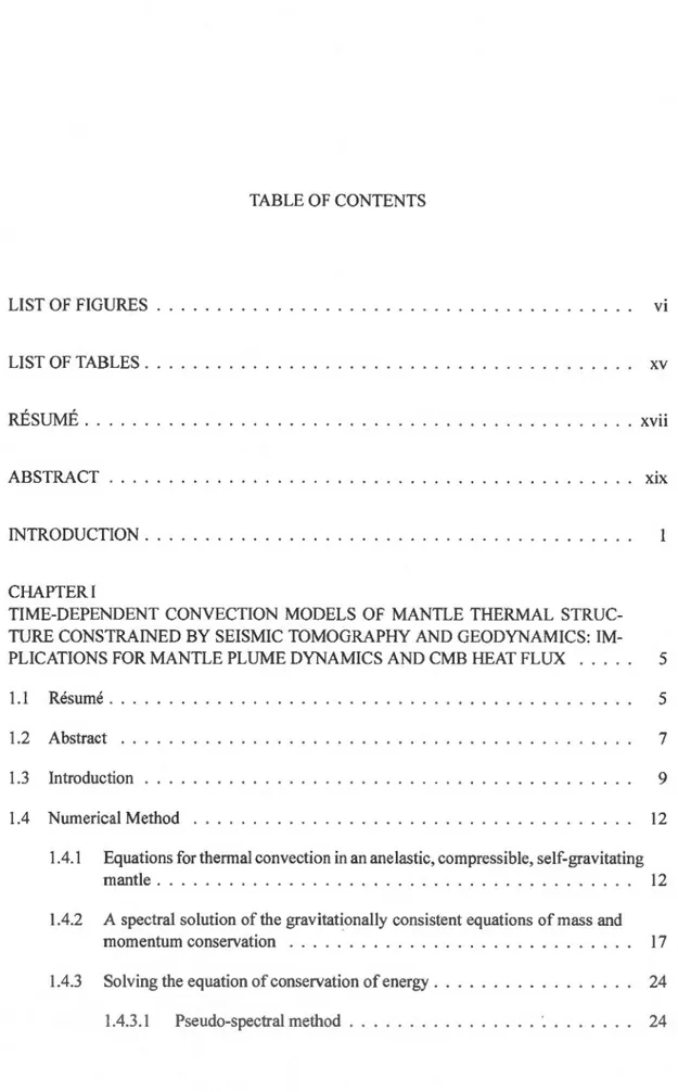
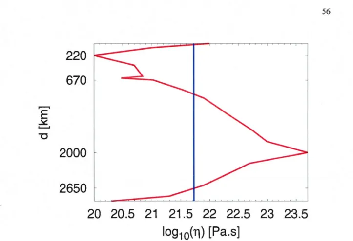
1.1 Viscosity profiles. The geodynamically inferred (Mitrovica & Forte (2004) and Forte et al. (20 1 0)) V2-profile (red 1 ine) is characterized by a two order of mag-nitude reduction in viscosity across the uppermost mantle, where 220 km is the depth at which the V2-profile has minimum viscosity. Deeper in the mantle, there is a great increase in viscosity, about 1600x, from 635 km to 2000 km depth -where the latter corresponds to the depth of maximum viscosity in the mantle. ln the lower 900 km of the mantle, the V2 profile exhibits a 3-order of magnitude decrease of viscosity extending down to the CMB. The ISO V-profile (blue line), is constant and characterises a logarithmic average of the whole-mantle value derived from the V2 profile. . . . . . . . . . . . . . 56 1.2 The root-mean-square (rms) spectral amplitudes of the mantle temperature
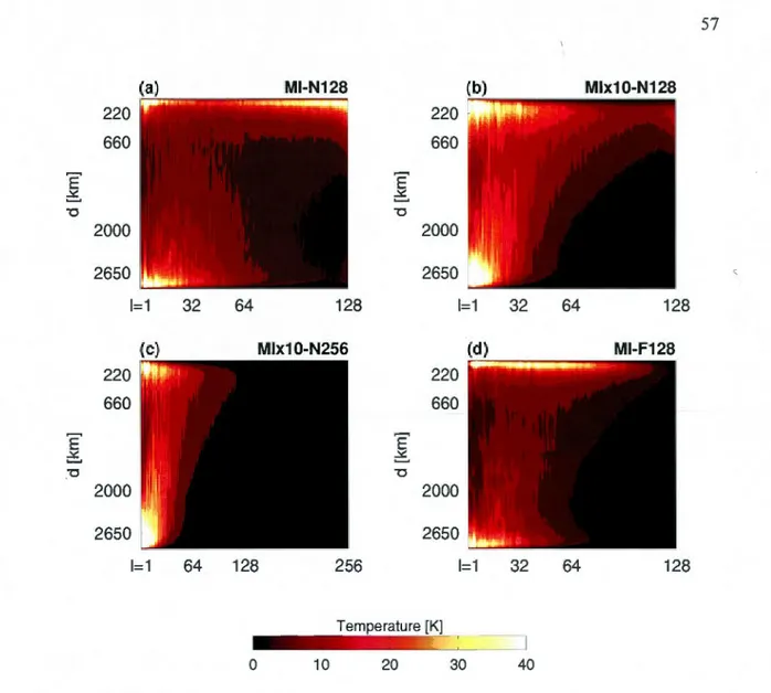
het-erogeneity for iso-viscous convection models after 290 Myr oftime integration from the point of 3.845 Ga (see text). The rms amplitudes are represented on the Kelvin-temperature scale as a function ofspherical harmonie degree (y-axis) and depth (x-axis). . . . . . . . . . . . . . . . . . . . . . . . . 57 1.3 The root-mean-square (rms) spectral amplitudes ofthe mantle temperature
het-erogeneity (y-axis) as a function of spherical harmonie degree (x-axis) for V2 convection models at different depths: (a) 84 km, (b) 224 km after 250 Myr of time integration from the present-day. The blue line indicates the MV2-N256 mode!, and the red line shows the MV2xl O-N256 mode! (see text). . . . . . 58
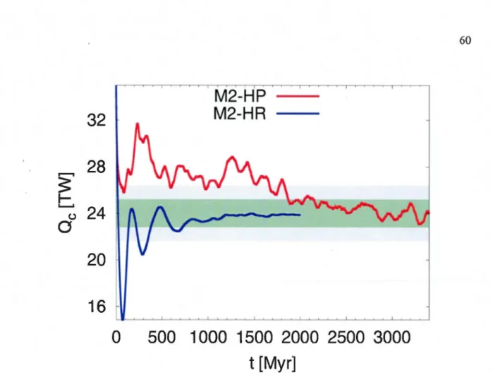
1.4 (a) The root-mean-square (rms) spectral amplitudes of R = 64 (y-axis) as a function ofChebyshev polynomial degree (x-axis) for the iso-viscous MI-NI28 (without filter) mode! at different points of time: 310 Ma (blue li ne), 410 Ma (red line) and 510 Ma (cyan line). (b) The temporal evolution ofthe local rms error of the predictor-corrector time-stepping method for the iso-viscous simu-lations: MI-N128 (blue curve) and MI-F128 (with filter, red curve). The green ( dashed) curve re presents the logarithm ic variations of total integrated kinetic energy for the MI-N128 mode! over 800 Myr. . . . . . . . . . . . . . . . . 59 1.5 Time-dependent internai heating. The temporal evolution of internai heat
pro-duction (Qe) for two convection simulations (M2-HP, with surface plates and M2-HR, with rigid surface) is calculated by differencing the heat flux at the sur-face (F8) and CMB (Fe), such that Qc = F8- Fe. The green rectangle represents a 5% deviation with respect to the expected steady-state value (i.e., 24 TW of imposed internai heating), while the grey represents a 1 0% deviation. . . . . . . 60 1.6 Time-dependent heat flux at the surface and CMB. The top and bottom frames
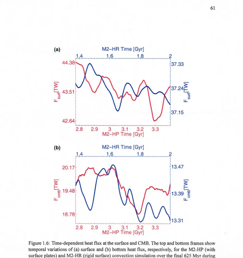
show temporal variations of(a) surface and (b) bottom heat flux, respectively, for the M2-HP (with surface plates) and M2-HR (rigid surface) convection sim-ulation over the final 625 Myr during which steady-state conditions prevail. . . 61 1. 7 Temporal evolution of bulk cooling. The red and blue curves show the
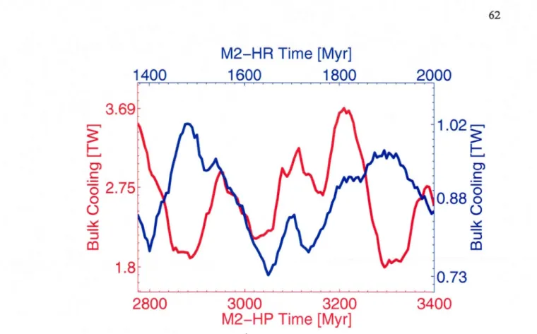
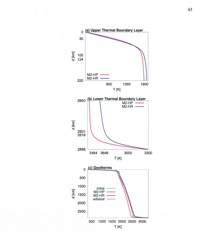
numeri-cally determined bulk cooling of the mantle for the M2-HP (surface plates) and M2-HR (rigid-surface) convection simulations, respectively. These numerically-calculated bulk cooling rates measure the extent to which the mantle geotherm departs from steady-state conditions. . . . . . . . . . . . . . . . . . . . . . . 62 1.8 Global horizontally-averaged mantle thermal structure at the end of the
1.9 Time-dependent evolution of lateral temperature variations driven by mantle convection. In the top two rows are shown equatorial cross-sections of evolving temperature heterogeneity from 65 Ma (left), estimated from seismic tomogra-phy (Simmons et al. (2009)), to 2 Ga into the future (right). The 1 st and 2nd rows show the M2-HP (surface plates) and M2-HR (rigid surface) results, re-spectively. The bottom (3rd) row shows the dominant mode of convection (i.e. maximum spectral amplitude of thermal heterogeneity) as a function of depth at
V Ill
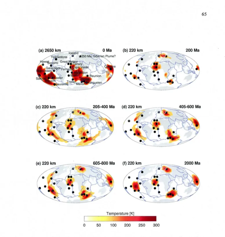
each instant in time. . . . . . . . . . . . . . . . . . . . . . . . . . . 64 1.10 The first map (a) shows the present-day positive heterogeneity (T:?: 100 K) at a
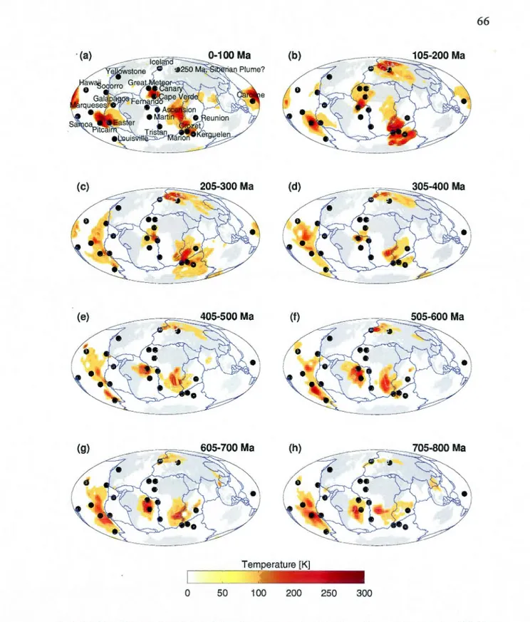
depth of2650 km. The maps from (b) to (f) represent positive lateral temperature variations (T :?: 100 K) at a depth of 220 km obtained by the M2-HR (rigid surface) convection simulations at different points/intervals of time: (b) 200 Ma, (c) 205-400 Ma, (d) 405-600 Ma, (e) 605-800 Ma and (f) 2 Ga. The black circles show the location of present-day hotspots (Courtillot et al. (2003)). . . . 65 1.11 The superimposed 5-Myr time-sequences of positive heterogeneity (T:?: 100 K)
at the depth of220 km obtained by the M2-HP (plates) model at different time-windows (Ma): (a) 0-100, (b) 105-200, (c) 205-300, (d) 305-400, (e) 405-500, (f) 505-600, (g) 605-700 and (h) 705-800. The black circles show the location of present-day hotspots (Courtillot et al. (2003)). . . . . . . . . . . 66 1.12 The temporal variation of total integrated kinetic energy (Ek) in (a) the surface
plates and ( c) rigid-surface convection simulations. It seems that the fluctuations ofkinetic energy (red curve) and the estimated internai heating (Qc, grey curve) are closely coupled. Making a sequence of coupled maximum values for Ek (blue circles) and Qc (green circles) over successive time-windows up to 2 Ga and 1 Ga for the M2-HP and M2-HR models, respectively, we can calculate the difference between the moments of maximum as a function of sequence member -(b)and(d) . . . .. . . .. . . .. . . . 67
1.13 Globally-averaged, root-mean-square (rms) amplitude oflateral temperature vari-ations as a function of depth. The green curve shows the present-day rms tem-perature anomalies derived from seismic tomography (Simmons et al. (2009)). The red and blue curves shows the steady-state temperature anomalies for the M2-HP (surface plates at time 3.4 Ga) and M2-HR (rigid surface at time 2 Ga) convection simulations, respectively. . . . . . . . . . . . . . . . . . . . . . . 68
2.1 The initial horizontally-averaged temperature (i.e., geotherm) and the physical parameters as a function of depth (x-axis) which are used in this study. (a) The initial geotherms taken from a steady-state solution of the thermal convection in the mantle with different surface boundary conditions (Giisovié et al. (20 12)): a rigid surface (blue line) and the dynamically coupled plates (red line). (b) The viscosity profile V2 (Mitrovica & Forte (2004); Forte et al. (2010)). (c) The blue line represents the internai heating due to both the radiative isotopes and the secular cooling, and the red line shows the thermal conductivity profile (Hofmeister (1999)). (d) The density is shown by the blue line, while the red line represents the gravity profile (the PREM mode! ofDziewonski & Anderson (1981)). 0 0 0 0 0 0 0 0 0 0 0 0 0 0 0 0 0 0 0 0 0 0 0 0 0 0 0 0 0 0 0 0 0 0 0 0 0 0 0 0 0 88 2.2 The CMB heat flux (y-axis) as a function of time (x-axis) obtained by: (a) a
rigid surface (R-boundary condition) and (b) the surface tectonic plates coupled to the mantle flow (P-boundary condition). . . . . . . . . . . . . . . . . . 89 2.3 The maps show the lateral temperature variations (in Kelvin) at a depth of 220
km obtained by the IND, EPR, and SAP models with a rigid surface (given by columns) at the different points of time: 350, 1000, and 3000 Ma (given by rows ). The black letter '0' denotes the location of starting mantle heterogeneity, while the steady-state plumes are labelled by numbers (see Table 2.2). . . . 90 2.4 The percentage ratio between the amplitudes ofthe spherical harmonie degree
(x-axis) and the dominant mode of convection as a function of depth (y-axis) for the (a) IND, (b) EPR, and (c) SAP simulations with the rigid surface at 3 Ga. 91
2.5 Map of positive temperature anomaly (red) determined by the present-day seis-mic image (Simmons et al. (2009)) at the depth of2650 km superimposed by the filtered steady-state mantle heterogeneity (100::::; T::::; 300 K, blue contour Iines) at the depth of220 km estimated by a reinforced rigid surface mode) (Giisovié et al. (20 12)) at 3 Ga. The green circles represent the location of sorne present-day hotspots (Courtillot et al. (2003)), while the steady-state plumes are labelled
x
by numbers (see Table 2.2). . . . . . . . . . . . . . . . . . . 92 2.6 Map of positive mantle heterogeneity (100 ::::; T ::::; 300 K, contour lines) at the
depth of 220 km obtained by the following simulations with the P-boundary condition (i.e., the mobile surface plates): (a) IND (blue), (b) EPR (red), and (c) SAP (green) at 260 Ma of mode) time. . . . . . . . . . . . . . . . . . . . . . . . . 93 2. 7 The evolution of mantle heterogeneity obtained by the EPR-P mode) beneath
the Pacifie plate from 185 Mato 4.3 Ga. (a) Map of activity of the starting EPR plume at the depth of220 km between 185-215 Myr. (b) Maps of mantle hetero-geneity at 2650 km depth and 185 Ma (left) and 215 Ma (right) superimposed by the initial EPR plume (red contour )ines) at the depth of2850 km. The (c), (d), and ( e) maps represent both the appearance of plumes (100 ::::; T ::::; 300 K) at the depth of220 km during different time-windows: 300-1100 Ma, 1.2-2.4 Ga, and 2.5-4.3 Ga (top maps), and the equatorial cross-section ofmantle heterogeneity at different points of time (two bottom maps). (f) The maps show the lateral temperature variations at 220 km depth, and 3.7 Ga (left) and 4.3 Ga (right) of mode) time. Diamonds indicate the locations of maximum plume temperature-the white represents maximum at the beginning oftime-series which gradually decreases in brightness to the black at the end of observed interval (grayscale). . 94 2.8 The percentage ratio between the amplitudes ofthe spherical harmonie degree
(x-axis) and the dominant mode of convection as a function of depth (y-axis) for the SAP-P mode) (with the P-boundary condition) at 5 Ga. . . . . . . . . . . 95
2.9 Maps of negative mantle heterogeneity (in Kelvin) at the depth of 220 km ob -tained by the IND, TOMO (Giisovié et al. (2012), SAP, and EPR P-simulations (surface tectonic plates boundary condition) at different points intime: (a) 2.0 Ga, (b) 1.2 Ga, (c) 5 Ga, and (d) 4.6 Ga, respectively. . . . . . . . . . . 96
3.1 The V2-profile (black line) is characterized by a two order of magnitude re-duction in viscosity across the uppermost mantle, where 220 km is the depth at which the V2-profile has minimum viscosity. Deeper in the mantle, there is a great increase in viscosity, about 1600x, from 635 km to 2000 km depth- where the latter corresponds to the depth of maximum viscosity in the mantle. In the lower 900 km of the mantle, the V2 profile exhibits a 3-order of magnitude de-crease ofviscosity extending down to the CMB. The thermal conductivity (blue line) decreases inside the upper TBL from 3.3 Wm-1K-1 to 2.5 Wm-1 K-1, and at the top of the D"-layer k takes the maximum value of6.25 w
m
-
1K-
I, wh ile
at the CMB its value is 4.8 Wm-1K-1. . . . 124 3.2 The values of regularization ,8-parameter for the Q RV method defined as ( 1) aconstant value (green and blue lines) and (2) a function of dimensionless time (red line) over a period of65 Myr . . . 125 3.3 The geodynamical observables uncertainties for the backward methods (QRV
and BAD) calculated on a 65 Myr time-window using a steady-state solution as an initial temperature field for the corresponding boundary condition (repre -sented by columns). The uncertainties (free-air gravity anomalies, the dynamic CMB and surface topography and the horizontal divergence oftectonic plates -given by rows) are estimated for different
,8
parametrization. The magenta line represents the BAD method uncertainty. Also, uncertainties are compared with the lü% uncertainty level (grey area). . . . 1263.4 The implications of a higher horizontal discretization on the QRV reconstruc-tion of free-air gravity anomalies, the dynamic CMB and surface topography, and the horizontal divergence of the tectonic plates (represented by rows) for different boundary conditions (given by columns). The red and blue !ines rep-resent uncertainties of geodynamic observables calculated with the maximum of
Xli
32 and 64 spherical harmonies, respectively. The green tine shows uncertainties estimated for the half of 64-degree simulation (the blue tine). . . . . . . . . . . . 127 3.5 The implications of a higher horizontal discretization on the QRV estimation of
the heat flux for the plates (P) boundary condition. The reconstructed heat flux uncertainties are calculated for different ,8-parameters and then compared with the 1 0%-level.The 32-and 64-degree results are separated by columns. . . . 128 3.6 The implications of a higher horizontal discretization on the QRV estimation
of the heat flux for the rigid surface (R-boundary condition). Uncertainties of reconstructed heat flux are calculated for different ,8-values and compared with the 1 0%-level. The 32- and 64-degree results are separated by columns. . . . . . 129 3. 7 The equatorial cross-section of reconstructed mant le heterogeneities under part
of the East Pacifie Rise (EPR) from 75°W to 105°W (the CE-class). The in-verse solutions for different QRV models are given by columns at 5, 35, and 65 Ma represented by rows respectively. The QRV-2BL mode! with the P-BC ( 1 st column) shows collapsing of the EPR in the first 5 Myr. Other models, the QRV-2BL with the R-BC (2nd column) and the QRV-A with the P-BC (3rd column), demonstrate the persistence of hot anomalies under the centre of EPR for a time that exceeds 30 Ma . . . . .. . . .. . . .. . . 130
3.8 The uncertainties ofpredicted geodynamical observables (given by rows) initial-ized with the QRV and BAD inverse solutions at 65 Ma. The backward method starting conditions are the present-day tomographie image and a steady-state geotherm using both boundary conditions (represented by columns). The red and blue !ines consider total mantle heterogeneities in the mistrust estimations. The magenta and cyan represent uncertainties calculated only with lateral varia-tions in temperature between 120 and 2768 km depth. The green and gold !ines show 'errors' of reconstructions obtained by the adiabatic geotherm. . . . . . . . 131 3.9 The robustness of geodynamical observables (rows) for the QRV-2BL models
using the ,8-function and two different values of .Bo-parameter, 1 x 10-12 (blue line) and 1 x 10-13 (red line) over the Cenozoic era for the rigid plates (lst column) and the rigid surface (2nd column) boundary conditions. The light-green area represents the optimal range of uncertainties combining two QRV reconstructions of mantle convection. . . . . . . . . . . . . . . . 132 3.10 The differences between the present-day (lst row) and predicted free-air
grav-ity anomalies from an initial mantle heterogenegrav-ity obtained by the time-reversed mantle convection models at 65 Ma. The deviation of estimated gravity anoma-lies for P-and R-boundary condition is given by columns. Each reconstruction mode! (given by the rows 2-5) is characterized with the total value ofuncertainty [o/o] . . . 133 3.11 The differences between the present-day (1 st row) and predicted dynamic
sur-face topography from an initial mantle flow estimated by time-reversed mod-els at 65 Ma. The deviation of calculated surface topography for the P- and R-boundary condition is given by columns. Each reconstruction mode! (repre-sented by rows 2-5) is characterized with the total value ofmisfit [%] . . . 134 3.12 The differences between the present-day ( 1 st map at the top) and predicted
hor-izontal divergence of the tectonic plates from an initial mantle heterogeneity obtained by backward mantle convection models at 65 Ma . . . 135
3.13 The differences between the present-day (lst row) and predicted CMB topog-raphy from an initial mantle heterogeneity obtained by time-reversed mantle convection models at 65 Ma. The deviation of estimated CMB topography for mobile surface plates (P-BC) and the rigid surface (R-BC) is represented by columns. Each reconstruction mode) (rows 2-5) is characterized with the total
XIV
TABLE Page 1.1 Physica1 parameters and values employed in simulations ofthermal convection
of the mantle. Values in this table were kept constant in ali simulations of ther-mal convection ofthe mantle. Details ofviscosity profiles are given by Fig. 1.1. 69 1.2 Values of mean heat flow and its standard deviation for M2-HP and M2-HR
models on two equal time intervals with maximum 5% deviation from true steady-state values. Evolution of heat flow on the last 625 Myr of M2-HP and M2-HR simulations is presented in Fig. 1.6. . . . . . . . . . . . . . 70 1.3 The location of the plume-centres obtained by the M2-HR simulation at t=2 Ga
(Fig. 1.1 0) that may be connected by the present-day hotspots with its indicator of deep origin track. . . . . . . . . . . . . . . . . . . . . . 71 1.4 The location of present-day hotspots, and the approximate time interval oftheir
appearance at the depth of220 km for both convection simulations (M2-HR and M2-HP) during the first 800 Myr. . . . . . . . . . . . 72 1.5 Computational properties of the numerical convection code. 73 2.1 Physical parameters and values employed in simulations ofthermal convection
of the mantle. Values in this table were kept constant in ali simulations of ther-mal convection ofthe mantle. . . . . . . . . . . . . . . . . . . . . . . . . . . . 97 2.2 The orthodromie distance between two plume maxima obtained by the IND,
EPR, SAP and TOMO (Glisovié et al. (2012)) models with the no-slip boundary condition at 3 Ga (see Fig. 2.3). . . . . . . . . . . . . . . . . . . . . 98
3.1 The Global Uncertainties ofthe Steady-state Class Predictions for the Geody-namical Observables and Heat Flux. The global uncertainties for free-air gravity anomalies, the dynamic CMB and surface topography, the horizontal divergence of the tectonic plates and the heat flux are based on a reconstructed mantle flow for the SS-class, i.e. the class of steady-state solutions, over a 65 Myr interval using two inverse methods (QRV and BAD). The QRV reconstruction is done using three different ,8-parametrizations (1 x 10⁻⁷
, lx 10-10 and ,8
(
t )), wh ile the inverse integration for the BAD method is performed with an adiabatic geotherm wh ile the direct problem is solved with a 2BL-geotherm. The sign +denotes that the solution at the end of 65 Myr is below l 0%-level of uncertainties, while weXVI
use the sign - to denote the opposite. In the right lower corner of this table we represent the summation of+ sign for each simulation oftime-reversed mantle convection methods. . . . . . . . . . . . . . . . . . . . . 13 7 3.2 Present-Day Global Uncertainties for the Class of Cenozoic Era Predictions.
The uncertainties quantify an ability of inverse mantle convection methods to deliver an initialloading state of the system at 65 Ma from which we may pre-dict the present-day free-air gravity anomalies, the dynamic CMB and surface topography and the horizontal divergence of the tectonic plates. The 1 st col-umn represents the backward mode! used for solving of the inverse mantle flow problem. The 2nd column shows different types of boundary conditions (R for the rigid surface, and P for the mobile surface plates). The uncertainties of re-constructed geodynamical observables at the present-day are given from the 3rd to 6th column . . . .. . . .. . .. .. . . .. 138
Nous construisons un modèle dépendant du temps, en géométrie tridimensionnelle sphérique, de la convection dans un manteau compressible et dissipatif qui est compatible avec la dy-namique de l'écoulement mantellique instantané basé sur la tomographie sismique. Nous réal-isons cet objectif à l'aide d'une méthode numérique pseudo-spectrale actualisée et révisée. En résolvant le problème direct de la convection thermique dans le manteau, nous obtenons une gamme réaliste de flux de chaleur à la surface de la Terre, variant de 37 TW pour une surface rigide à 44 TW pour une surface avec plaques tectoniques couplés à l'écoulement mantellique. De plus, nos modèles de convection prédisent des flux de chaleur à la frontière noyau-manteau (CMB) qui se trouvent à la limite supérieure des valeurs estimées précédemment, à savoir 13 TW et 20 TW, pour la surface rigide et la surface avec plaques, respectivement. Les deux condi-tions aux limites de surface, ainsi que les profils radiaux de viscosité inférés de la géodynamique, donnent des flux convectifs en état d'équilibre qui sont dominés par de longues longueurs d'onde tout à travers la partie inférieure du manteau. À savoir la condition de surface rigide donne un spectre d'hétérogénéité mantellique dominé par le degré 4 à 1 intérieur des couches limites ther-miques (TBL), et la condition de surface avec plaques donne comme résultat un spectre dominé par le degré 1. Nous démontrons que la structure initiale thermique est fortement imprimée sur l'évolution future du manteau, et aussi que la mesure dans laquelle l'hétérogénéité initiale du manteau détermine la distribution de la température finale dépend de la condition à la limite de la surface. Notre exploration de la dépendance temporelle de l'hétérogénéité spatiale indique que, pour ces deux types de condition aux limites à la surface, les remontées de matière chaude provenant du manteau profond qui sont résolues dans le modèle tomographique sont des carac-téristiques durables et stables de la convection dans le manteau terrestre. Ces panaches chauds profondément enracinées dans le manteau profond démontrent une longévité remarquable au cours de très longues des intervalles de temps géologiques. Cette stabilité des panaches pro-fonds est principalement due à la forte viscosité dans le manteau inférieur inférée avec les don-nées géodynamiques. Nous proposons également que les panaches mantelliques profondes sous les points chauds («hotspots») suivants : Pitcairn, Pâques, Galapagos, Crozet, Kerguelen, Car-oline, et le Cap-Vert, sont les mieux résolus par l'imagerie tomographique du manteau à grand échelle. Afin de résoudre et évaluer la robustesse du problème inverse de la convection man-tellique, nous considérons et comparons deux différentes techniques numériques actuellement utilisées dans la modélisation de la convection vers le passé: les méthodes d la quasi-réversibilité (QRV) et de l'advection vers l'arrière (BAD), sur un intervalle de temps de plus de 65 millions d'années. Nous définissons une nouvelle formulation du paramètre de régularisation pour la méthode QRV en terme d'une fonction dépendant du temps et nous quantifions la gamme des
XV Ill
incertitudes suivantes, [7 à 29]% [11 à 37]% [8 à 33]%, et [6 à 9]% pour les champs de la diver-gence des plaques, les anomalies de gravité à l'air libre, la topographie dynamique de la surface, et la topographie de la CMB, respectivement. Les implications dominantes pour le problème in-verse de la convection mantellique sont à la fois le choix d'un géotherme et le type de condition limite à la surface. Toutefois, l'impact critique sur la reconstruction de l'évolution thermique du manteau provient de l'intégration entre les hétérogénéités du manteau (structures décrites par degrés harmoniques
R
2.': 1) et un géotherme «réaliste» (structure décrite par le degré harmoniqueR
= 0), à l'intérieur des couches limites thermiques.Mots clés: Flux de chaleur, tomographie sismique, tectonique planétaire, courants de convec-tion, panaches mantelliques, points chauds, rhéologie du manteau, méthodes d'inversion, Céno-zoïque.
We construct a time-dependent, compressible, and dissipative convection mode! in three-dimensional spherical geometry that is consistent with tomography-based instantaneous flow dynamics, using an updated and revised pseudo-spectral numerical method. Solving the direct problem of thermal convection in the mantle we obtain surface heat flux in the range of Earth-like values: 37 TW for a rigid surface and 44 TW for a surface with tectonic plates coupled to the mantle flow. Also, our convection models deliver core-mantle boundary (CMB) heat flux that is on the high end of previously estimated values, nam ely 13 TW and 20 TW, for the rigid and p1ate-like surface boundary conditions, respectively. The two surface boundary conditions, along with the geodynamically inferred radial viscosity profiles, yield steady-state convective flows that are dominated by long wavelengths throughout the lower mantle. Namely, the rigid-surface condition yields a spectrum of mantle heterogeneity dominated by degree 4 inside the thermal boundary layers (TBLs), and the plate-like surface condition yields a pattern dominated by degree 1. We demonstrate that an initial thermal structure is strongly imprinted on the future mantle evolution, and also that the extent to which a starting mantle heterogeneity determines the final temperature distribution depends on the surface boundary conditions. Our exploration of the time-dependence of the spatial heterogeneity shows that, for both types of surface bound-ary condition, deep-mantle hot upwellings resolved in the present-day tomography mode! are durable and stable features. These deeply-rooted mantle plumes show remarkable longevity over very long geological time spans, mainly owing to the geodynamically-inferred high vis-cosity in the lower mantle. We also suggest that the deep-mantle plumes beneath the following hotspots: Pitcairn, Easter, Galapagos, Crozet, Kerguelen, Caroline, and Cape Verde are most-likely resolved by the present-day tomographie image. To solve and estimate robustness of the inverse problem of mantle convection we consider and compare two different numerical tech-niques currently used in backward convection modelling: the quasi-reversibility (QRV) and the backward advection (BAD) methods over a 65 Myr interval. We define a new formulation of regularization parameter for the QRV method as a time-dependent function quantifying the range ofuncertainties [7,29]%, [11,37]%, [8,33]%, and [6,9]% for the surface divergence, the free-air gravity anomalies, the dynamic surface topography and CMB topography, respectively. The dominant implications for the inverse problem of mantle flow are both a choice of a geotherm and a type of surface boundary condition. However, the cri ti cal impact on the reconstruction of mantle evolution has a degree of integration between the mantle heterogeneity (f ~ 1 structure) and the 'Earth-like' geotherm (f = 0 structure) inside thermal boundary layers.
Keywords: Heat flow, seismic tomography, planetary tectonics, convection currents, mantle plumes, hotspots, mantle rheology, inverse methods, Cenozoic.
INTRODUCTION
Our research is focused on the numerical modelling of both the direct (forward-in-time) and inverse (backward-in-time) problems ofthermal convection in the Earth's mantle. Thermal convection describes how mass and heat is transferred across vast distances inside the rocky mantle of the Earth (a region extending from below the crust of our planet to the liquid core, a distance of almost 3000 km). This phenomenon controls the evolution of our entire planet and affects a wide suite ofprocesses that occur at the surface of the Earth including: continental drift, earthquakes, heat flow, mountain building, changes in sea level, and more. Therefore, one of the outstanding problems in modem geodynamics is the development of a thermal convection model that has optimal consistency with a wide suite of seismic, geodynamic, and mineral physical constraints on mantle structure and thermodynamic properties.
Ti me-dependent models ofmantle flow are most often initialized by a theoretically perturbed mantle heterogeneity (e.g., Davies & Davies (2009)), that may, in sorne cases, also include surface geological constraints such as tectonic plate velocity histories (e.g., Schuberth et al. (2009b)). A more realistic intemalloading state of the Earth's mantle can be provided by seismic tomography (e.g., Simmons et al. (2009)). However, seismic-tomography images of present-day mantle heterogeneity have generally been used for models of the instantaneous flow, fitting convection-related surface geodynamic data (e.g., Forte (2007)). The importance of the initial buoyancy field on the evolution ofEarth's internai structure is still undetermined.
Additional complexity in determining the extent to which the 'final' (i.e. steady-state) tem-perature distribution depends on the initial mantle heterogeneity is introduced by surface bound-ary conditions. Namely, the dynamic impact of plates plays a crucial role in organizing and modulating cold downwellings and hot upwellings (e.g., Quéré & Forte (2006)). This impact is
2
highly constrained by: (!) constantly evolving plate geometries over the past 200 million years
( e.g., Müller et al. (2008)); (2) the inability to reconstruct mantle heterogeneity be fore 100 Myr
(Bunge et al. (2002)); (3) no currently accepted theory for accurately predicting the future
evo-lution of plate geometries over very long geological time spans, in a manner that is dynamically
self-consistent with the underlying mantle flow. In modern geodynamic modelling, the
sur-face boundary condition is most often treated either by: (1) a free-slip surface coupled with the
high-viscosity lithospheric !id and a weaker interior, either depth- or temperature-dependent,
and often refereed to 'stagnant-lid' (e.g., Roberts & Zhong (2006)), or 'sluggish-lid' convection
(e.g., Yoshida (2008)), therefore, no plate geometry is considered, or (2) the prescribed tectonic
plate velocity histories ( e.g., McNamara & Zhong (2005)) that require an external driver of
en-ergy source that can compromise the enen-ergy balance of the mantle. Therefore, it is crucial to
examine another two surface boundary conditions: (1) a no-slip (i.e. rigid surface) that wou1d
be applicable in the event that ali tectonic plates simultaneously resist the underlying mantle
flow, or for the planets without tectonics ( e.g., Schubert et al. (1990)), and (2) rigid plates where
the plate velocities are predicted at each instant intime, on the basis of the evolving distribution
of buoyancy forces. The rigid plates boundary condition allows a present-day subduction zone
to evolve into a future spreading centre, and vice versa, in response to the evolving
heterogene-ity in the mantle. Also, the coupled tectonic plates involves the generation of toroïdal flow via
surface-plate rotations and this is not the case ofthe two other boundary conditions (no-slip and
free-slip ). The toroïdal flow is expected to be the result of significant lateral heterogeneities of
viscosity (e.g., Forte & Mitrovica (1997)).
The most important difficulty in the understanding of the dynamics of mantle convection
is due to the complexity ofthe rheology. The assumed depth-dependent rheology structure of
the mantle has a critical impact on the spatial (and temporal) evolution of mantle temperature
variations (e.g., Solheim & Peltier (1990); Yoshida & Kageyama (2006)), especially since each viscosity profile is characterised by local, depth-dependent internal-heating Rayleigh number, RaH, that varies over severa! orders of magnitude as a results of its strong dependence on
tem-perature and pressure ( e.g., Ammann et al. (20 1 0)). Sorne previous mantle convection studies in
vis-3
cosity structures, not directly derived from geodynamic constraints, resulting in a wide range of heat-flux predictions. Therefore, we have opted to work with depth-dependent viscosity profiles that have been directly verified against a wide suite of geodynamic surface observables (Mitro-vica & Forte (2004); Forte (2007)) and independent mineral-physical modelling (Ammann et al. (20 1 0)).
The central guiding principle we adopt in this thesis is a derivation of mantle convection models that incorporate a sufficient number ofessential ingredients (e.g., finite compressibility, gravitational consistency, complex radial rheology variations, coupling to rigid surface plates, depth-dependent thermal conductivity, thermal expansion coefficient, and internai heating). ln Chapter l, we initially focus on the theory and numerical methods employed to solve the equation of thermal energy conservation using the Green's function solutions for the equation of motion, with special attention placed on the numerical accuracy and stability of the convection solutions. The use of geodynamically-constrained spectral Green's functions facilitates the modelling of the dynamical impact on the mantle evolution of: ( 1) depth-dependent thermal conductivity pro-files, (2) extreme variations of rheology over depth and (3) different surface boundary condi-tions, in this case mobile surface plates and a rigid surface. The thermal interpretation of seismic tomography models does not provide a radial profile of the horizontally-averaged temperature (i.e. the geotherm) in the mantle. One important goal of this chapter is to obtain a steady-state geotherm with boundary layers that satisfy energy considerations and provide the starting point for more realistic numerical simulations of the Earth's evolution. We furthermore employ the rigid and plate-like surface boundary conditions to explore very-long time-scale evolution of convection over billion-year time windows.
Des pite the recent progress in seismic modelling of mantle heterogeneity, a question regard-ing the importance of the initial buoyancy field constrained by tomography on the evolution of mantle thermal structure still exists. ln order to address this outstanding question, in Chapter Il, we present convection models initialized by different lateral temperature variations that are compared with the results obtained by models constructed in the Chapter 1.
In addition to the central focus on forward convection modelling, we have invested consid-erable effort in implementing advanced techniques of numerical mathematics for time-reversed
4
convection models (Lattes & Lions ( 1969), Ismail-Zadeh et al. (2007)). The importance of this inverse convection modelling steams from ability of these models to explain changes in the surface geological evolution of the planet in terms of the dynamic forces originating in the con-vecting mantle ( e.g., Moucha et al. (2008), Forte et al. (2009), Moucha & Forte (20 Il)). Our goal is to obtain a numerically accurate and geologically realistic description of the evolution of the mantle's 3-D thermal structure over the entire Cenozoic era (i.e. the past 65 million years), a period characterized by major changes in the configuration and motion ofEarth's surface tee-tonie plates. To solve the inverse problem of mantle convection, and estimate the robustness of time-reversed models, in Chapter III, we consider and compare two different numerical tech-niques used in backward convection modelling: the quasi-reversibility (QRV), and the backward advection (BAD) over the Cenozoic era.
Finally, we briefly summarize our main conclusions and also point out what further work needs to be done to resolve outstanding problems concerning the dynamics of mantle flow.
- - - -- - - --- - --- - - -- --- - -
-CHAPTER 1
TIME-DEPENDENT CONVECTION MODELS OF MANTLE THERMAL STRUCTURE CONSTRAINED BY SEISMIC TOMOGRAPHY AND GEODYNAMICS: IMPLICATIONS
FOR MANTLE PLUME DYNAMICS AND CMB HEAT FLUX
Published in Geophysical Journal International (20 12), vol. 190, pages 785-815, doi: 10.111llj.l365-246X.2012.05549.x
1.1 Résumé
L'un des plus importants problèmes non résolus de la géodynamique moderne est le développe-ment de modèles de convection thermique qui sont cohérents avec la dynamique actuelle de l'écoulement mantellique dans la Terre, qui sont en accord avec les images 3-D tomographiques sismiques de la structure interne de la Terre, et qui sont également capables de prédire une évolu-tion temporelle de la structure thermique du manteau que est aussi «réaliste» que possible. Une réalisation réussie de cet objectif donnerait un modèle réaliste de la convection 3-D du man-teau qui a une cohérence optimale avec une large suite de contraintes sismiques, géodynamique et minéraux physiques sur la structure du manteau et ses propriétés thermodynamiques. Pour relever ce défi, nous avons élaboré un modèle dépendant du temps de convection compress-ible en géométrie tridimensionnelle sphérique qui est en accord avec la dynamique instantanée du manteau basée sur la tomographie sismique, en utilisant une méthode numérique pseudo-spectrale actualisée et révisée. La nouvelle caractéristique de nos solutions numériques est
que les équations de conservation de la masse et de la quantité de mouvement sont résolues une fois seulement en termes de fonctions de Green dans le domaine spectral des harmoniques sphériques. Nous traitons initialement la théorie et la méthode numérique utilisée pour résoudre l'équation de conservation de l'énergie thermique, à l'aide de fonctions de Green qui résolvent l'équation du mouvement, avec une attention particulière placée sur la précision numérique et la stabilité des solutions de convection. Une préoccupation importante s'agit de la vérifica-tion du bilan énergétique globale dans le contexte de la formulation dissipative et compressible du manteau que nous utilisons. Telle validation est essentielle parce que nous présentons en-suite des solutions de convection contraintes par la géodynamique sur des échelles de temps de milliards d'années, initialisées avec des images thermiques du manteau déduites de la tomogra-phie sismique. L'utilisation de fonctions de Green spectrales contraintes par la géodynamique facilite la modélisation de l'impact dynamique sur l'évolution du manteau de: ( 1) profils de con-ductivité thermique dépendant de la profondeur, (2) variations extrêmes de viscosité sur toute la profondeur du manteau, et (3) différentes conditions aux limites de surface, dans ce cas, plaques tectoniques mobiles ou, alternativement, une surface rigide. L'interprétation thermique des modèles de tomographie sismique ne fournit pas un profil radial de la température hori-zontale moyenne (le géotherme) dans le manteau. Un objectif important de cette étude est donc d'obtenir, en état d'équilibre thermique, un géotherme possédant des couches limites qui satisfait le bilan énergétique du système et fournit un point de départ pour des simulations numériques de l'évolution de la Terre plus réalistes. Nous obtenons des flux de chaleur à la surface qui sont co-hérents avec les contraintes terrestres actuelles: 37 TW pour une surface rigide, et 44 TW pour une surface avec des plaques tectoniques couplées à l'écoulement mantellique. En plus, nos simulations de convection donnent des flux de chaleur à la CMB qui se trouvent sur les maxima des valeurs estimées précédemment, à savoir 13 TW et 20 TW, pour des conditions aux limites de surface rigide, et avec plaques tectoniques, respectivement. Nous avons finalement employé ces deux cas limites des conditions aux limites de surface pour explorer l'évolution de la convec-tion sur de très longues échelles de temps, couvrant des milliards d'années. Ces simulations sur milliards d'années nous permettent à déterminer la mesure dans laquelle une mémoire de la struc-ture thermique initiale basée sur la tomographie est préservée et donc à explorer la longévité des
7
structures 3-D dans le manteau d'aujourd'hui. Les deux conditions aux limites de surface, ainsi que les profils radiaux de viscosité inférés des contraintes géodynamiques, donnent des struc-tures convectives en état d'équilibre qui sont dominés par de longues longueurs d'onde dans le manteau inférieur. Avec la condition de surface rigide on obtient un spectre d'hétérogénéité mantellique dominé par les degrés harmoniques 3 et 4, et avec la condition de surface de type plaques mobiles on obtient une configuration dominé par le degré 1. Notre exploration de la dépendance temporelle de l'hétérogénéité spatiale montre que, pour les deux types de condition aux limites de surface, les profondes remontées mantelliques chaudes qui sont résolues avec le modèle de tomographie sont des caractéristiques durables et stables de la convection terrestre. Ces panaches mantelliques profondément enracinées montrent une longévité remarquable sur de très longues périodes de temps géologiques, principalement en raison de la haute viscosité dans le manteau inférieur inférée avec les données géodynamiques.
1.2 Abstract
One of the outstanding problems in modern geodynamics is the development of thermal con-vection models that are consistent with the present-day flow dynamics in the Earth's mantle, in accord with seismic tomographie images of 3-D Earth structure, and that are also capable of providing a time-dependent evolution of the mantle thermal structure that is as 'realistic' (Earth-like) as possible. A successful realisation of this objective wou Id provide a realistic model of 3-D mantle convection that has optimal consistency with a wide suite of seismic, geodynamic, and mineral physical constraints on mantle structure and thermodynamic properties. To ad-dress this challenge, we have constructed a time-dependent, compressible convection mode) in three-dimensional spherical geometry that is consistent with tomography-based instantaneous flow dynamics, using an updated and revised pseudo-spectral numerical method. The novel feature of our numerical solutions is that the equations of conservation of mass and momentum are solved only once in terms of spectral Green's fonctions. We initially focus on the theory and numerical methods employed to solve the equation of thermal energy conservation using the Green's function solutions for the equation of motion, with special attention placed on the numerical accuracy and stability of the convection solutions. A particular concern is the
verifica-tion of the global energy balance in the dissipative, compressible-mantle formulaverifica-tion we adopt. Such validation is essential because we then present geodynamically-constrained convection so-lutions over billion-year time scales, starting from present-day seismically constrained thermal images of the mantle. The use of geodynamically-constrained spectral Green's functions facil-itates the modelling of the dynamical impact on the mantle evolution of: ( 1) depth-dependent thermal conductivity profiles, (2) extreme variations of viscosity over depth and (3) different surface boundary conditions, in this case mobile surface plates and a rigid surface. The thermal interpretation of seismic tomography models do es not provide a radial profile of the horizontally averaged temperature (i.e. the geotherm) in the mantle. One important goal ofthis study is to obtain a steady-state geotherm with boundary layers which satisfies the energy balance of the system and provides the starting point for more realistic numerical simulations of the Earth's evo-lution. We obtain surface heat flux in the range ofEarth-like values: 37 TW for a rigid surface and 44 TW for a surface with tectonic plates coupled to the mantle flow. Also, our convection simulations deliver CMB heat flux that is on the high end of previously estimated values, nam ely 13 TW and 20 TW, for rigid and plate-Iike surface boundary conditions, respectively. We finally employ these two end-member surface boundary conditions to explore the very-long-time scale evolution of convection over billion-year time windows. These billion-year-scale simulations will allow us to determine the extent to which a 'memory' of the starting tomography-based ther-mal structure is preserved and hence to explore the longevity of the structures in the present-day mantle. The two surface boundary conditions, along with the geodynamically inferred radial viscosity profiles, yield steady-state convective flows that are dominated by long wavelengths throughout the lower mantle. The rigid-surface condition yields a spectrum of mantle hetero-geneity dominated by spherical harmonie degree 3 and 4, and the plate-like surface condition yields a pattern dominated by degree 1. Our exploration of the time-dependence of the spatial heterogeneity shows that, for both types of surface boundary condition, deep-mantle hot up-wellings resolved in the present-day tomography mode! are durable and stable features. These deeply-rooted mantle plumes show remarkable longevity over very long geological time spans, mainly owing to the geodynamically-inferred high viscosity in the lower mantle.
9
1.3 Introduction
Models of the convective flow in Earth's mantle have generally been formulated as either, (1) purely theoretical, time-dependent thermal convection simulations ( recent work includes, for example, Davies & Davies (2009); Davies (2005); Tan et al. (20 11); Bun ge (2005)) th at may, in sorne cases, also include surface geological constraints such as tectonic plate histories (Bunge et al. (1998); McNamara & Zhong (2005); Quéré & Forte (2006); Schuberth et al. (2009b)) and lateral variations in lithospheric strength (Yoshida (20 1 0)), or (2) models of the instantaneous, present-day flow in the mant le based on seismic tomography images of internai Earth structure. An important objective of the latter tomography-based flow modelling is fitting convection-related surface geodynamic data and this has been reviewed by Hager & Clayton (1989) and Forte (2007). Over the past few years, the gap between these approaches is being bridged and it is now feasible to consider a unified approach that fully integrates both types of modelling strategies.
The central guiding princip le we adopt here is the derivation of mantle convection models that incorporate as many relevant surface geodynamic and global seismic constraints as pos-sible. This approach involves an interpretation of 3-D sei smic tomography models in terms of lateral density heterogeneities which are assumed to provide the internai buoyancy forces which drive convection (Simmons et al. (2007); Simmons et al. (2009)). A second critically important ingredient is a representation of the mantle rheology (effective viscosity) that is derived from inversions of a wide suite of surface geodynamic constraints (Mitrovica & Forte (2004); Forte (2007)).
The assumption ofviscous fluid behaviour in the mantle over geological time scales allows the use of the classical hydrodynamic equations of mass and momentum conservation. These equations may be used to calculate the buoyancy driven mantle flow, but this requires an explicit description of mantle rheology. The most common approach to date involves approximating the rheology in terms of an effective depth-dependent viscosity and this permits the derivation of simple solutions of the viscous flow equations which can be represented mathematically in terms of Green's functions or internai loading kemels (e.g., Hager & O'Connell (1981); Richards &
-10
Hager (1984); Ricard et al. (1984); Forte & Peltier (1987); Forte & Peltier (1991 )). To be more precise, the Green's or impulse-response functions relate the mantle flow field to an arbitrary field of density perturbations within the mantle and they may be used to derive kernel functions which express the theoretical relationship between internai density anomalies and geodynamic surface observables such as plate motions, surface topography, and geoid or gravity anomalies. The tomography-based flow mode! can thus be validated by comparing the calculated geody-namic observables with the data provided by surface geophysical observations. The latter may be further used to constrain and retine the viscosity profile of the mantle. Only models which take into account tectonic plates and a significant increase ofviscosity in the lower mantle are found to be successful in predicting surface observables (e.g., Forte & Peltier (1987); Forte & Peltier ( 1991 ); Forte & Peltier ( 1994 ); Hager & Clayton ( 1989); Ricard & Vigny ( 1989); Corrieu et al. (1994)).
The mantle viscosity profiles which have been inferred in tomography-based flow studies are not unique (e.g., King (1995a)), and they inherently depend on the choice of the seismic tomography mode! (not unique either) as weil as on the inversion method employed by different authors. The viscosity profiles which are found to give the best agreement with the convection-related data are characterized by strong variations with depth (e.g., Hager & Clayton (1989); Forte et al. (1991); Forte et al. (1993); Ricard & Wuming (1991); King & Masters (1992); King (1995b); Mitrovica & Forte (1997)). ln the most recent studies, the inferred viscosity variations with depth span severa! orders of magnitude (e.g., Forte (2000); Panasyuk & Hager (2000); Forte & Mitrovica (2001 ); Mitrovica & Forte (2004)).
Although tomography-based models have proven to be very useful to constrain mantle dy-namics and to explain the surface observables, they are fundamentally limited to the extent that they only provide an instantaneous description of present-day mantle convection. This limita -tion has been relaxed in sorne backward-in-time reconstructions of the tomography-based man-tle flow, but only over relatively short geological time intervals (e.g., Steinberger & O'Connell (1997); Forte & Mitrovica (1997); Conrad & Gumis (2003); Moucha et al. (2008); Spasojevic et al. (2009); Moucha & Forte (20 11)). Another fundamental difficulty encountered wh en using the 3-D tomography images is that they do not provide a corresponding radial profile of the
Il horizontally averaged mantle temperature (i.e. geotherm). One goal of this study is therefore to obtain an appropriate boundary-layer geotherm which may be employed to carry out more realistic numerical simulations of the Earth's thermal structure.
The mantle convection mode! that we will develop in this study combines previously devel-oped treatments of ti me-dependent thermal convection with tomography-based instantaneous flow calculations. Following Glatzmaier (1988) and Zhang & Yuen ( 1996) we perform a pseudo-spectral time-integration ofthe temperature field in 3-D spherical geometry but, in contrast to previous studies, we solve the equations of conservation of mass and momentum in the spec-tral domain using a Green's function approach (Parsons & Daly (1983); Forte & Peltier (1987)). Two main advantages arise from the use ofsuch a method. Firstly, the reformulation of the com-pressible flow equations in terms of a logarithmic representation of viscosity (Zhang & Chris-tensen (1993); Forte (2000); Panasyuk & Hager (2000)) facilitates the calculation of viscous flow Green's functions for radial viscosity variations of severa! orders of magnitude without suffering from numerical instabilities. Secondly, the time integration of the 3-D temperature field begins with the temperature anomalies derived from recent seismic tomography models. The thermal convection simulations are therefore intrinsically constrained by global geodynamic data and by seismic tomography models.
Although the models we develop do not include ali the complexity of the numerous physical effects which may have an impact on thermal convection dynamics in the real Earth, we sug-gest that a sufficient number of essen ti al ingredients have been included ( e.g., fini te compress-ibility, gravitational consistency, complex radial viscosity variations, coupling to rigid surface plates, depth-dependent thermal conductivity and thermal expansion coefficient). The models we construct are effective tools for investigating the fully 3-D time-dependent dynamics of the mantle which also incorporates joint seismic-geodynamic constraints on mantle properties. In this study we pay special attention to the impact of different surface boundary conditions and depth-dependent mantle viscosity on the spectral (i.e. dominant horizontal wavelength), and global horizontal average (i.e. geotherm) character of mant le convection.
The numerical modelling we carry out in this study is briefly summarised as follows. First, we outline the basic hydrodynamic theory which is relevant to this study, followed by a
pre-sentation of the numerical implementation of the pseudo-spectral method for integrating the
goveming field equations. Our objective here is to lay out the numerical formulation and
im-plementation as transparently as possible, such that any interested reader will be able to recreate
and evaluate the numerical mode! themselves. We then discuss severa! basic tests which we
performed to validate the mode!. In this regard, a number of essential benchmark calculations
are carried out to confirm the accuracy and validity of the pseudo-spectral approach. We next
present a few applications of this mode! to study thermal convection in the mantle and we
con-sider the global characteristics of these simulations. The main objective in this portion of the
study is to determine the influence of different surface boundary conditions and geodynamic
inferences of large viscosity increases within the lower mant le on the spectral character and sta-bility oflateral temperature variations in the deep mantle. We then go on to explore the longevity and stability of hot thermal upwellings (i.e. plumes) in the present-day flow field as the mode!
evolves over billion-year time spans. We conclude with a discussion of the main results and
limitations of the tomography-based convection modelling presented in this study.
1.4 Numerical Method
1.4.1 Equations for thermal convection in an anelastic, compressible, self-gravitating mantle
The thermal convection mode! we employ is based on the standard hydrodynamic equations
which describe the principles of conservation of mass, momentum and energy for a Newtonian
fluid ( e.g., Landau & Lifshitz (1959)):
âp - + V'· (pu)
=
0ât
du pdt = V' 0 ( j + pg âT dppep
at =
-p
ep
u ·
V'T +V'· kV'T +a.T dt + <I> + Q(1.1)
(1.2)
(1.3) in which u is the velocity field, a the stress tensor, g the gravitational acceleration and p the
density. The thermodynamical variables involved are the (absolute) temperature T, the pressure
13 tenn pg in the conservation of momentum equation (1.2) describes the buoyancy forces which drive mantle flow. In convection modelling these forces are generally assumed to arise from perturbations in density due to lateral variations of temperature inside the mantle. In the equation of energy conservation (1.3), the term u · \lT describes the advection of temperature, V· kVT the diffusion of temperature, <I> is the dissipation due to internai viscous friction,
a
T
:
is the work associated with adiabatic changes of volume, and the last term Q is the internai heating rate per unit volume offluid (due to distributed radioactive energy sources in the mantle).An explicit expression for the stress tensor is given by
(1.4)
with
(1.5) where p is the total pressure, Jij is the identity tensor, Tij is the deviatoric viscous stress tensor, and
r;
is the dynamic viscosity associated with pure shear (i.e., volume preserving) fluid motion. The notation ui,j represents the partial derivative of the velocity component i along the coor-dinate axis j. The viscous dissipation rate in eq. (1.3) may be written in terms of the viscous stress tensor as(1.6) where
(1.7) is the deviatoric strain-rate tensor.
In solving for the mantle flow field that satisfies the equation of momentum conservation (1.2), we incorporate ali effects arising from self-gravitation (see section 1.4.2 below) and we must therefore explicitly consider the 3-D variation of gravity throughout Earth's interior. The gravitational acceleration is written as
where 'P is Earth's gravitational potential which satisfies Poisson's equation
(1.9)
in which G is the universal gravitational constant. The gravitational potential is expressed as:
'P
='Po
(r)
+'Pl
(r
,
e
,
cf;) ( 1. 1 0)where the subscript 0 denotes a hydrostatic reference state, in which the structure of the mantle (density, gravity, pressure, temperature) varies with radius alone, and the subscript 1 denotes ali 3-D perturbations arising from the thermal convection process.
The total perturbed density and pressure fields in the mantle may similarly be expressed as:
P
=
Po( r) +Pl
(r
,
B,
cf;) (1.11)P
=Po(r) + Pl(r,e,q;)
.
( 1. 12)The equation of state relates the density perturbations to the temperature and pressure perturba-tions as follows:
(1.13) where T1
=
T-To(r )
,
p1=
p-po(r
),
andK
is the bulk modulus. The termT
o
(r)
represents the horizontally averaged temperature (i.e., the geotherm) which varies with radius only. The effects of compressibility on the density are found to be at !east two orders of magnitude smaller th an the effects of temperature variations. Therefore, the last term of equation (1.13) will be neglected in the study.Important simplifications are made assuming the anelastic-liquid approximation (e.g., Jarvis & McKenzie (1980); Solheim & Peltier (1990)). This approximation is justified because the velocities associated with mantle convection are very slow compared to the local sound speed and hence acoustic waves cannot be generated by the slow changes in the mantle pressure field. We therefore neglect the time derivative of density in eq. (1.1 ), thereby eliminating sound waves.
15
For the same reason, the pressure distribution may be considered (to first-order accuracy) as the pressure of a fluid in hydrostatic equilibrium which yields
dp 8p
dt = at +li· 'ilp::: -UrPo9o· (1.14)
The equations are then rewritten in terms of dimensionless variables according to the
rela-tions: r' = r/d, u' = ujU,
t'=~
t, T'=T/~T,
p' = P/Pos,11
1 111
1
1 9 = 9 90s, cp = - dcp, a = a as, p = "T dp, 90s asu POs90s1
11 1
1
1
1
Qd2
Tij = ~T dTij, rJ =r] rJs, k =k ks,Q
= k "T
' as Pos90s sLl with U = Pos9osas~Td 2 rJs (1.15)in which the primes represent the dimensionless variables, the subscript s means that we consider the surface value of the variable to which it is applied. The length scale d and temperature scale ~T are respectively the depth of the mantle and the difference of temperature between the
bottom and the top of the mantle (see Table 2.1 ). In the following, we will assume th at we deal
with dimensionless variables and the primes will be dropped for notational convenience.
The dimensionless equation of conservation of momentum is th en written as follows:
Ras du p
p - - = - - ' i lcp- 'ilP +'il· T
Prs dt as~T ( 1.16)
in which we introduce the surface Rayleigh Ras and Prandtl Prs numbers defined, respectively, by:
P6scp9osas~Td3
ksrJs (1.17)
Because of the very high viscosity of mantle rocks, the left-hand term in equation (1.16) is smaller than the other terms by severa! orders of magnitude and may therefore be neglected. This important simplification is called the infinite Prandtl number approximation.
The equation of energy conservation may also be rewritten in terms of the surface Rayleigh number, as follows:
~
1m(
~
)
- = :-u · 'ïlT +--('il· k'ïlT + Q) +- -a.T- + cl>
8t pRas p dt ( 1.19)
where Di is the dissipation number (Peltier (1972)) which measures the importance of compres-sion work and frictional heating, and it is defined as
Di = Ci.s9osd. (1.20)
Cp
Di also measures the ratio of the depth of mantle convection (d) to the adiabatic scale height (cpjag0 ) and for whole-mantle convection is close to order 1 (Jarvis & McKenzie (1980)).
After ali simplifications, the dimensionless system of governing equations is written as:
'il· (pou)
=
0 p - - ' Vrp- 'ïlp +'il· 'T=
0 a86.T 8T 1 Di-
=
-u · 'ïlT + - - ( ' i l · k'ïlT + Q) + - ( -a.Tpogour +cl>). ot paRas PoOther equations are
~
t)-
·
=
'Yl '/ (ul· · + ,J u J,l ·- 3~o
!J ·uk ' k) P1 = Po [ 1 - a Tl] . ( 1.21) (1.22) (1.23) (1.24) (1.25) (1.26)The perturbations p1 have been neglected in the equations of conservation of mass ( 1.21) and
![[DOC] Formation complet Microsoft Windows serveur 2008 | Cours informatique](data:image/gif;base64,R0lGODlhAQABAIAAAP///wAAACH5BAEAAAAALAAAAAABAAEAAAICRAEAOw==)