Set-Valued Numerical Analysis for
Optimal Control and Differential Games
Pierre Cardaliaguet, Marc Quincampoix & Patrick Saint-Pierre
Groupe Viabilit´e, Jeux, Contrˆole, ERA URA 2044
University of Paris - Dauphine
1
Introduction
We consider the following dynamic of a two players’ zero sum differential games: ½
x0(t) = f (x(t), u(t), v(t)), for almost all t ≥ 0 x(t) ∈ X, u(t) ∈ U and v(t) ∈ V
(1)
where X := IRN is the state space, U the set of controls of the first player whose name is Ursula and V the set of controls of the second player whose name is Victor.
Associated with this dynamic, we can consider two kinds of problems, the Qualitative ones and the Quantitative ones1.
Quantitative Problems consist in optimizing some given criterion. This leads to the definition of the Value func-tion. Qualitative Problems consist in studying problems where the “objective may be of some concrete, yes-or-no type”. This leads to the definition of Victory domains. Our purpose is to provide a general method for approaching Victory domains and Value functions.
Let us now describe the two control problems and the two differential games problems we discuss further.
• Qualitative Control Problems. Many Qualitative Control Problems can be reduced to the following
formu-lation: determine the set of initial points x0 starting from which there exists a control v(·) such that the
associated solution x(·) to the differential system
x0(t) = f (x(t), v(t)), v(t) ∈ V (2)
remains forever in a closed set K. This set is called the Viability Kernel of K.
We give a general method for approaching such a domain. The algorithms for solving just as well control as differential games problems are based on these results.
As an example, we study the target problem. More precisely we want to determine the set of initial points from which a solution to (2) exists, reaching a target in a finite time while remaining in a set of constraints
K.
• Quantitative Control Problems We compute the Value function of an optimal control problem with state
constraints.
As an example of Quantitative Control Problem, we show how to determine the Minimal Time function. Namely, it is the function which associates, with any initial condition, the minimal time2over solutions to (2)
to reach a target while remaining in a set of constraints K. We call this problem the Minimal Time problem.
• Qualitative differential games. We study differential games, with one target and two players with opposite
goals, which dynamic is defined by
x0(t) = f (x(t), u(t), v(t)), u(t) ∈ U, v(t) ∈ V. (3)
1In his book on Differential Games [47], R.Isaacs has distinguished these two questions and called them game of kind and game of
degree.
For instance, the problem where Ursula aims at reaching a target while her opponent, Victor, aims at avoiding the target forever, is a Qualitative problem.
We provide an algorithm for finding the victory domain of each player, namely the set of initial conditions starting from which this player succeeds to reach his goal whatever his opponent plays. The boundary of the victory domains is usually called the barrier of the game.
• Quantitative differential games. We determine the Value function of a differential game of degree.
For instance, the problem where Victor aims at reaching a target in a minimal time, whenever Ursula aims at avoiding it as long as possible, is a Quantitative differential games problem. This game is a pursuit-evasion game. We call this problem the Minimal Hitting Time problem.
We propose to explore how these questions are related and how both can be treated in the framework of Set-Valued Analysis and Viability Theory. In a way, this approach is rather well-adapted to look at these several problems with an unified point of view. Although we shall not insist on Viability Theory, we shall recall, without giving proofs, results on control and differential games relevant to our objective.
We present the same kind of problems for both control and differential games. Indeed the introduction and the description of the viability method in the framework of control theory allows a better understanding of the development of this method for studying differential games.
For solving Quantitative problems, the basic idea of our approach is to compute the Value function by deter-mining a Viability Kernel instead of solving a Hamilton-Jacobi-Belmann’s equation. In the case of the two-players differential games, we compute the Value function by determining the Discriminating Kernel which is the analogous of Viability Kernels for differential games.
The Qualitative problems in differential games are quite classical. Barriers problems presented here are very similar for instance to those studied and solved by Isaacs [47], Breakwell [21] and Bernhard [17]. Their method, based on the computation of some particular trajectories, amounts to compute explicitly the barrier and the strate-gies of the players. Let us remark that, unlike the Isaacs-Breakwell-Bernhard’s approach, in all results that follow, we do not need to compute any trajectory of the dynamic system to solve Qualitative as well as Quantitative control or differential game problems presented above.
The Quantitative differential game problems, mainly the problem of finding the Optimal Hitting time function, have been tackled through several approaches by many authors.
In his pioneering work [47], Isaacs has proposed a method to compute the solution of these games. This method has been studied and extended by several authors (Breakwell [21], Bernhard [17], [18], [19], [20]).
A second approach of quantitative games is based on the notion of continuous viscosity solutions to Hamilton-Jacobi-Isaacs’ equation. It can be found in Crandall & Lions [36], Soner [59], Barles & Perthame [12], Bardi [6], for control problems and Bardi & Soravia [10], Bardi, Falcone & Soravia [8], Subbotin [62] for differential games. For lower semicontinuous Value function, extensions can be found mainly in Barron & Jensen [15], Barles [14], Subbotin [61], Rozyev & Subbotin [56], Bardi & Staicu [11], Bardi, Bottacin & Falcone [7], Soravia [60].
A third approach is due to H. Frankowska. It is based on the notion of contingent solution to Hamilton-Jacobi-Bellman’s equations defined thanks to Viability Theory and Set-Valued Analysis. It allows to study lower semicontinuous Value functions of control problems (see [40], [41] and [42]). Some ideas underlying this present work are deeply inspired by her approach.
There is an extensive literature on the approximation of the value function for control problems and some recent papers on differential game problems. The reader may consult Capuzzo-Dolcetta & Falcone [23], Alziary [1], Bardi & Soravia [9], Bardi, Falcone & Soravia [8] and Pourtalier & Tidball [51]. In these papers, the approximation of the Value function is based on a discretization of Partial Differential Equations.
The numerical methods we obtain are based on the numerical approximation method of the Viability Kernel. This is the reason why our numerical schemes differ from those obtained through the discretization of Hamilton-Jacobi-Isaacs’ equations.
Concerning the approximation of the Viability Kernel, we refer to the pioneering works of Byrnes & Isidori [22] in the context of so-called zero dynamics when K is an affine subspace. The first result of convergence of approximations of the Viability Kernel appeared in [43] but this method is hardly digitizable. In a similar context, it has been developed the so-called Viability Kernel Algorithm (see [54], [58]) on which the forthcoming numerical
methods are built. The main ideas of the results presented in this chapter appeared in [25], [27], [54], [58]. However, the present work contains some innovations. First we give general sufficient conditions for the pointwise convergence of a numerical scheme. Second, for all the algorithms, we apply the Refinement Principle which allows to avoid redoing computation over all the initial domain at each change of discretization step.
We do not give here any results concerning the rate of convergence. Let us mention the recent paper (Cardaliaguet [32]) where an estimation of the convergence for different discontinuous Value functions is given.
The major advantages of our approach are the following
- it takes into account state constraints without any controllability assumptions on the dynamic, neither at the boundary of targets, nor at the boundary of the constraint set,
- it allows to deal with a large class of systems with minimal regularity and convexity assumptions, - it gives completely explicit and effective algorithms, adaptable to many situations,
- thanks to the support of Viability Theory, rigorous proofs of the convergence are provided including irregular cases.
We consider state constraints for Quantitative or Qualitative control problems. For differential game problems we do not impose any constraints for Ursula but Victor has to ensure the solution to remain in a constraint set
K. The complete problem is much more intricated and its analysis exceeds the scope of this study (see [28] for the
general case).
The present work is organized in the following way
- In section 2, we are interested in Qualitative Control Problems and the main concepts are defined. We recall the basic results of Viability Theory and we introduce the numerical scheme to compute the viability kernel. We give the proofs of their convergence. Let us point out that any algorithm of this chapter is an application or an extension of the numerical schemes presented in this first section.
- Section 3 is devoted to Quantitative control problems, and, in particular, to the Minimal Time function. - In section 4, we study the Target Problem in differential games as an example of Qualitative differential game
problem. We give algorithms to compute the Victory Domains of the players.
- The last section deals with the approximation of the Optimal Hitting Time function for differential games. - In appendix 1, we recall some basic definitions and results of set-valued analysis. In particular, the different
definitions of convergence for sets are given.
- In appendix 2, we characterize the Optimal Hitting Time function by the mean of viscosity solutions. All numerical examples and figures we present have been computed, through the Viability Kernel Algorithm or the Discriminating Kernel Algorithm.
2
Qualitative Control Problems
This section is devoted to the presentation of basic results of viability theory. In particular, we recall the definition and the geometrical characterization of the Viability Kernel and of the Invariance Kernel.
The approximation of the viability kernel is divided in three steps
- the semi-discrete algorithm corresponds to a time discretization, through an Euler scheme. It allows to con-struct discrete viability kernels approaching the viability kernel,
- the fully discrete algorithm corresponds to discretization both in time and in space. As usually for numerical explicit schemes, the space and time discretization steps are linked up. This is done through Theorem 2.19, which is the main result of this section.
- the Refinement Principle adjusts the passage to grids more and more thin. This process improves significantly the efficiency of the algorithms.
We complete this section by giving a few applications to Qualitative Control Problems.
2.1
Basics results on Viability Theory
2.1.1 Differential inclusions Consider the control system:
½
x0(t) = f (x(t), v(t)), for almost all t ≥ 0 v(t) ∈ V, ∀t ≥ 0
(4)
It is an almost classical result that control system (4) can be represented by the following differential inclusion
x0(t) ∈ F (x(t)), for almost all t ≥ 0, (5)
where F : X Ã X is the set-valued map defined by
∀x ∈ X, F (x) := { f (x, v), v ∈ V }
The systems (4) and (5) have the same absolutely continuous solutions3.
We shall denote by SF(x0), the set of absolutely continuous solutions on [0, +∞) of (5) starting at t = 0 from
x0.
Let us define the Hamiltonian associated with the system
H(x, p) := inf
v∈V < f (x, v), p >= infy∈F (x)< y, p > .
The reader can refer to Appendix 1 for more details concerning the following concepts and results. For a complete overview, he may consult [4] and [3].
2.1.2 The Viability kernel
Let us consider a closed nonempty set K ⊂ X. We shall say that a solution x(·) to (4) (or equivalently to (5) ) is
viable in K if and only if x(t) ∈ K for any t ≥ 0.
Definition 2.1 Let K be a closed subset of X. The Viability kernel of K for F is the set
{ x0∈ K such that ∃ x(·) ∈ SF(x0), x(t) ∈ K, ∀t ≥ 0 }
We denote it by V iabF(K).
Let us notice that this set is empty if an only if any solution, starting from K, leaves K in a finite time. For computing V iabF(K) without computing any trajectory, we need to characterize V iabF(K) in a geometrical way. For that purpose, we first characterize the closed sets D such that, starting from any point x0 ∈ D, there
exists at least one solution viable in D.
3For any measurable v(·), the associated absolutely continuous solution x(·) to (4) starting from x
0 at t = 0 is a solution to (5).
Conversely, for any absolutely continuous solution x(·) to (5) such that x(0) = x0 there exists a measurable control v(·) for which x(·)
Such closed sets D are called Viability Domains or viable sets.
The Viability Domains are actually the sets D such that V iabF(D) = D.
The following definition specifies the kind of regularity of the set-valued map we usually need
Definition 2.2 A set-valued map is called a Marchaud map if it is upper semicontinuous with convex compact
nonempty values and if it has a linear growth.
In particular, let us consider a map f : X × V → X describing a control system. If f continuous, with a linear growth, if V is compact and nonempty, if for any x ∈ X, F (x) :=Svf (x, v) is convex, then F is a Marchaud map.
We also need to define a geometric tool which allows to handle geometric properties involved within the frame-work of this approach which is the proximal normal at a point x to a closed set K. A vector p is a proximal normal if and only if the open ball centered at x+p and of radius kpk does not encounter D (See Definition 6.6 in Appendix 1).
The following Theorems provides a characterization of viability domains by using geometrical conditions. Theorem 2.3 (Viability Theorem) Let F : X Ã X be a Marchaud map and D a closed subset of X. The
following properties are equivalent
i) D is viable : ∀x0∈ D, ∃x(·) ∈ SF(x0), x(t) ∈ D, ∀t ≥ 0 ii) ∀x ∈ D, ∀p ∈ NPD(x), ∃v ∈ V, < f (x, v), p >≤ 0 iii) ∀x ∈ D, ∀p ∈ NPD(x), H(x, p) ≤ 0 (6)
For other characterizations of the viability domains, in particular for characterizations involving the contingent cone, we refer to [4].
In general, a closed set K is not a viability domain. Then V iabF(K) is contained in K but not necessarily equal to K.
The viability kernel of K for F can be characterized in the following way
Theorem 2.4 Let F : X Ã X be a Marchaud map and K a closed subset of X. The viability kernel of K for F
is a closed viability domain contained in K. It contains any viability domain contained in K. Moreover, any solution viable in K has to remain in V iabF(K) forever.
For the proof of Theorems 2.3 and 2.4 we refer to [4].
Notations. In the following, BX denotes the unit ball of space X. The subscript will be omitted when there cannot be any confusion.
Example 2.1
Let us consider X = IR2and the controlled system
µ x0(t) y0(t) ¶ = µ x(t) y(t) ¶ + µ vx(t) vy(t) 
for almost all t ≥ 0 where (vx(t), vy(t)) ∈ B. Let us consider the closed set
K := {(x, y) ∈ IR2 such that max(|x|, |y|) ≤ 1}
For all initial value (x0, y0) ∈ B, the solution (x(t), y(t)) = (x0, y0), ∀t > 0 is a trivial solution to the system and
so (x0, y0) belongs to V iabF(K). The viability kernel of the system is B and any closed subset contained in B is a
viability domain. ¤
Let us consider the system µ x0(t) y0(t) ¶ = µ 1 −1 1 1 ¶ µ x(t) y(t) ¶ + µ vx(t) vy(t) 
where (vx(t), vy(t)) ∈ B and the closed set
K := {z := (x, y) ∈ IR2 such that max(|x|, |y|) ≤ 1}
Using the Proximal Normal characterization, one proves that B is a viability domain and that K is not a viability domain. Here, to prove that the viability kernel of K is B, it is easy to show that for any solution z(·) = (x(·), y(·)) ∈
SF(z0) starting from a point z0 which norm is strictly grater than 1 then kz(t)k increases to +∞. ¤
Remark 2.1
For any closed set K0 satisfying V iab
F(K) ⊂ K0⊂ K we have V iabF(K0) = V iabF(K). ¤ Remark 2.2
Assume that K is convex. If Graph(F ) := {(x, y) ∈ X × X | y ∈ F (x)} is convex and if F is a Marchaud map, then
V iabF(K) is convex (see [43]). In particular, when the control system f is of the form f (x, v) := Ax + Bv where
A and B are matrix and V is convex compact, then Graph(F ) is convex. ¤
2.1.3 The Invariance kernel
The viability kernel of K for a set-valued map F consists inof the set of initial positions x0of K from which at least
one solution starts x(·) ∈ SF(x0) which remains in K. It is quite natural to consider the set of initial conditions x0
of K such that any solution x(·) ∈ SF(x0) remains in K.
Definition 2.5 Let K be a closed subset of X. The Invariance kernel of K for F is the set
{x0∈ K such that ∀ x(·) ∈ SF(x) : x(t) ∈ K, ∀ t ≥ 0 } We denote it by InvF(K).
As for the viability kernel, it is possible to characterize the invariance kernel by the mean of geometric conditions. Theorem 2.6 (Invariance Theorem) Let F be a Lipschitz4 Marchaud map and D a closed subset of X. The
following properties are equivalent
i) D is an invariance domain : ∀x0∈ D, ∀x(·) ∈ SF(x0) : x(t) ∈ D, ∀t ≤ 0 ii) ∀ x ∈ D, ∀p ∈ NPD(x), ∀v ∈ V, < f (x, v), p >≤ 0 iii) ∀x ∈ D, ∀p ∈ NPD(x), H(x, −p) ≥ 0 (7)
The following property characterizes the invariance kernel:
Proposition 2.7 Let F : X Ã X be a Lipschitz Marchaud map and K a closed subset of X. The invariance kernel
of K for F is the largest closed invariance domain for F contained in K.
In particular, the invariance kernel is an invariance domain. If an invariance domain is contained in a closed set
K, then it is contained in the invariance kernel of K.
The computation of the invariance kernel is actually a particular case of computation of the discriminating kernel as we shall see in the further subsection 4.2, remark 4.1.
4For the Definition of Lipschitz set-valued map, see Appendix 1. In particular, if f : X × V → X is continuous control system, with
2.1.4 Target Problems
Let us consider O an open target and set K := X\O. The controller aims at reaching O. Then we can define two different victory domains:
Definition 2.8 The Possible Victory Domain is the set of initial points in K from which at least one trajectory
starts reaching the target O in finite time.
The Certain Victory Domain is the set of initial points in K starting from which every trajectory reaches the target O in finite time.
Next proposition states that it is possible to characterize these victory domains with viability and invariance kernels.
Proposition 2.9 Let F be a Marchaud Lipschitz map and O an open target. Then
The Certain Victory domain is the complement of the Viability kernel of K. The Possible Victory Domain is equal to X\InvF(K).
Such an interpretation of target problems in term of viability kernels was provided firstly in [53]. The reader can also refer to ([4], chapter 5). Also the computation of the certain victory domain for target problem is a straightforward application of the computation of the viability kernel. The computation of the possible victory domain is a straightforward application of the computation of the invariance kernel.
The boundary of victory domains is usually called the barrier of the Qualitative control problem. Indeed, it is known that, if they are smooth, these barriers contain some trajectories of the system and can be crossed by the other trajectories in only one direction (see for instance in Isaacs [47]). This provided a method for constructing barriers.
However, this approach required an a priori regularity which was not satisfied in practice. This difficulty is solved in [53] where it is proved - without regularity assumption - that the boundary of viability kernels have the same property than these barriers.
2.2
Approximation of V iab
F(K)
To approach the Viability Kernel, we first replace the initial differential inclusion system by a finite difference inclusion system (semi-discrete scheme). Secondly, we replace the state space X by an integer lattice Xhof X (fully discrete scheme). Finally we apply a Refinement Principle.
2.2.1 Discrete Viability Kernel
Let us consider Fεsome approximation of F and define
Gε(x) := x + εFε(x) The choice of Fεdepends in general on the regularity5of the dynamic F .
The discretized dynamic corresponding to the Euler scheme is
xn+1∈ Gε(xn) := xn+ εFε(xn) (8)
which solution ~x := (xn)n is a sequence of points of X.
Definition 2.10 A set closed set D is discretely viable (or equivalently a discrete viability domain) for G if and
only if for any x0∈ D there exists at least a sequence ~x := (xn)n solution to the recursive inclusion xn+1∈ G(xn) starting from x0 which belongs to D for any n ≥ 0.
It is easy to prove that discrete viability domains are also characterized by a geometric condition Proposition 2.11 The following propositions are equivalent
½
i) D is discretely viable for G ii) ∀ x ∈ D, G(x) ∩ D 6= ∅
(9)
When K is not a discrete viability domain, next Proposition states the existence of the discrete viability kernel contained in K
5We shall mainly discuss the case when F is `−Lipschitz and bounded by some constant M . Then we can take Fε(x) := F (x)+1 2M`εB.
Proposition 2.12 Let G : X Ã X be an upper semicontinuous set-valued map with compact nonempty values.
a) The largest closed discrete viability domain for G contained in K exists and is called the discrete viability
kernel of K for G. We denote itV iab−→ G(K).
b) Furthermore,V iab−→ G(K) coincides with the subset of initial values x0∈ K for which there exists at least one
sequence solution viable in K.
Proposition 2.13 provides a constructive proof of existence of the discrete viability kernel. We do not give the proof of b) that can be deduced from Proposition 2.13 below and that can be found in [58]. We shall not need this point in the sequel.
2.2.2 The semi-discrete Viability Kernel Algorithm
Let us consider the decreasing sequence of closed sets Kn defined by ½
K0 := K
Kn+1 := {x ∈ Kn| G(x) ∩ Kn6= ∅} (10)
Proposition 2.13 Let G : X Ã X be an upper semicontinuous set-valued map with compact nonempty values and
K a closed set. Then the sequence of sets {Kn}
n defined by (10)satisfies ∞ \ n=0 Kn =V iab−→ G(K) Proof of Proposition 2.13 We denote K∞:=T∞ n=0Kn.
Let us prove by induction that the sets Knare closed. Indeed, K is closed. Assume that K
n−1is already closed. Let xi be a convergent sequence of Kn converging to x. Since G(xi) ∩ Kn−16= ∅, there exists yi ∈ G(xi) ∩ Kn−1. Since G is upper semicontinuous at x with nonempty compact values, there exists a subsequence of the sequence
{yi}i converging to some y ∈ G(x). Since Kn−1is closed, y ∈ Kn−1. Thus G(x) ∩ Kn−16= ∅ implies that x ∈ Kn. So the intersection K∞ of the set Kn is also closed.
Let us prove that K∞ is a discrete viability domain. Indeed, let us fix x ∈ K∞. Since K∞⊂ Kn and since the sets G(x) ∩ Kn are compact and nonempty for all n, the set G(x) ∩ K∞ is also compact and nonempty. Thanks to Proposition 2.11, K∞ is a discrete viability domain.
Let D be a closed discrete viability domain contained in K. We have to show that D is contained in K∞. Since D is a discrete viability domain, G(x) ∩ D is nonempty for any x ∈ D. In particular, G(x) ∩ K is nonempty for any x ∈ D, so that D is contained in K1.
In the same way, if D is contained in any Knthen D is contained in Kn+1. Thus, by induction, D is contained in K∞.
This implies that K∞ is the largest discrete viability domain for G contained in K, and so K∞ =V iab−→ G (K). Q.E.D.
Remark 2.3
In the same way as in Remark (2.1), for any closed K0satisfyingV iab−→
G(K) ⊂ K0 ⊂ K, we have −→ V iabG(K0) = −→ V iabG (K). ¤
2.2.3 The semi-discrete scheme
In this subsection we prove that, under suitable regularity assumptions, we can approach V iabF(K) by discrete viability kernels V iab−→ Gε (K).
We assume that the set-valued map F is bounded. Namely
∃M ≥ 0, ∀x ∈ X, ∀y ∈ F (x), kyk ≤ M
(11)
For any ε > 0, the approximation Fεof F satisfies the following properties
(H0) Fε: X Ã X is upper semicontinuous with convex compact nonempty values (H1) Graph(Fε(·)) ⊂ Graph(F (·)) + φ(ε)B where lim
ε→0+φ(ε) = 0
+
(H2) ∀x ∈ X, [
ky−xk≤M ε
F (y) ⊂ Fε(x)
Assumption H0 is the minimal regularity assumption we may do.
Assumptions H1 and H2 guaranty the “convergence” of Fε to F . Even if F admits some discontinuities, the construction of such approximations is also available so long as Fε “enlarges the discontinuities” of F (see figure 2.2.3).
Assumption H2 insures the following crucial property : if x(·) ∈ SF(x0) then the sequence xn = x(nε) is a solution to (8). Let us notice that the plain Euler scheme of the form
xn+1∈ xn+ εF (xn) does not enjoy this property.
Figure 1: a - Initial set-valued map F ,
b - Enlargement of F , H2 is not satisfied, c - Graph(Fε)(x) :=
S
ky−xk≤zεF (y), (H2) is satisfied.
In practice, we choose the set-valued map Fε as small as possible so that it satisfies H2 and we verify that it satisfies H0 and H1. We give examples of construction of Fε below.
Theorem 2.14 Let F be a Marchaud map which is bounded by M and K a closed set. Let - Fεany approximation of F satisfying H0, H1, H2 and set Gε(x) := x + εFε(x).
Then, for any ε > 0,
V iabF(K) ⊂ −→ V iabGε (K) (12) and Lim ε→0 −→ V iabGε (K) = V iabF(K) ⊂ −→ V iabGε (K)
where Lim denotes the Painlev´e-Kuratowski limit (See Appendix 1, Definition 6.3).
Let us point out that assumption H2 is crucial in order to ensure inclusion (12). The proof of Theorem 2.14 is given below.
Example in the Lispchitz case : Let us first explain how to construct the discretization Fε when the set-valued map F is `−Lipschitz and satisfies (11). Let us note that
ky − xk ≤ M ε ⇒ F (y) ⊂ F (x) + M `εB.
For guarantying that Fεsatisfies H2, a natural choice is
∀x ∈ X, Fε(x) := F (x) + M `εB (13)
Then Fεsatisfies H2. It also clearly satisfies H0, H1 with φ(ε) := M `ε. So, from Theorem 2.14, we have:
Corollary 2.15 Let F be a Marchaud and `-Lipschitz set-valued map, bounded by some constant M (assumption
(11)). Let K be a closed subset of X. If Fε(x) := F (x) + M `εB and Gε(x) := x + εFε(x), then Lim
ε→0 −→
V iabGε (K) = V iabF(K)
When F is H¨olderian we refer to [58] and [54].
For proving Theorem 2.14, we need the following Propositions
Proposition 2.16 Let F be a Marchaud map and K a closed subset of X. Let Fεan approximation of F satisfying assumptions H0 and H1 and Gε(x) := x + εFε(x).
If Vε is a closed viability domain for Gε, then
V]:= Limsup ε→0+ Vε
is a viability domain for F , where Limsup denotes the Painlev´e-Kuratowski upper limit.
Proposition 2.17 Let F be a Marchaud map and D a viability domain for F . Let Fε an approximation of F satisfying assumptions H0 and H2 and Gε(x) := x + εFε(x).
Then, for any ε > 0, D is a discrete viability domain for Gε. Proof of Theorem 2.14
Let D∞ := Limsup ε→0+
−→
V iabGε (K). From Proposition 2.16, the set D∞ is a viability domain for F . Moreover,
D∞ is contained in K because, for any ε > 0,V iab−→
Gε (K) ⊂ K. Thus D
∞ is contained in V iab F(K).
Conversely, V iabF(K) is a discrete viability domain for Gεfrom Proposition 2.17. So V iabF(K) is contained in −→
V iabGε (K). In conclusion
Limsup ε→0+
−→
V iabGε (K) ⊂ V iabF(K) ⊂ Liminf
ε→0+
−→
V iabGε (K)
where Liminf denotes the Kuratowski lower limit. Since the upper-limit always contains the lower limit, we have
finally proved Theorem 2.14. Q.E.D.
It remains to prove Propositions 2.16 and 2.17. Proof of Proposition 2.16
For proving that V] is a viability domain, we use characterization (ii) in Theorem 2.3. Let us consider x ∈ V] and p ∈ NPV](x). We have to prove that there exists y ∈ F (x) such that < y, p >≤ 0.
For that purpose, we can assume, without loss of generality, that the projection of x + p onto V]is reduced to the singleton {x}. Indeed, otherwise setting p0 := p
2, the projection of x + p0 onto V] is actually reduced to {x}
(See Proposition 6.7 Appendix 1). The proof below yields the existence of y ∈ F (x) such that < y, p0 >≤ 0, which implies < y, p >≤ 0.
From the very definition of the upper limit, one can find εn → 0, xn → x with xn ∈ Vεn. Let us consider zn
belonging to the projection of (x + p) onto Vεn.
First let us prove that
lim
n→∞zn= x (14)
From the very definition of the projection on Vεn we have
kzn− (x + p)k ≤ kxn− (x + p)k (15)
In particular, the sequence {zn}n is bounded. Let z be a cluster point of the sequence {zn}n and consider {znk}k
a subsequence of {zn}n converging to z.
Passing to the limit in (15) yields kz − (x + p)k ≤ kpk. Since the projection of (x + p) onto V]is the singleton {x}, this implies z = x and (14) ensues.
Let us now recall that Vεn is discretely viable for Gεn. Thus there exists yn∈ Fεn(zn) such that
zn+ εnyn∈ Gεn(zn) ∩ Vεn
kzn− (x + p) + εnynk ≥ kzn− (x + p)k
Expanding the square of the two terms, subtracting the right one and dividing by εn yields εnkynk2+ 2 < yn, zn− x − p >≥ 0
(16)
From assumption H1, there exists some subsequence - still denoted yn - such that lim
n→∞yn= y and y ∈ F (x). Passing to the limit in (16) provides < p, y >≤ 0.
So, V] is viable for F . Q.E.D.
Proof of Proposition 2.17
Let x ∈ D and consider any solution x(·) ∈ SF(x) viable in D. We know that
∀t ≥ 0, x(t) = x +
Z t
0
x0(τ )dτ.
Since x0(τ ) ∈ F (x(τ )) for almost all τ ∈ [0, ε], we have, thanks to assumption (11) for every τ ≥ 0, kx(τ ) − xk ≤ τ M ≤ ²M (17)
On the other hand, for any t ∈ [0, ε], x(t) − x =R0tx0(τ )dτ where x0(τ ) ∈ F (x(τ )) ⊂ [
ky−xk≤M ²
F (y) ⊂ Fε(x)
from (17) and assumption H2. We claim that
x(ε) ∈ x + εFε(x) = Gε(x) (18)
Indeed, since, from assumption H0, Fε(x) is convex and compact, Gε(x) is also convex and compact. So, applying the Separation Theorem, for proving (18) it is sufficient to prove that
∀p ∈ X, sup
v∈x+εFε(x)
< v, p > ≥ < x(ε), p >
(19)
This is true because, for almost every τ ∈ [0, ε], x0(τ ) ∈ F
ε(x(τ )) so that sup
v∈Fε(x)
< v, p > ≥ < x0(τ ), p > .
After integration, we get (19). So we have proved that
x(ε) ∈ Gε(x) ∩ D 6= ∅.
Hence D is a discrete viability domain for Gε. Q.E.D.
2.3
The fully discrete viability kernel algorithm
To implement this algorithm we have to associate with Gε suitable finite set-valued maps defined on finite sets. For that purpose, we introduce a grid Xh of X, associated with any h ∈ IR, satisfying
i) the set Xhhas a finite intersection with any compact of X
ii) ∀h > 0, ∀x ∈ X, ∃xh∈ Xh, kx − xhk ≤ h (20)
2.3.1 Approximation of V iabF(K) by Finite Discrete Viability Kernels Now we are dealing with systems which are not only discrete but finite.
With any closed set K we associate its “projection onto the grid” defined by
Kh:= (K + hB) ∩ Xh. The next Proposition is similar to Proposition 2.13 for finite sets
Proposition 2.18 Let Γε,h: Xh à Xh be a set-valued map with finite nonempty values and Kh a finite subset of Xh.
Let {Kn
ε,h}n be the sequence of subsets of Kh defined as follows ½ K0 ε,h:= Kh Kn+1 ε,h := {zh∈ Kε,hn such that: Γε,h(zh) ∩ Kε,hn 6= ∅} Then, ∃nε,h∈ IN : −→ V iabΓε,h (Kh) = K nε,h ε,h (21)
The relevance of this Proposition consists in the fact that it is enough to compute a finite number of stages -which is upper bounded by the number of points of Kh. Furthermore the nonemptiness of an intersection of finite sets is checked instead of an intersection of infinite sets as in Proposition 2.13.
Let F : X Ã X be a Marchaud map and K a closed subset of X. Let us consider the family (Fε)ε satisfying assumptions H0, H1, H2 and set Gε:= x + εFε(x).
A finite set-valued map Γε,h : Xh à Xh with nonempty finite values, will be a “good discretization” of the set-valued map Gε if, for any ε > 0 and for any h > 0, it satisfies
(H3) Graph(Γε,h(·)) ⊂ Graph(Gε(·)) + ψ(ε, h)B where lim ε→0+,h ε→0+ ψ(ε, h) ε = 0 + (H4) ∀xh∈ Xh, [ ky−xhk≤h [Gε(y) + hB] ∩ Xh ⊂ Γε,h(xh)
Assumptions (H3) and (H4) extend to fully discretization assumptions (H1) and (H2). Actually assumption (H4) plays the same role as assumption (H2) for the semi-discretization.
Moreover the condition lim ε→0+,h
ε→0+
ψ(ε, h)
ε = 0 expresses the comptability between time and space steps
dis-cretization (consistency of the explicit scheme).
We explain below how to construct in practice a discretization Γε,hfrom the set-valued map Gε. In general, we have to choose Γε,h as small as possible satisfying H3 provided that it verifies H4.
Theorem 2.19 Let Fεbe a “good approximation” of a Marchaud map F satisfying H0, H1 and H2 and Gε(x) := x + εFε(x).
Let Γε,h: Xhà Xhbe a fully discrete dynamic and set Kh:= (K +hB)∩Xh. Let Γε,hbe a “good discretization” of Gε satisfying assumptions H3 and H4.
Then V iabF(K) ⊂ −→ V iabΓε,h(Kh) + hB (22) and V iabF(K) = Lim ε→0+,h ε→0+ −→ V iabΓε,h(Kh) (23)
In practice, we can often choose ε2:= h or ε3 2 := h.
Example 2.3 (The Lipschitz case)
When F is a `−Lipschitz set-valued map, we can construct the set-valued map Γε,h as follows. Let us recall that Gε(x) := x + ε(F (x) + M `εB)
so that Gεis a (1 + `ε)−Lipschitz set-valued map. Setting Γε,h(xh) :=
£
xh+ εF (xh) + (2h + `εh + M `ε2)B ¤
∩ Xh
yields a discretization which satisfies H3 and H4. ¤
Proposition 2.20 Assume that Fε satisfies H0 and H1 and that Γε,h satisfies H3. Let Dε,h a family of finite subsets of Xh.
If the sets Dε,h are discrete viability domains for Γε,h, then D] := Limsup
ε→0+, h ε→0
+ Dε,h
is a viability domain for F .
Proof of Proposition 2.20
The proof starts exactly as the proof of Proposition 2.16. Let εn → 0+ and hn be such that hεnn → 0+. Let xn belong to Dεn,hn converging to some x ∈ D]. Let p be a proximal normal to D] at x. Following Proposition
6.7 given in Annex 1, we can always assume that the projection of x + p onto D] is reduced to {x} so that, if z n belongs to the projection of x + p onto Dεn,hn, then the sequence {zn}n converges to x.
Since {Dεn,hn}nis a sequence of discrete viability domains for Γεn,hn, there exists ynsuch that zn+εnynbelongs
to Dεn,hn∩ Γεn,hn(zn). As in the proof of Proposition 2.16, we have
εnkynk2+ 2 < yn, zn− x − p > ≥ 0 (24)
Let us now prove that {yn}n converges, up to a subsequence, to some y ∈ F (x). Indeed, from assumption H3 and from the very definition of Gε, there exist zn0 and y0n∈ Fεn(z
0
n) such that
k(zn0, z0n+ εnyn0) − (zn, zn+ εnyn)k ≤ ψ(εn, hn) A simple computation yields
ky0
n− ynk ≤ 2ψ(εn, hn) εn which converges to 0. From assumption H1, the sequence {y0
n}nconverges, up to a subsequence, to some y ∈ F (x), so that the sequence {yn}n also converges to y. Moreover, inequality (24) gives
< y, p >≤ 0.
This implies that D] is a viability domain for F . Q.E.D.
Proposition 2.21 Assume that Fε satisfies H0 and H2 and that Γε,h satisfies H4. If a closed set D is a viability domain for F , then Dh:= (D + hB) ∩ Xh is a discrete viability domain for Γε,h.
Proof of Proposition 2.21 :
Let xh∈ Dh. There exists x ∈ D such that kx − xhk ≤ h. Since D is viability domain for F , from Proposition 2.17, D is a viability domain for Gε. So y ∈ Gε(x) ∩ D exists. Let yh∈ Xh such that ky − yhk ≤ h. Let us note that yh∈ Dh. Moreover, from assumption H4
vh∈ [Gε(x) + hB] ∩ Xh ⊂ [ kx0−xhk≤h
[Gε(x0) + hB] ∩ Xh ⊂ Γε,h(xh).
So yh belongs to Dh∩ Γε,h(xh) and Dh is a discrete viability domain for Γε,h. Q.E.D. Lemma 2.22 Let A be a closed subset of X and define Ah:= (A + hB) ∩ Xh. Then
A = Liminf h→0+ Ah
The proof of Lemma 2.22 is given in Appendix Proof of Theorem 2.19
Let us set K∞:= Limsup ε→0+, h/ε→0+
−→
V iabΓε,h(Kh). Since K
∞is the upper limit of discrete viability domains for the set-valued map Γε,h, Proposition 2.20 states that K∞is a viability domain for F . Moreover, K∞ is contained in K because V iab−→ Γε,h (Kh) ⊂ Kh⊂ K + hB. Thus, K
∞is contained in V iab F(K).
Since (V iabF(K) + hB) ∩ Xh is a viability domain for Γε,h, Proposition 2.20 states that (V iabF(K) + hB) ∩ Xh is a discrete viability domain for Γε,h.
From Lemma 2.22, we have V iabF(K) = Liminf h→0+ (V iabF(K) + hB) ∩ Xh ⊂ ε→0Liminf+, h ε→0 + −→ V iabΓε,h (Kh)
So we have finally proved that Limsup ε→0+, h
ε→0+
−→
V iabΓε,h(Kh) ⊂ V iabF(K) ⊂ Liminf
ε→0+, h ε→0+
−→
V iabΓε,h (Kh)
Since the upper-limit is always contained in the lower limit, the proof of Theorem 2.19 is complete. Q.E.D. 2.3.2 Refinement Principle
We keep the notations of the previous subsection. Let us consider sequences εp and hεpp converging to 0+ and set Γp:= Γεp,hp, Khp:= (K + hpB) ∩ Xhp.
Theorem 2.19 states that Lim p→∞
−→
V iabΓp(Khp) = V iabF(K) and we have already indicated how to compute the
discrete viability kernelV iab−→ Γp (Khp). We now show that it is not necessary to restart the calculus of the discrete
viability kernel from the whole set Khp each time the step hp changes.
In practice, we consider hp:= 1 2p, εp:= p hp, and Xhp:= hpZZ N (25)
where ZZN is an integer lattice of IRN closed under addition and subtraction. For such a choice of steps, it is easy to deduce the grid Xhp+1 from the grid Xhp when refining.
Theorem 2.23 (Refinement Principle) Suppose that the assumptions of Theorem 2.19 are fulfilled and define ( ˜ D1 := (K + h1B) ∩ Xh1 := Kh1 ˜ Dp+1 := −→ V iabΓp+1 h³ ˜ Dp+ (hp+ hp+1)B ´ ∩ Khp+1 i Then Lim p→∞ ˜ Dp = V iabF(K). Proof of Theorem 2.23
Let us notice that ˜Dp⊂ V iabΓp(Kp). We first prove by induction that
[V iabF(K) + hpB] ∩ Xhp⊂ ˜Dp.
(26)
It is clearly true for p = 1. Assume that this inclusion holds true for some p. Then
V iabF(K) ⊂ [V iabF(K) + hpB] ∩ Xhp+ hpB ⊂ ˜Dp+ hpB, so that [V iabF(K) + hp+1B] ∩ Xhp+1 ⊂ h ˜ Dp+ (hp+ hp+1)B i ∩ Khp+1.
From Proposition 2.21, [V iabF(K) + hp+1B] ∩ Xhp+1 is a discrete viability domain for Γp+1. Thus
[V iabF(K) + hp+1B] ∩ Xhp+1 ⊂V iab−→ Γp+1 ³h ˜ Dp+ (hp+ hp+1)B i ∩ Khp+1 ´ = ˜Dp+1. By induction, we have proved inclusion (26). From Lemma 2.22,
V iabF(K) = Liminf p [V iabF(K) + hpB] ∩ Xhp⊂ Liminfp ˜ Dp. Since ˜Dp is contained in −→
V iabΓp (Kp), Theorem 2.19 yields that the upper-limit of the ˜Dp is contained in
V iabF(K). So we have finally proved that Limsup p ˜ Dp⊂ V iabF(K) ⊂ Liminf p ˜ Dp.
2.3.3 Outline of the Algorithm
Procedures of Construction of fully discrete sets (parameter p) Definition of the grid Xhp:= hpZZ
N, h
p= 2−p, εp:= p
hp. Definition of Khp:= (K + hpB) ∩ Xhp.
Definition of Fp, Gp and Γp satisfying assumptions H0 ... H4. Initialization p ← 1, D0 1← Kh1 Main loop For p := 1 to ¯p do n := 0 Repeat Dn+1 p ← © x ∈ Dn p | Γp(x) ∩ Dpn6= ∅ ª n ← n + 1 until Dn+1 p = Dpn Set D∞ p ← Dnp If p < ¯p then D0 p+1← £ D∞ p + 3hp+1B ¤ ∩ Khp+1 { Refinement} Return D∞ ¯
p {D∞p¯ is the approached Viability Kernel at step ¯p}
2.4
Application to a non-autonomous target problem
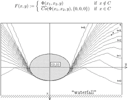
Caratheodory has described in [24] many examples of control problems. The problem we study here is derived from the so called Zermelo’s problem. Our aim is to illustrate how barriers can be characterized and computed as the boundary of the Viability Kernel.
The problem can be summed up as follows. Let ϕ(x1, x2) be the water current of a river at position (x1, x2).
The current is assume to be decreasing with the distance from the middle axis of the river
ϕ(x1, x2) := (1 − ax22, 0).
A swimmer aims at reaching an island but if he passes over some “waterfall” beyond the island, he completely fails. He is no more allowed to pass over the banks of the river. The swimmer has his own dynamic and he can swim in any direction at a speed c(t). Taking into account that the swimmer is getting tired as time increases, we suppose that the function c(·) is decreasing. Let us take for instance c(t) := 1
1+0.25t.
Also the global dynamic is given by (x0
1(t), x02(t)) = ϕ(x1(t), x2(t)) + c(t)v(t)
(27)
with v(t) ∈ B. The system is non autonomous and depends explicitly on time t. Let us introduce the variable y which represents the time and consider the following dynamic
(x01(t), x02(t), y0(t)) ∈ (ϕ(x1(t), x2(t)) + c(t)B, {1}) := Φ(x1(t), x2(t), y(t)),
Let C = {(x1, x2) ∈ IR2 | x21+ x22 ≤ 0.44} be the (closed) island, K = [−6, 2] × [−5, 5] × IR+ be the river and
a = 251.
These values of parameters are chosen such that the swimmer can go upstream close to the bank for low values of t - when the swimmer is not yet too much tired - since c(t) can be greater than ϕ(x1(t), x2(t)) whenever
x2(t) ≥ x?2= (1−c(t)a )
1 2.
Our aim is to compute the region of points from which the swimmer can reach the island in a finite time while remaining in K. The following Proposition allows to compute it thanks to the Viability Kernel Algorithm. Proposition 2.24 Let Φ be a Marchaud map and K a closed subset of X. Assume that V iabΦ(K) = ∅. Let C be
a closed target contained in K and set F (x) :=
½
Φ(x) if x /∈ C
Co [Φ(x) ∪ {0}] if x ∈ C
The VIability Kernel is precisely the set
In this example one can easily show that, if there is no island, since the swimmer is getting more and more tired, any trajectory would reach and pass over the “waterfall”. In other words, V iabΦ(K) = ∅ and then we can apply
Proposition 2.24 with x = (x1, x2) and
F (x, y) :=
½
Φ(x1, x2, y) if x /∈ C
Co(Φ(x1, x2, y), {0, 0, 0}) if x ∈ C
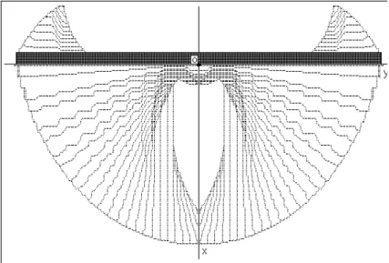
Figure 2: Intersections of the Viability Kernel with equidistant t-constant planes
Figure 2.4 shows the sections of the boundary of the Viability Kernel with equidistant t-constant planes. Figure 2.4 shows the boundary of the Viability Kernel which is the upper bound of the Viability Kernel. It can be interpreted as follows: any (x0
1, x02, t0) belonging to this boundary is such that, standing at position (x01, x02) at
a time t ≤ t0, the swimmer can reach the target in a finite time. If he is in late and passes at point (x0
1, x02) at any
time t > t0, he will never be able to reach the island and, so, he will disappear in a finite time. If he is at position
(x0
1, x02) exactly at a time t0, he will be able to reach the island providing that he never deviates from the limit
trajectory which follows the boundary of the viability kernel.
This corresponds to a semi permeable property of the boundary of the Viability Kernel (see [53], [57]).
On this figure we can observe for instance that, if the swimmer pass through point A at a time t > 3 then he will never be able to reach the island because he is already too tired. If he pass at a time t ≤ 3, he can reach the island.
3
The Minimal Time Function in Control Theory
We consider the following controlled system ½
x0(t) = f (x(t), v(t)), v(t) ∈ V for almost every t ≥ 0 (28)
where the state variable x belongs to a finite dimensional vector space X and V is a compact subset of some finite dimensional vector space.
Let C ⊂ X be a closed target and K ⊂ X be a closed set of state constraints.
Our propose is to characterize and to provide numerical schemes for computing the Minimal Time function ϑK C defined, for any initial condition x0, by:
ϑKC(x0) := inf
½
τ ≥ 0 | ∃x(·) solution to (28) with x(0) = xx(τ ) ∈ C and x(t) ∈ K ∀t ∈ [0, τ ]0
¾ (29)
Conventionnaly we set ϑK
C(x) = 0 if x ∈ C. Roughly speaking, ϑK
C(x) is the first time such that, starting from position x, the state of the system can reach the target C while remaining in the set of state constraints K. Note that ϑK
C takes values in IR+∪ {+∞} and that ϑK
C(x) = +∞ if no solution, starting from x, reaches the target C or if any solution, starting from x, leaves the constraints K before reaching the target.
In the sequel we denote by dom(ϑK
C) the domain of ϑKC: dom(ϑKC) := {x ∈ X | ϑKC(x) < +∞}. We recall now a regularity result for ϑK
C (see for instance [27]):
Proposition 3.1 If f : X × V → X is continuous, then the Minimal Time function ϑK
C satisfies the following properties:
a - for all x ∈ dom(ϑK
C), an optimal solution x(·) ∈ SF(x) exists such that ∀t ∈ [0, ϑK
C(x)), x(t) ∈ K and x(ϑKC(x)) ∈ C. b - the Minimal Time function ϑK
C(·) : X → IR+∪ {+∞} is lower semicontinuous on K. In particular, the epigraph6 of ϑK
C is closed. We denote it Epi(ϑKC). It is a subset of X × IR+. We shall denote by (x, y), with x ∈ X and y ∈ IR+ any element of X × IR+.
We first characterize the epigraph of the Minimal Time function as a viability kernel of a closed set for an extended dynamic and we deduce from this characterization a numerical scheme for computing ϑK
C.
3.1
Characterization of the Minimal Time function
As usually, we set F (x) :=Suf (x, u) and we replace control system (28) by differential inclusion (5). Then, if f is
continuous, F is Marchaud.
Let us define the expanded set-valued map Φ : X × IR Ã X × IR by: Φ(x, y) =
½
F (x) × {−1} if x /∈ C
Co((F (x) × {−1}) ∪ ({0} × {0})) if x ∈ C (30)
and consider the differential inclusion
(x0(t), y0(t)) ∈ Φ(x(t), y(t)), a.e. t ≥ 0 (31)
If F is a Marchaud map, Φ is also a Marchaud map.
Theorem 3.2 Let F : X Ã X be a Marchaud map, K and C be two closed subsets of X. We set H := K × IR+.
Then the epigraph of ϑK
C(·) is the viability kernel of H for Φ: V iabΦ(H) = Epi(ϑKC)
Proof of Theorem 3.2
Let (x, y) ∈ V iabΦ(H). We want to prove that y ≥ ϑKC(x). We can assume that x /∈ C since if x ∈ C, then y ≥ ϑK
C(x) = 0.
Let (x(·), y(·)) ∈ SΦ(x, y) be a solution which forever remains in H. We denote by θC(x(·)) ∈ [0, +∞] the first time that the solution x(·) reaches the target C:
θC(x(·)) := inf{t ≥ 0 | x(t) ∈ C}
From the very definition of Φ, on [0, θC(x(·))], (x(·), y(·)) is solution to the differential inclusion x0(t) ∈ F (x(t)) y0(t) = −1 x(0) = x, y(0) = y
Let us now recall that (x(·), y(·)) remains in H := K × IR+. Thus y(t) = y − t is not smaller than 0 on [0, θ
C(x(·))] and one has proved that y ≥ θC(x(·)). Moreover, the solution x(·) remains in K on [0, θC(x(·))]. So finally
ϑK
C(x) ≤ θC(x(·)) ≤ y In particular, x ∈ dom(ϑK
C) and (x, y) ∈ Epi(ϑKC). So we have proved that V iabΦ(H) ⊂ Epi(ϑKC) Conversely, let (x, y) ∈ Epi(ϑK
C). Since y ≥ ϑKC(x), then ϑKC(x) < +∞ and x ∈ dom(ϑKC). If x ∈ C, then (x, y) ∈ V iabΦ(H) because (0, 0) ∈ Φ(x, y).
Assume now that x /∈ C. From Proposition 3.1, there is a solution x(·) ∈ SF(x) such that x(t) ∈ K, ∀t ∈ [0, ϑKC(x)] and x(ϑKC(x)) ∈ C
Then let us define x?(·) and y?(·) as follows: (x?(t), y?(t) = ½ (x(t), y − t), ∀t ≤ ϑK C(x) (x(ϑK C(x)), y − ϑKC(x)) ∀t ≥ ϑKC(x) Since ϑK
C(x) ≤ y, then ∀t ≥ 0, y(t) ≥ 0. Since ∀t ≥ ϑKC(x), y0?(t) = 0 and since x?(t) ∈ C, then it is clear that the pair (x?(·), y?(·)) is a solution to system (31) starting from (x, y) and viable in H.
Thus we have proved that (x, y) ∈ V iabΦ(H). So
V iabΦ(H) = Epi(ϑKC)
Q.E.D.
3.2
Numerical approximation of the Minimal Time function
We now explain how the computation of V iabΦ(H) leads to a numerical scheme for approximating ϑKC. 3.2.1 Time discretization
Following the approximation method developped in section 2.2, we consider the finite difference inclusion system associated with Φ : X × IR+Ã X × IR+.
We have to define a time discretization Φε: X × IR+Ã X × IR+ which satisfies H0, H1 and H2. Let us define Φε(x, y) :=
½
{F (x) + (M `ε)BX} × {−1} if dC(x) > M ε Co [{(0, 0)} ∪ {F (x) + (M `ε)BX} × {−1}] otherwise
Lemma 3.3 If F is `−Lipschitz and bounded by some constant M (satisfying (11)), Φεsatisfies assumptions H0, H1 and H2.
Proof - Assumption H0 is clearly fulfilled because F is Marchaud and Lipschitz. Let us show that H1 is fulfilled with φ(ε) := 2M `ε.
Let ((x, y), (vε
x, vεy)) belong to Graph(Φε). There are two cases
- or dC(x) ≤ M ε. Then there exists some x0∈ C such that kx0− xk ≤ M ε. Thus (vε x, vεy) ∈ Co [{(0, 0)} ∪ {F (x) + (M `ε)BX} × {−1}] ⊂ Co [{(0, 0)} ∪ {F (x0) + (2M `ε)B X} × {−1}] ⊂ Φ(x0, y) + 2M `εBX×IR so that ((x, y), (vε
x, vyε)) belongs to Graph(Φ) + φ(ε)BX×IR.
For proving H2, let us fix (x0, y0) ∈ X × IR+. Let x ∈ X be such that kx − x0k ≤ M ε. Let us show that
Φ(x, y) ⊂ Φε(x0, y0), ∀y ∈ IR+. Indeed,
- if x /∈ C, then Φ(x, y) = {F (x)} × {−1} ⊂ {F (x0) + M `εBX} × {−1} ⊂ Φε(x0, y),
- if x ∈ C, then dC(x0) ≤ M ε, and F (x) ⊂ F (x0) + M `εBX and
Φ(x, y) := Co [(F (x) × {−1}) ∪ (0, 0)}] ⊂ Φε(x0, y)
Q.E.D. 3.2.2 State discretization
Let Φεbe the previous discretization of Φ and set Gε(x, y) := (x, y) + εΦε(x, y).
Let Rh be an integer lattice of IR generated by segments of length h and set Rh+:= Rh∩ IR+. Typically, Rh is a grid and is such that ½
i) Rh is stable by addition and substraction ii) ∀h, Rh⊂ Rh
2
(32)
As in subsection 2.3, we consider a discretization of the state space Xh× Rhwhere Xh satisfies (20). Let us set αεh:= α(ε, h) := 2h + `εh + M ε2.
We now define Γε,h as follows
Γε,h(xh, yh) := ({xh+ εF (xh) + αεhB} × {yh− ε + [−h, h]}) ∩ (Xh× Rh) if dC(xh) > M ε + h Co[{xh+ εF (xh) + αεhB} × {yh− ε + [−h, h]} ∪ {xh, yh}] ∩ (Xh× Rh) if dC(xh) ≤ M ε + h
Lemma 3.4 Assume that F is `−Lipschitz and bounded by some constant M . Then Γε,h is a “good discretization” of Gε satisfying H3 and H4.
The proof is the same as that of Lemma 3.3. Now applying Theorem 2.19 yields
Corollary 3.5 Suppose that the assumptions of Lemma 3.4 are fulfilled. Let Hh:= [(K + hB) ∩ Xh] × [R+h]. Then we have Lim ε→0+, h ε→0+ −→ V iabΓε,h(Hh) = Epi(ϑ K C) 3.2.3 The fully discrete approximation
From Corollary 3.5 we deduce a fully discrete scheme for computing the Minimal Time function ϑK C(·). Let εp∈ Rhp be a sequence converging to 0
+when p tends to ∞ such that hp
εp → 0
+. Moreover, we assume that
εp > hp. In practice, we can again choose hp and εp as previously given in (25). We also assume that εp, ∈ Rhp
and hp∈ Rhp.
Let us denote αp:= α(εp, hp) and Khp:= (K + hpB) ∩ Xhp.
Let us suppose that, starting at step p = 0 with the initial value T∞
0 ≡ 0, we have computed, from step k = 1
to step k = p − 1, the functions T∞
k : Khk → Rhk.
At step p, starting from T0
p = Tp−1∞ , we built recursively the sequence of functions Tpn: Khp → Rhp as follows
Tn+1 p (x) := ( εp− hp+ min v∈V b∈BT n p(x + εpf (x, v) + αpb), if dC(x) > M εp+ hp Tn p(x) otherwise (33)
This iterative process corresponds to the algorithm described in Proposition 2.18. The role played by Kn ε,h in the iterative construction given in Proposition 2.18 is played here by the epigraph of Tn
p. In particular: Lemma 3.6 For any x ∈ Khp, the limit
T∞ p (x) := limn→+∞Tpn(x) exists and Epi(T∞ p ) = −→ V iabΓε,h (Hh)
Proof of Lemma 3.6 : Let us set Γp:= Γεp,hp and let us consider the sequence of (discrete) sets A n defined as in Proposition 2.18 by A0:= Epi(T∞ p−1) and An+1:= {(x, y) ∈ An| Γ p(x, y) ∩ An6= ∅} We are going to prove by induction (on p and on n) that An= Epi(Tn
p) and that Tpn+1≥ Tpn. Note that for n = 0, the equality A0= Epi(T0
p) is obvious. Moreover, since Tp0:= Tp−1∞ ≥ 0 and since εp > hp, this proves that T1
p ≥ Tp0.
Suppose the result proved up to n. Then, for any (x, y) ∈ Epi(Tn+1
p ), one has : y ≥ ( εp− hp+ min v∈V b∈BT n p(x + εpf (x, v) + αpb), if dC(x) > M εp+ hp Tn p(x) otherwise
Assume that dC(x) > M εp+ hp and let v ∈ V , b ∈ B realize the minimum in the expression. Then (x + εpf (x, v) + αpb, y − εp+ hp) belongs to Γp(x, y) (from teh very definition of Γp) and to An:= Epi(Tpn) because
y ≥ εp− hp+ Tpn(x + εpf (x, v) + αpb) ≥ Tpn(x + εpf (x, v) + αpb) Moreover, (x, y) belongs to An because Tn+1≥ Tn. So, if d
C(x) > M εp+ hp, then (x, y) ∈ An+1. Otherwise, (x, y) belongs to Γp(x, y) and to An because y ≥ Tpn(x). So we have proved that Epi(Tpn+1) ⊂ An+1.
Conversely, if (x, y) belongs to An+1, and if d
C(x) > M εp+ hp, there are v ∈ V , b ∈ B, s ∈ [−hp, hp] such that (x + εpf (x, v) + αpb, y − εp+ s) belongs to An, i.e.,
y ≥ εp− s + Tpn(x + εpf (x, v) + αpb) ≥ Tpn+1(x)
One another hand, if dC(x) ≤ M εp+ hp, then (x, y) also belongs to An so that y ≥ Tpn(x) = Tpn+1(x). In both cases, we have proved that (x, y) belongs to Epi(Tn+1
p ). Thus the equality An+1= Epi(Tpn+1) is proved. We have finally to prove that Tn+2
p ≥ Tpn+1. If dC(x) ≤ M εp+ hp, this is obvious. Otherwise, Tn+2 p (x) = εp− hp+ Tpn+1(x + εpf (x, v) + αpb) ≥ εp− hp+ Tpn(x + εpf (x, v) + αpb) ≥ Tn+1 p (x) since Tn+1
p ≥ Tpn. So we have finally proved our claim. Since Tn
p(x) is non decreasing, it converge to some Tp∞(x) such that Epi(Tp∞) =
\ n
An=V iab−→ Γp(Hp)
from Proposition 2.18. Q.E.D.
Comments
• For a greater writing convenience, we extend maps Tn
p on the whole set X by setting Tpn(x) = +∞ whenever x /∈ Khp. Also, in this equation, since T
n
p is defined on the whole space X, the term Tpn(x + εpf (x, v) + αpb) takes finite values only at points x + εpf (x, v) + αpb which belong to the grid Khp for precise values of u and
b.
• Let us notice also that, for any x ∈ Khp and for any v ∈ V , there exists at least some b ∈ B such that
x + εpf (x, v) + αpb ∈ Khp. So maps T
n
p are well defined on Khp.
• The convergence can be accelerated when replacing the value of Tn
p(x + εpf (x, v) + αpb) in (33) by the value of Tn+1
p (x + εpf (x, v) + αpb) as soon as it has been already computed.
Now, exploiting the Refinement Principle stated in Theorem 2.23, we define the initial function T0
p+1 as follows Tp+10 (x) := ( −(hp+ hp+1) + min b∈B T ∞ p (x + (hp+ hp+1)b), if x ∈ Khp+1 +∞ otherwise
Corollary 3.7 If the assumptions of Theorem 2.23 are fulfilled, the sequence T∞
p converges to ϑKC in the epigraphic sense: Epi(ϑKC) = Lim p→+∞ Epi(T ∞ p ) Moreover, ∀xp∈ Rhp, T ∞ p (xp) ≤ ϑKC((xp)) and T∞ p converges pointwisely to ϑKC ∀x ∈ K, ϑKC(x) = p→+∞lim min xp∈(x+hB)∩Xhp Tp∞(xp)
The epigraphic convergence is a direct consequence of the convergence of fully discrete viability kernels to the continuous viability kernel (Theorem 2.19).
The pointwise convergence is a consequence of the same Theorem where the viability kernel and the fully discrete viability kernels are the epigraphs of functions ϑK
C and Tp∞. Let us define the set-valued map ˜T∞
p which epigraph is precisely Epi(Tp∞) + hBX×R. Then, on the one hand, we have
∀x ∈ K, ∃xp∈ x + hpB such that ˜Tp∞(x) ≤ Tp∞(xp) ≤ ˜Tp∞(x) + hp. From (23) stated in Theorem 2.19 we deduce that Limsup
p→∞
Epi( ˜T∞
p ) ⊂ Epi(ϑKC) and consequently ∀x ∈ K, ϑKC(x) ≤ lim infp→∞,x0→xT˜p∞(x0) ≤ lim infp→∞ min
kxp−xk≤hp
Tp∞(xp)
On the other hand, from (22) stated in Theorem 2.19, which is written Epi(ϑK
C) ⊂ Epi( ˜Tp∞), we have ˜ T∞ p (x) ≤ ϑKC(x). and thus min xp∈x+hpB T∞ p (xp) ≤ ϑKC(x) + hp so that lim sup p→∞ xp∈x+hminpB T∞ p (xp) ≤ ϑKC(x) In conclusion we have lim
p→∞xp∈x+hminpB
T∞
p (x) = ϑKC(x). Q.E.D.
3.2.4 Outline of the Algorithm
Procedure of Construction of the data (parameter p)
Rhp← 2
−pZZ, X hp ← 2
−pZZN. {Definition of the grids R
hp and Xhp.}
hp← 2−p, εp = p
hp/M ` {Definition of steps hp and εp∈ hpZZ}
αp ← 2hp+ `εp(hp+ M εp) {Definition of the dilation term.} Khp← (K + 2 −pB) ∩ X hp {Definition of Khp} Initialization p ← 1 if x ∈ K1 then T0 1(x) ← 0 else T0 1(x) ← +∞
Main loop Minimal Time Problem For p := 1 to ¯p do
n := 0
Repeat {Beginning of calculus of T∞
p }
x ← xp↓ {xp↓ is the first point of the grid Khp}
Repeat {Scanning of the grid}
if dC(x) > M εp+ hp then Tn+1 p (x) ← [εp− hp+ min v∈V,b∈BT n p(x + εpf (x, v) + αpb)]
else Tn+1
p (x) ← Tpn(x)
x ← N ext(x) {N ext(x) is the following point of the grid}
until x ≡ xp↑ {xp↑ is the last point of the grid}
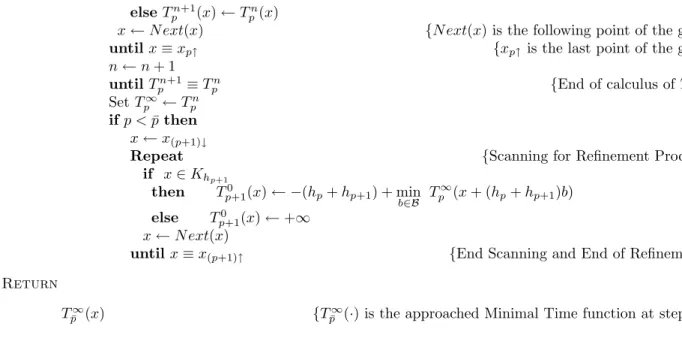
n ← n + 1 until Tn+1 p ≡ Tpn {End of calculus of Tp∞} Set T∞ p ← Tpn if p < ¯p then x ← x(p+1)↓
Repeat {Scanning for Refinement Process}
if x ∈ Khp+1 then T0 p+1(x) ← −(hp+ hp+1) + min b∈B T ∞ p (x + (hp+ hp+1)b) else T0 p+1(x) ← +∞ x ← N ext(x)
until x ≡ x(p+1)↑ {End Scanning and End of Refinement}
Return
T∞
¯
p (x) {Tp¯∞(·) is the approached Minimal Time function at step ¯p }
3.3
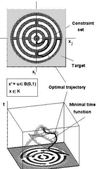
Minimal Time for a basic target problem with constraints
Let us consider the basic example described by the following dynamic:½ x0 1(t) = cvx1 x0 2(t) = cvx2 with v 2 x1+ v 2 x2 ≤ 1
Let C = {(x1, x2) ∈ IR2| x21+ x22≥ 8} be the target and K the constraint of labyrinth shape as shown on the
figure.
Figure 3.3 down represents the minimal time function obtained for a final space discretization step h = 10−3.
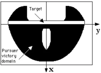
3.4
Minimal Time for the swimmer problem with obstacles
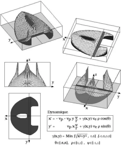
Let us come back to the previous Zermelo’s type problem but, now, in presence of obstacles. The swimmer aims at reaching the island in minimal time. His dynamic now is autonomous. It is described by through the following system: x0 1(t) = (1 − ax22) + vx1 x0 2(t) = vx2 with v 2 x1+ v 2 x2≤ c 2 (34)
where C = {(x1, x2) ∈ IR2 | x21+ x22 ≤ 0.44} and K = {[−6, 2] × [0, 5]}\M × IR+. The set M is the union of a
triangular and a square shapes as viewed on figure 3.4.
Barriers appear corresponding to discontinuities of the Minimal Time function.
4
Qualitative Differential Game Problems: the target problem
We investigate differential games with dynamic described by the differential equation ½
x0(t) = f (x(t), u(t), v(t)), u(t) ∈ U, v(t) ∈ V
(35)
where f : X × U × V → X, U and V being the control sets of the players.
Throughout this section, we study the following game. O ⊂ X is an open target (for the first player) and E ⊂ X a closed evasion set (for the second player). The first player - Ursula, playing with u - aims at reaching O in finite time while avoiding E and the second player - Victor, playing with v - aims at avoiding O until reaching E. This game is called the target problem.
The aim of the section is to explain how to characterize and to compute the set of initial positions from which a player may win, whatever his adversary plays. This set is called the victory domains of the player. The charac-terization is given by an extension of the Viability approach to the more general framework of differential games.
Figure 6: Level Curves of the Minimal Time function for Zermelo problem with obstacles and visualization of the optimal swimming policy