HAL Id: hal-01276913
https://hal.inria.fr/hal-01276913
Submitted on 22 Feb 2016
HAL is a multi-disciplinary open access
archive for the deposit and dissemination of
sci-entific research documents, whether they are
pub-lished or not. The documents may come from
teaching and research institutions in France or
abroad, or from public or private research centers.
L’archive ouverte pluridisciplinaire HAL, est
destinée au dépôt et à la diffusion de documents
scientifiques de niveau recherche, publiés ou non,
émanant des établissements d’enseignement et de
recherche français ou étrangers, des laboratoires
publics ou privés.
How much does a VM cost? Energy-proportional
Accounting in VM-based Environments
Mascha Kurpicz, Anne-Cécile Orgerie, Anita Sobe
To cite this version:
Mascha Kurpicz, Anne-Cécile Orgerie, Anita Sobe. How much does a VM cost? Energy-proportional
Accounting in VM-based Environments. PDP: Euromicro International Conference on Parallel,
Dis-tributed, and Network-Based Processing, Feb 2016, Heraklion, Greece. pp.8, �10.1109/PDP.2016.70�.
�hal-01276913�
How much does a VM cost?
Energy-proportional Accounting in VM-based
Environments
Mascha Kurpicz
∗, Anne-C´ecile Orgerie
†and Anita Sobe
∗∗University of Neuchatel, Switzerland - Email: {mascha.kurpicz, anita.sobe}@unine.ch †CNRS, IRISA, France - Email: [email protected]
Abstract—The costs of current data centers are mostly driven by their energy consumption (specifically by the air conditioning, computing and networking infrastructure). Yet, current pricing models are usually static and rarely consider the facilities’ energy consumption per user. The challenge is to provide a fair and predictable model to attribute the overall energy costs per virtual machine (VM). Current pay-as-you-go models of Cloud providers allow users to easily know how much their computing will cost. However, this model is not fully transparent as to where the costs come from (e.g., energy). In this paper we introduce EPAVE, a model for Energy-Proportional Accounting in VM-based Environments. EPAVE allows transparent, reproducible and predictive cost calculation for users and for Cloud providers. We show these characteristics of EPAVE by a number of use cases in heterogeneous data centers and discuss the applicability of EPAVE.
I. INTRODUCTION
The trend of computing in the Cloud grows, which conse-quently requires bigger data centers, more processing power and hence more CPUs. Whereas the hardware gets more and more energy-efficient the overall energy consumption of data centers increases. Actually, today’s Cloud computing requires more electricity in the form of energy than entire countries such as India or Germany [1].
It is hence not surprising that energy represents one of the main cost factors of a data center. The major energy consumers are the air conditioning, the network infrastructure (routers, switches) and the servers [2]. However, these costs are rarely reflected in the attribution of energy consumption to a single consumer (e.g., a virtual machine).
As users share the same resources on a single node, most of the existing models concentrate on attributing the power consumption of this shared node to a single consumer. For instance, how much of the CPU power consumption can be related to a VM [3], [4], [5]?
Our vision is to consider energy accounting on the data center level to enable pricing models where every user will pay for the actual usage of resources. The challenge is to provide a fair attribution model that is predictable to provide incentives for energy-efficient computing in the Cloud.
Hence, in this paper, we introduce EPAVE (Energy-Proportional Accounting in VM-based Environments) for re-alizing accounting of real energy costs of the data center to each client considering the major consumers and the entire
facility costs. More specifically, we target energy proportional accounting for each virtual machine (VM).
Context: Currently the relation between IT infras-tructure and facility energy costs are modeled with the Power Utilization Efficiency (PUE) metric. This metric is used to help operators on decisions regarding new hardware infrastructure. E.g., Google measures the PUE per site each three months1for
each of its data centers. While the PUE is a useful metric for reflecting the overall efficiency of a data center, its applicability for the day-to-day operation of the data center is limited because it does not grasp the variability of the actual power consumption of the data center.
In a data center, the instant power consumption can be divided into static and dynamic parts. The static parts are the base costs of running the data center when being idle; the dynamic costs depend on the current usage. In an ideal case, the overall power consumption would be proportional to the utilization of the hardware (power proportionality). However, having non-negligible static parts, power proportionality is not yet achievable [6]. Nonetheless, we can get closer to power proportionality by accrediting the static power parts to each application, depending on the time and the resources used. Since time plays a major role, we will focus on energy instead of power consumption (an instant measure). Hence, we talk rather about energy proportionality than power proportionality. Challenges: Dynamic power consumption mainly de-pends on the resources which are used: computing, storage, networking resources. In the case of virtual environments, the hardware resources may be shared among different users and different virtual machines, if they run on the same host. In this context, a power-aware model needs to estimate the relative utilization per user to attribute the dynamic costs of the physical resources to a particular VM.
The static costs have to be considered at different levels: • at the data center level: power delivery
nents, cooling systems, other miscellaneous compo-nents such as data center lighting. This part is captured by the PUE.
• at the resource level: idle power consumption of servers and routers.
The main challenge we tackle in this paper is to divide
the static costs among the users in a fair and predictable way, considering the actual utilization of the resources per VM.
Motivating example: The first simplistic model com-ing to mind is to share the idle power consumption of a server proportionally among the VMs it is currently hosting. However, such a model raises several issues. First, the costs of a VM are strongly linked to the utilization of the physical host, which depends on the hypervisor and the OS scheduler, and not on the user. For instance, if a VM stops, the costs of each VM on the same host suddenly increase. Moreover, identical VMs (same type) performing the same work may have different costs depending on the physical host they are scheduled on and on other work currently performed on the host.
Therefore, a more elaborated model is required for our purpose. Inspired by the PUE, a first attempt could be to calculate an effectiveness ratio per server. As an example, let us consider one of the Grid’5000 servers, namely Taurus. Grid’5000 is a large-scale and versatile testbed for experiment-driven research in all areas of computer science, with a focus on parallel and distributed computing including Cloud, HPC and Big Data [7]. The Taurus server is a Dell PowerEdge R720 which has two 6-cores Intel E5-2630 processors, 32 GB of RAM and two 300 GB hard disks. This server is plugged to an external powermeter providing one instantaneous power measurement per second with an accuracy of 0.125 Watts. The measured idle power of this server is 95 Watts.
For the calculation, we take into account power values we measured over a one-year period (between 1st of April 2014 to 1st of April 2015). For this period of time, the maximum observed power consumption is 217 Watts, and the average power consumption is 103 Watts.
We define the utility ratio (inspired by the PUE) as the average power consumption for the period of one year over the useful power consumption (average minus idle):
U tilityavg=
Pavg
Pavg− Pidle
= 103
(103 − 95) = 12.875 In this case, for Taurus, the utility ratio is 12.875. When taking the maximum power consumption as a basis the utility ratio is 1.8. These figures mean that for each useful Watt spent, we actually spend 12.875 W on average (only for this server, not considering the air conditioning and so on). And we would consume 1.8 W per useful Watt if the utilization was maximal for this server.
The gap between a ratio of 12.9 and 1.8 is large, and this clearly shows the importance of idle part over the overall power consumption under realistic workloads. As it is an important factor in the electricity budget of a data center, it needs to be carefully integrated into a power-aware attribution model for VMs.
Using the utility ratio as a basis for attribution of costs can be seen as unfair for the users as it strongly depends on the server utilization. A VM scheduled to a server with low utilization will have higher costs. On the other hand, using the maximal utility ratio does not reflect the reality of the data center utilization, and thus, the real electricity bill paid by the provider.
Contribution: In this paper, we propose, EPAVE, a power-aware attribution model for VMs taking into account the overall consumption of the data center hosting them. The model covers heterogeneity of nodes as well as heterogeneity of VMs regarding their reservations.
Organization: This paper is organized as follows. Section II presents the related work. The EPAVE model is detailed in Section III. Use cases of this model are described in Section IV. We discuss the properties of the model in Section V and provide an outlook on the usage of EPAVE in Section VI. Finally, Section VII concludes the paper.
II. RELATED WORK
Benefiting from economies of scale, Cloud infrastructures can effectively manage their resources and offer large storage and computing capacities while minimizing the costs for users. However, the rapid expansion of these infrastructures led to an alarming and uncontrolled increase of their power consump-tion. For instance, in 2010, the services offered by Google were based on 900,000 servers that consumed an average of 260 million Watts [8].
Moving from instrumenting to modeling the energy con-sumption is a tough but necessary task in order to improve the energy efficiency of distributed infrastructures. It is indeed essential to understand how the energy is consumed to be able to design energy-efficient policies.
A. Resource-based models
Most of the models found in literature split the con-sumption of an entire server into the concon-sumption of each component of the server [3] or consider that consumption is proportional to the load [9]. Several studies are focused on modeling the energy consumption of particular components: CPU [10] influenced by the frequency, voltage and workload, network card [11] with costs per packet and per byte, and disk [12] driven by the rotational speed and the read and write operations.
However, we have shown in [13] the limits of these approaches for modeling the energy consumption of entire servers under various workloads. Concerning the experimental approaches found in literature, they mainly consider just one type of machine, or even only one type of application [13]. So, it is necessary to design unified models closer to reality. Con-cerning the consumption of entire infrastructures, the authors of [14] show that computing resources represent the biggest part in Clouds consumption. An alternative approach [15] shows that, depending on the studied scenario, the energy costs of the network infrastructure that links the user to the computing resources can be bigger than the energy costs of the servers.
As shown in [13], simple models are not convincing in the general case and especially for multicore architectures – which tend to become widespread. It is therefore necessary to depend on benchmarks for the development and validation of reliable energy cost models for these heterogeneous resources. These benchmarks need to propose several kinds of workloads: computation-intensive, disk-intensive, etc.
B. VM models
Virtualization adds another layer of complexity and soft-ware power models are needed because it is not possible to attach a power meter to a virtual machine [16]. In general, VMs can be monitored as black-box systems for coarse-grained scheduling decisions, e.g., as done with Joulemeter [4]. If we want to be able to do fine-grained scheduling decisions—e.g., with heterogeneous hardware—we need to be able to consider finer-grained estimation at sub-system level and might even need to step inside the VM.
Bertran et al. [17] propose an approach that uses a sampling phase to gather data related to performance-monitoring coun-ters (PMCs) and compute energy models from these samples. With the gathered energy models, it is possible to predict the power consumption of a process, and therefore apply it to estimate the power consumption of the entire VM. This is similar to the work presented by BitWatts [5], which is further capable of estimating the power consumption of a process running within a VM and supports CPU-specific features such as hyperthreading and turbo frequencies.
Another example is given by Bohra et al. in [3], where the authors propose a tool named VMETERthat estimates the consumption of all active VMs on a system. A linear model is used to compute the VMs’ power consumption with the help of available statistics (processor utilization and I/O accesses) from each physical node. The total power consumption is subsequently computed by summing the VMs’ consumption with the power consumed by the infrastructure.
C. Idle power consumption
The idle power concerns the power consumed by an infrastructure which is powered on but not running any task. Typically, for a server, it consists of the energy consumed while idle, but fully powered on. This consumption depends on the hardware of the server, but it can also depend on the operating system installed on it as it is responsible for the background tasks running continuously on the server (like monitoring tasks). This power is usually not taken into account by VM-based models described in the previous section. For an entire data center, the idle power consumption includes all the power which does not depend on the workload.
Often only the power consumption of IT equipment is considered although air conditioning can consume 33% of the global power needed by a data center [18]. This cost can be reduced by free cooling techniques exploiting outside air [19]. The power consumption of such cooling techniques is tightly correlated to the weather, and thus vary over time even if the workload does not vary. Therefore, their power consumption, which is considered to belong to the static idle part, can vary over time.
Most of the studies do not use the same definition for the energy costs of the computing infrastructure: for instance, the network used to link the computing resources is not taken into account most of the time. In the same way, as surveyed in [2] some works take into account only the dynamic consumption of the machines and not their static consumption (correspond-ing to the consumption when machines are powered on but idle) which can yet represent more than half of the total
power consumption. In our context, we will consider all the equipment operated by the Cloud provider: the data centers (including cooling infrastructures) and the network links inside and between the data centers.
In addition to these considerations, simply measuring the power consumption of computing resources may pose prob-lems of security and confidentiality as identified in [20]. Indeed, it is shown that by simply having access to the energy consumption of a cloud server, one can guess with high probability what type of application, among various possible, was running in its virtual machines. It is therefore necessary to consider an instrumentation of these platforms that guarantees the privacy of the user, of the provider regarding its machines, and of the applications. This is why our model do not rely only on direct measurements on the physical machines: because it would reveal too much information. For instance, it could reveal the server’s position in the rack as it influences the power consumption due to the air conditionning situation [13].
III. EPAVE
The key idea of EPAVE is to attribute the data center’s static and dynamic costs (C) to each VM, which can be then used as a basis for several use cases as described later. As costs we consider the total consumption (Ctotal) during the
execution of a VM in the context of a data center. Ctotal= Cstatic+ Cdynamic
The static costs comprise the idle consumption of each node and the idle consumption of the routers as well as induced consumption of the entire data center (routers, air conditioning, power distribution units, etc.). To cover the entire data center the Power Usage Effectiveness (PUE) has become the industry-preferred metric for measuring infrastructure energy efficiency for data centers [21], [22]. It is defined as the ratio of total facilities energy to IT equipment energy:
P U E = T otal F acility Energy IT Equipment Energy
Therefore, we will use the PUE to account for the con-sumption part exterior to the IT equipment itself which is already taken into account. As outlined in the data center industry survey conducted by Uptime Institute Network (a user group of large data center owners and operators) [22], the adoption of PUE is rising worldwide, and its measurement and improvement are widely targeted by the 1,000 surveyed data center operators and IT practitioners. That is why we believe that the PUE metric is easily accessible for Cloud providers for their data centers. From the PUE definition, for 1 Watt consumed by the IT equipment, the entire data center infrastructure consumes in fact 1 × P U E Watts. Therefore, the static costs of a data center have to be multiplied by the data center’s PUE: Cstatic= #nodes X Cidlenode+ #routers X Cidlerouter ! · P U E The dynamic costs include the dynamic energy consump-tion part of the servers, routers and storage devices, which we can formulate as a weighted sum of the individual costs. The
weights represent the resource usage of the current workloads, which can be between 0 and 1, where 1 means maximum utilization of the given resource and 0 means no utilization.
Cdynamic= α · Ccomp+ β · CIO+ γ · Cnet
To attribute the overall costs to a single VM, we first need to distribute the idle costs in a fair and transparent manner. In many cases the idle costs (or idle power consumption) are only divided by the number of VMs [3]. However, for energy-proportional accounting it is necessary to consider the size of a VM, and in particular, its number of vCPU as CPU is the most consuming device in a server [2]. Inspired by the VM types chosen by Amazon we will differentiate VMs by the number of their assigned virtual CPUs. In addition we want to take into account heterogeneous data centers.
The dynamic costs are determined when the VM finishes by using the real resource utilization of the physical resources. The total costs are limited to the static costs as the lower bound, and on the maximum consumption as the upper bound. Reporting these bounds to the user makes the final VM’s costs predictable (bounded) and keeps the spirit of the pay-as-you-go manner although the dynamic part of the costs are in most cases smaller than the static parts (reflecting the reality of the power consumption of typical data center servers).
To sum up, the maximum costs of a VM grow with its size as shown by an illustrative example in Figure 1. In this experiment we were inspired by the Amazon VM sizes. The static costs, Cstatic(VM), depend on the number of cores
reserved by the VM, and the dynamic costs Cdynamic(VM)
on the actual usage (in our case performed by the stress command). In more details, we model the static and dynamic costs per VM as described in the following paragraphs.
Small Medium Large XLarge 2XLarge
Costs per VM
Static costs Dynamic costs
Fig. 1. Example of maximum costs distribution among different types of VM
Static costs: As we want these costs to be static and independent from the hypervisor, we use a weighted averaged value of the idle power consumption of all the servers. This model is similar to the one currently in application at Ama-zon [23]: the costs are proportional to the number of virtual CPUs (vCPU) assigned to the VM:
Cstatic(VM) =
#vCP U (VM) P#nodes
#CP U (node) · Cstatic Dynamic costs: The dynamic costs are hardware and application dependent and require monitoring. According to [24] the acceptance of dynamic models is increased if the
costs are limited by an upper bound. Indeed, a VM cannot exceed the physical resources allocated to it (CPU, RAM and disk mainly), so the upper bound can be determined for each type of VM over each type of physical node. The actual dynamic costs per VM will be in the range of 0 (idle) and the maximum resource usage. The challenge is to attribute the maximum dynamic costs to a VM. In general the dynamic costs of a VM are the measured or estimated energy consumption (E), which is the integral of the power consumption (P) measured/estimated per time unit (T).
Cdynamic(VM) = E(VM) =
Z T
0
P (VM) dt
In general, a VM cannot consume more than the maximum dynamic costs of the entire server (Cdynamic). If the VM
is co-located with other VMs it is necessary to split up the dynamic costs. Here, we use a very simple model to define an approximate upper bound for the costs of a VM, by using the number of cores the VM got assigned as a basis. Note that the focus on the number of vCPUs (ignoring the disk and network) is chosen because the number of vCPUs usually differentiates VM sizes offered by Cloud providers. Additionally, the CPU is one of the highest power consumers on a node.
0 ≤ Cdynamic(VM) ≤
#vCP U (VM)
#CP U (node)· Cdynamic(node) An alternative would be to use a software power estimation model that is capable of attributing the dynamic costs to a VM, such as VMeter [3], or Bitwatts [5].
IV. USE CASES
In this section, we showcase how to calculate Cstatic(VM)
and Cdynamic(VM) based on real-world experiments. Based
on the real data we can use EPAVE to estimate the costs of different use cases.
For the experiments, we rely on selected nodes from the Grid’5000 cluster to which powermeters are attached [7]. Specifically, we performed the experiments on two kinds of nodes, Taurus and Sagittaire, whose characteristics are specified in Table I. We further consider different sizes of VMs, which are inspired by the Amazon instances and shown in Table II.
A. Homogeneous setup
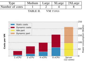
Figure 2 presents the costs Ctotal(VM) for a homogeneous
cluster with Taurus servers with 12 cores each. Their average idle power consumption is 95W per server. In a real setup the calculations need to include network costs and PUE, hence we need to add the costs for a number of switches (approx. 350W each) and multiply by the PUE (e.g., 1.22). In this specific example, we demonstrate the cost models based on the idle power of the servers as a matter of simplification for the calculations. The static costs per core are easy to compute: 95/12 = 7.92. The dynamic part represents the maximal achievable dynamic power consumption when running the stress command. Together these costs represent the upper bound of costs per VM. We can see that the static costs increase proportional to the number of cores assigned to the
Hardware Model Cores/Threads RAM (GB) TDP (W) # Servers Taurus: Dell PowerEdge R720 Intel Xeon e5-2630 (2.3GHz) 2x6/12 32 2x95 16 Sagittaire: Sun Fire V20z AMD Opteron 250 (2.4GHz) 2/2 2 215 79
TABLE I. HARDWARE CHARACTERISTICS OF THE SELECTED SYSTEMS
VM and two VMs having together 12 cores will reach the same static costs as the machine itself. Hence, in a homogeneous setup EPAVE would fall back to a trivial model, where only the upper bound of costs Ctotal(VM) have to be reported.
Type Medium Large XLarge 2XLarge Number of cores 1 2 4 8
TABLE II. VMTYPES
1 vCPU 2 vCPU 4 vCPU 8 vCPU Server (12 cores) 0 50 100 150 200 250
Power consumption (Watts)
Costs per VM
Static costs Dynamic costs Idle part Dynamic part
Fig. 2. Example of maximum cost distribution among different types of VM for a homogeneous cluster
B. Heterogeneous setup
If we switch to a heterogeneous use case (as shown in Figure 3) and run again the stress command, the static costs are not proportional anymore to the number of virtual cores as the idle power of the machines might be unbalanced. We showcase the unbalanced scenario with experiments performed on two different kinds of servers, whose characteristics are summarized in Table I. The two clusters are heterogeneous in terms of server architecture, but also in terms of number of nodes, and number of cores per node. The idle power consumption represents the average power consumption of a server over the entire cluster.
In this use case we can calculate the static costs for a one-vCPU VM as follows: Cstatic(V M ) = 1 P#nodes #CP U · #nodes X Cidlenode = 16 · 95 + 79 · 215 16 · 12 + 79 · 2 = 52.87
These costs are more than 6 times higher than in the homogeneous case with only Taurus nodes, but they represent half the costs of a cluster with only Sagittaire nodes. Therefore, heterogeneity among nodes leads to average static costs per virtual CPU which can be far from the costs per cluster. However, this is a healthy property of EPAVE: in order to cover the real energy costs with this accounting, the Cloud provider has to favor the utilization of the most energy-efficient servers. Dynamic costs present a similar behavior.
1 vCPU 2 vCPU 4 vCPU 8 vCPU Taurus
(12 cores)Sagittaire (2 cores) 0 100 200 300 400 500 600
Power consumption (Watts)
Costs per VM
Static costs Dynamic costs Idle parts Dynamic parts
Fig. 3. Example of maximum cost distribution among different types of VM for a heterogeneous cluster with unbalanced idle power for the server architectures
C. Underutilization of reserved resources
To show the applicability of our models, we performed experiments using real-world applications on a Taurus node. We installed Hadoop Yarn [25] on each of the nodes and ran sort and wordcount from the HiBench [26] benchmark suite. We run the workloads within a VM to be able to limit the number of cores they use in total. We started the VM once with only a single core, and once with all cores available. T This experiment is the basis for three use cases, where we want to showcase the effects of underutilization of reservations. Note that the dynamic costs are always measured in real experiments and the static costs are predetermined based on the idle power consumption.
The workloads have different power consumption patterns as shown by the example of the wordcount workload executed on all available cores in Figure 4. The idle power of the Taurus nodes is 95W. We also know the maximum total power of 220W, and 125W as basis for Cdynamic for all reserved cores
without idle power. These values can be predetermined and have to be collected only once per architecture. The actual dynamic costs of the workload vary between 0 and 100W over a runtime of 200 seconds. This shows the necessity of considering energy rather than power consumption, as we need to provide models that reflect the actual usage of the VM over time.
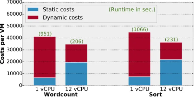
If we consider the pay-as-you-go model as a basis, a VM would cost according to its size (i.e., resources reserved) and according to the time used. The same idea is followed by EPAVE, but we consider both static and dynamic energy as a basis of costs. As an example, for the single core experiment, we calculate Ctotal(V M ) according to our model and fill it
with values from our experiments.
Ctotal(V M ) = Cidle∗ ratiovCores∗ runtime + Cdynamic
As shown in Figure 5 the static costs for using only a single core are smaller. However, because the single core is used for a longer time span, the dynamic costs are much higher leading to higher total costs than if all cores are used and reserved.
0 50 100 150 200 Time (seconds) 0 50 100 150 200
Power consumption (Watts)
Idle
Wordcount experiment Full load
Dynamic part
Fig. 4. Power profile of the wordcount workload using all available cores
1 vCPU 12 vCPU 1 vCPU 12 vCPU
0 10000 20000 30000 40000 50000 60000 70000
Costs per VM
Wordcount
Sort
(951) (206) (1066) (231) Static costsDynamic costs (Runtime in sec.)
Fig. 5. Costs of two parallel workloads with a reservation of one core and twelve cores
Let us consider a use case where the workload is not optimized for parallelization, but still the reservation covers all of the cores. If a workload only uses a single core out of 12, the dynamic costs will not change in comparison to the former use case, however, the static costs are distributed among the number of cores served. Taking the dynamic costs of the former experiment as a basis, this would mean a significant increase in costs for the VM (see Figure 6). In an ideal case a user is encouraged to reserve resources according to the resources required and parallelization capabilities of the workload.
The runtimes of the former experiments are rather low and we assumed that the reservation for a VM ends with the end of the workload. However, in reality most VMs are reserved for a given time span. For instance, if we consider the default minimum reservation of VMs of around 20 minutes the cost
12 vCPU
(1 used) 12 vCPU 12 vCPU(1 used) 12 vCPU
0 25000 50000 75000 100000 125000 150000 175000 200000
Costs per VM
Wordcount
Sort
(951) (206) (1066) (231) Static costsDynamic costs (Runtime in sec.)
Fig. 6. Costs of two workloads with underutilization of reserved cores
1 vCPU 12 vCPU 1 vCPU 12 vCPU
0 25000 50000 75000 100000 125000 150000 175000 200000
Costs per VM
Wordcount
Sort
(1200) (1200) (1200) (1200) Static costsDynamic costs (Runtime in sec.)
Fig. 7. Costs of two workloads with predetermined reservation time of 20 minutes per VM
distribution for the same workloads changes and the results are depicted in Figure 7. Hence, if we reserve all cores for 20 minutes but only use them for the first few minutes the static costs exceed the dynamic costs and the single core reservation is much more advantageous.
With EPAVE it is possible for a user to identify such discrepancies and decide for what kind of reservation is useful. Another possibility is to provide a recommendation service by the Cloud operator to provide incentives for energy-efficient resource reservation.
V. DISCUSSION
EPAVE keeps the philosophy of the Cloud: the pay-as-you-go model but based on energy consumption. The costs of a VM indeed depend on the physical resources reserved for it (static costs) and on the utilization made of these resources (dynamic costs). Moreover, the energy costs of a VM are predictable for the static part, and bounded for the dynamic part (bounded by the maximum costs as shown in Figures 2 and 3). Thus the user knows the maximal costs of the VM, and is able to estimate the real costs if the behavior of the running application and their energy consumption is known.
EPAVE is not designed to account for the real cost of a given VM as it could be measured by external wattmeters during the entire lifetime of this VM. In this case, the cost of a VM would be influenced by cloud provider operations like VM migration or allocation of other VMs on the same host. This does not seem to be a desirable feature as it would reveal private information from the provider point of view. This is why EPAVE is not based on this purely measurement technique and also why its goal is not to provide real measured costs but predictable, bounded, energy-proportional costs of a VM. These reflect the energy costs of an average VM of a given size hosted on a fixed Cloud platform, similarly to what is done for pricing models [23].
EPAVE provides a complete view of the energy costs related to the hosting of virtual machines. Indeed, it does not only take into account server-related costs, but also the costs of the air conditioning, the networking devices, the power supplies, etc. That is why EPAVE can help the Cloud provider to easily and fairly distribute the energy consumption of its entire infrastructure over the customers.
The computation of the energy costs determined by EPAVE relies, for the static side, on external power measurements
(PUE, idle power of the servers), and for the dynamic side, on wattmeters or software-based tools. If these measured information are stored over time, the EPAVE energy costs can be re-computed later, thus becoming verifiable and auditable. EPAVE encourages users to dimension adequately their VMs. Indeed, if a user is asking for a 4 vCPUs VM, but uses only 2 vCPUs, the two unused vCPUs will still be taken into account into the static costs – although their dynamic costs will be zero, and even if the Cloud provider is applying over-commitment of resources. The user is also encouraged to be energy-efficient on its utilization of the resources. Indeed, the dynamic costs are directly measured from the hardware, so all energy saving mechanisms employed by the user (e.g., energy-aware software) will be directly translated into a reduction of the dynamic costs of the VM. We assume here that the energy costs of a VM have somehow repercussions for the user (like a bonus-malus system, or monetary costs for VMs taking into account the energy).
On the other side, EPAVE encourages the Cloud provider to consolidate its VMs on a fewer number of nodes and to switch off the idle nodes. Indeed, the static costs for a physical server are divided into its potential number of virtual CPUs, thus assuming that all the cores are utilized by VMs to cover its entire energy consumption. For instance, for the Taurus servers described on Figure 2, the idle power consumption is about 95 Watts and they have 12 cores. Hence, the static costs for a 4 vCPU VM is 31.68 Watts, and for a 8 vCPU VM, it is 63.36 Watts. If these two VMs are hosted on the same server, they account for the entire idle power consumption of the server. However, if they are allocated to two different servers not hosting any other VM, only half of the static costs will be covered for these two servers.
In the case of heterogeneous servers, EPAVE encourages the Cloud provider to use the most energy-efficient nodes. For instance, for the case described in Figure 3 with the Taurus cluster and the old Sagittaire cluster, a VM with 2 vCPUs will have static costs of 105.74 Watts. So, its static costs are bigger than the idle power consumption of a Taurus server, which is still able to host 5 more of such VMs. However, this VM’s static costs are nearly twice smaller than the idle power consumption of a Sagittaire server which cannot host any additional VM.
VI. OUTLOOK
This section gives a non-exhaustive outlook on the appli-cation of EPAVE, and more generically of the utilization of energy-aware cost models.
A. Pricing models
EPAVE can serve as the basis for energy-aware pricing models. The static part is known at the beginning as it is defined by the VM type. For the dynamic part, the minimal bound is zero, and the maximal bound (for maximal energy consumption) can be provided to the user before the purchase. Reporting these bounds to the user makes costs per VM predictable (bounded) and keeps the spirit of the pay-as-you-go model because the dynamic part of the costs are in most cases smaller than the static parts (reflecting the reality of the power consumption of typical data center servers).
EPAVE can also serve as a basis for an energy-aware pricing model. The costs per VM as determined by EPAVE can be multiplied by a financial cost per kWh, and these financial costs can evolve over time to reflect market-based night and day prices of electricity providers for instance.
B. SLA with renewable energy sources
Service Level Agreements (SLAs) provide quantified guar-antees to the users concerning quality of service on the re-served VMs. In [27], the authors define green SLA: an explicit SLA for the percentage of renewable energy used to run the clients’ workloads. In [28], the terms of green SLAs include also the energy costs of networking devices and virtual links between VMs. The green SLA is negotiated between the IaaS provider and each client depending on its needs. Such an SLA requires to have quantifiable green cloud services [27]. That is to say, the provider has to know the energy consumption of each VM and the electricity mix employed by the data centers. EPAVE can be used here to determine the energy budget spent by the VMs of a given user, and thus, to deduce the amount of green energy required for the Cloud provider in order to fulfill the SLA conditions for this user.
C. User-oriented utilization
On the user side, EPAVE can be used as an energy cost metric in order to evaluate the energy-efficiency of a given application running on given VM configuration. This metric can be used in combination with the classical metrics (duration, performance, QoS, etc.). By extrapolation, EPAVE can serve as a basis for a cost-benefit analysis including energy costs. Similarly, the energy costs can be used for comparing different VM configurations for a given application, and thus determine the desirable trade-off between QoS and energy consumption. Combined with energy-aware pricing models on the Cloud provider side, EPAVE can be an energy-aware incentive moti-vation. Energy-efficient users can be rewarded on the basis of their energy cost if they actively act towards its reduction. On the contrary, users can have an energy quota for running their VMs, which can be set by the provider or by the energy-aware user herself.
The application of EPAVE described here are in particular possible because EPAVE does not consider only the dynamic costs, and therefore, underutilization cases are penalized, as shown in Section IV-C. Finally, the utilization of EPAVE to simply display the energy costs of VMs could help raising energy-awareness of users.
D. Open points
EPAVE leaves some questions, which will be the subject of future work. In particular, EPAVE does not account for energy-saving techniques employed by Cloud providers, like switching off idle nodes. Therefore, it cannot be used to measure the energy efficiency of Cloud facilities. Similarly, EPAVE cannot be used directly for performing energy-aware scheduling because a given VM type has the same static costs on every physical node of a data center even in heterogeneous setups. Yet, these are not the goals of EPAVE.
Overcommitment is a classical technique employed by IaaS providers in order to decrease resource under-utilization and
to maximize profit. EPAVE does not take this into account. Similarly, EPAVE cannot be used for energy-efficient schedul-ing, because a given VM type has the same static cost on every physical node, even if they the nodes are heterogeneous. The EPAVE model does not account either for energy-saving techniques, such as switching off idle nodes, as it is focused on users’ VM accounting.
This paper presents our first attempt to build a reliable and intuitive model for energy accounting per VM in a Cloud infrastructure. We hope this work will start paving the road towards energy-aware Clouds.
VII. CONCLUSIONS
In this paper we introduced EPAVE, a model for predictable and transparent energy cost attribution per user. EPAVE is designed for simple usage, trying to keep the effort as limited as possible.
The static costs comprise the PUE, which is already available in many data centers. The remaining static costs only have to be derived once.
The only thing that requires constant monitoring are the dynamic costs, whereas the maximum dynamic costs can be pre-determined. In our experiments the actual dynamic costs are measured with a wattmeter as the nodes were used in a single-user mode. For multi-tenant usage a more fine-grained monitoring is required, such as provided by BitWatts [5] that additionally does not require a wattmeter (except for the model building phase).
ACKNOWLEDGMENTS
The work presented in this paper has been partially sup-ported by EU under the COST programme Action IC1305, Network for Sustainable Ultrascale Computing (NESUS).
Experiments presented in this paper were carried out using the Grid’5000 experimental test-bed, being developed under the INRIA ALADDIN development action with support from CNRS, RENATER and several Universities as well as other funding bodies (see https://www.grid5000.fr).
The research leading to these results has received fund-ing from the European Community’s Seventh Framework Programme [FP7/2007-2013] under the ParaDIME Project (www.paradime-project.eu), grant agreement no 318693.
REFERENCES
[1] G. Cook, “How clean is your cloud? Report, Greenpeace International, April 2012.”
[2] A.-C. Orgerie, M. Dias de Assunc˜ao, and L. Lef`evre, “A Survey on Techniques for Improving the Energy Efficiency of Large-scale Distributed Systems,” ACM Computing Surveys, vol. 46, no. 4, pp. 47:1– 47:31, Mar. 2014.
[3] A. Bohra and V. Chaudhary, “VMeter: Power Modelling for Virtual-ized Clouds,” in Proc. of IEEE International Symposium on Parallel Distributed Processing (IPDPSW), Apr. 2010, pp. 1–8.
[4] A. Kansal et al., “Virtual Machine Power Metering and Provisioning,” in ACM Symposium on Cloud Computing (SoCC), Jun. 2010, pp. 39–50. [5] M. Colmant et al., “Process-level Power Estimation in VM-based Systems,” in European Conference on Computer Systems (EuroSys). ACM, Apr. 2015, p. 14.
[6] L. A. Barroso and U. H¨olzle, “The case for energy-proportional computing,” IEEE Computer, vol. 40, no. 12, pp. 33–37, 2007. [7] D. Balouek et al., “Adding virtualization capabilities to the Grid’5000
testbed,” in Cloud Computing and Services Science, ser. Communica-tions in Computer and Information Science, I. Ivanov, M. Sinderen, F. Leymann, and T. Shan, Eds. Springer International Publishing, 2013, vol. 367, pp. 3–20.
[8] J. Koomey, “Growth in Data Center Electricity Use 2005 to 2010,” Analytics Press, 2011.
[9] P. X. Gao, A. R. Curtis, B. Wong, and S. Keshav, “It’s Not Easy Being Green,” in ACM Conference on Applications, Technologies, Ar-chitectures, and Protocols for Computer Communication (SIGCOMM). ACM, 2012, pp. 211–222.
[10] D. Snowdon, S. Ruocco, and G. Heiser, “Power Management and Dynamic Voltage Scaling: Myths and Facts,” in Workshop on Power Aware Real-time Computing, 2005.
[11] V. Sivaraman, A. Vishwanath, Z. Zhao, and C. Russell, “Profiling per-packet and per-byte energy consumption in the NetFPGA Gigabit router,” in Computer Communications Workshops (INFOCOM WK-SHPS), 2011 IEEE Conference on, April 2011, pp. 331–336. [12] E. Pinheiro and R. Bianchini, “Energy Conservation Techniques for
Disk Array-based Servers,” in Annual International Conference on Supercomputing, ser. ICS ’04, 2004, pp. 68–78.
[13] A.-C. Orgerie, L. Lef`evre, and J.-P. Gelas, “Demystifying Energy Consumption in Grids and Clouds,” in Work in Progress in Green Computing (WIPGC) Workshop, in conjunction with IEEE IGCC, Aug. 2010, pp. 335–342.
[14] “How dirty is your data?” Greenpeace report, 2011.
[15] J. Baliga, R. Ayre, K. Hinton, and R. Tucker, “Green Cloud Computing: Balancing Energy in Processing, Storage, and Transport,” Proceedings of the IEEE, vol. 99, no. 1, pp. 149–167, 2011.
[16] B. Krishnan, H. Amur, A. Gavrilovska, and K. Schwan, “VM Power Metering: Feasibility and Challenges,” ACM SIGMETRICS Performance Evaluation Review, vol. 38, no. 3, pp. pp. 56–60, Jan. 2011. [17] R. Bertran et al., “Energy Accounting for Shared Virtualized
En-vironments Under DVFS Using PMC-based Power Models,” Future Generation Computer Systems, vol. 28, no. 2, pp. pp. 457–468, 2012. [18] A. Greenberg, J. Hamilton, D. Maltz, and P. Patel, “The Cost of a Cloud: Research Problems in Data Center Networks,” ACM SIGCOMM Computer Communication Review, vol. 39, pp. 68–73, 2008. [19] M. Pawlish and A. Varde, “Free cooling: A paradigm shift in data
centers,” in International Conference on Information and Automation for Sustainability (ICIAFS), 2010, pp. 347–352.
[20] H. Hlavacs et al., “Energy consumption side-channel attack at Virtual Machines in a Cloud,” in International Conference on Cloud and Green Computing (CGC), Dec. 2011.
[21] V. Avelar, D. Azevedo, and A. French, “PUE: a comprehensive exam-ination of the metric,” Green Grid white paper, 2013.
[22] U. Institute, “2014 Data Center Industry Survey,” http://journal. uptimeinstitute.com/2014-data-center-industry-survey/, 2015. [23] AWS, “Amazon EC2 Pricing,” https://aws.amazon.com/ec2/pricing/
?nc2=h ls, accessed in June 2015.
[24] Q. Liu and D. Zhang, “Dynamic Pricing Competition with Strategic Customers Under Vertical Product Differentiation,” Management Sci-ence, vol. 59, no. 1, pp. 84–101, 2013.
[25] V. K. Vavilapalli et al., “Apache hadoop yarn: Yet another resource negotiator,” in ACM Symposium on Cloud Computing (SoCC). ACM, 2013, p. 5.
[26] S. Huang et al., “The HiBench benchmark suite: Characterization of the MapReduce-based data analysis,” in IEEE Data Engineering Workshops (ICDEW). IEEE, 2010, pp. 41–51.
[27] M. Haque et al., “Providing green SLAs in High Performance Com-puting clouds,” in Green ComCom-puting Conference (IGCC), 2013 Inter-national, June 2013, pp. 1–11.
[28] A. Amokrane et al., “On satisfying green SLAs in distributed clouds,” in Network and Service Management (CNSM), 2014 10th International Conference on, Nov 2014, pp. 64–72.