an author's https://oatao.univ-toulouse.fr/21856
Mossina, Luca and Rachelson, Emmanuel and Delahaye, Daniel Multi-label Classification for the Generation of Sub-problems in Time-constrained Combinatorial Optimization. (2019) In: 8th International Conference on Operations Research and Enterprise Systems (ICORES 2019), 19 February 2019 - 21 February 2019 (Prague, Czech Republic).
Multi-label Classification for the Generation of Sub-problems in
Time-constrained Combinatorial Optimization
Luca Mossina
1, Emmanuel Rachelson
1and Daniel Delahaye
21ISAE-SUPAERO, Universit´e de Toulouse, Toulouse, France 2ENAC, Universit´e de Toulouse, Toulouse, France
{luca.mossina, emmanuel.rachelson}@isae-supaero.fr, {delahaye}@recherche.enac.fr
Keywords: Multi-label Classification, Mixed Integer Linear Programming, Combinatorial Optimization, Recurrent Problems, Machine Learning
Abstract: This paper addresses the resolution of combinatorial optimization problems presenting some kind of recurrent structure, coupled with machine learning techniques. Stemming from the assumption that such recurrent problems are the realization of an unknown generative probabilistic model, data is collected from previous resolutions of such problems and used to train a supervised learning model for multi-label classification. This model is exploited to predict a subset of decision variables to be set heuristically to a certain reference value, thus becoming fixed parameters in the original problem. The remaining variables then form a smaller sub-problem whose solution, while not guaranteed to be optimal for the original sub-problem, can be obtained faster, offering an advantageous tool for tackling time-sensitive tasks.
1
INTRODUCTION
In combinatorial optimization, some problems are re-current in nature and similar instances need to be solved repeatedly over time, with some modifications in the model parameters. We aim at extracting knowl-edge from the solutions of past instances and learn how to speed-up the resolution process of future in-stances. When solving a mixed integer linear pro-gramming (MILP) problem, for example, one can be faced with a non-negligible computational task. For large instances, resolution methods based on standard Branch-and-Bound (BB) (Schrijver, 1998) techniques or metaheuristics such as genetic algorithms (GA) may fail to deliver a good solution within a restricted time window.
We start by assuming the existence of a reference model, that can be thought of as a system under nomi-nal values, and a corresponding reference optimal so-lution. If a variation in the reference problem is de-tected, we may have interest in changing the value of some decision variables. What if we could have an oracle telling us exactly what variable needs to have its value changed, with respect to the reference prob-lem? We try to approximate such an oracle via ma-chine learning. We proceed predicting which of the parts of the reference solution can be left unchanged and which others need to be re-optimized. We obtain
a sub-problem that can deliver a good, approximate solution in a fraction of the time necessary to solve the full instance.
We do not aim at predicting the assignment of de-cision variables directly, but rather at providing some hints to the solver by imposing additional constraints on the search space. The decision variables of the full problem P, individually or in clusters, are seen as the targets in a classification problem whose outcome would be the choice of whether to exclude them or not from the resolution of the new instance of the model. We thus define the subproblem SP as what is left of P after a certain number of its variables are selected and fixed to a reference value, also referred to as blocked variables. These variables become parameters of SP and thus do not affect its resolution, being invisible to the solver. The variable selection can be framed as a multi-label classification (MLC) problem, where one wants to associate a set of labels (variables) from a set of available choices, to an observation P. To accom-plish this, we introduce the SuSPen meta-algorithm, a procedure that uses MLC to generate sub-problems via a select-and-block step.
1.1
Unit Commitment Example
To better illustrate our framework, let us introduce a practical example. In the context of energy
produc-tion, the operator has to choose how to satisfy the electricity demand with the technology at their dis-posal. They must decide, among other things, which power units to activate, how to set the output levels for each generator or decide whether it is worth to overproduce and export energy or under-produce and rely on other operators to buy energy at a better price. As the network of units can be assumed to remain mostly unchanged from one period to another, this problem, also known as the unit-commitment prob-lem(UC) (Padhy, 2004), requires the resolution of similar instances over time: to minimize the power generation costs under demand satisfaction and op-erational constraints like network capacity or techni-cal and regulatory limitations. This can be cast as a problem of MILP optimization (Carri´on and Arroyo, 2006) where each daily instance can be considered as a random variation on the parameters of the model (demand, scheduled/unscheduled maintenance, etc.).
We consider a reference daily production problem Pre f. All daily instances P to be solved are
varia-tions of the coefficients defining Pre f, due to, for
ex-ample, some deviations from the expected national or regional energy demand constraints. Solving these in-stances would require the operator to re-run the opti-mization performed on Pre f which, if given a small
notice, may not be achievable within an limited time window.
The idea we develop is to apply a machine learn-ing (ML) procedure that maps a random event that perturbates Pre f to a subset of variables more likely
to be affected by the variation. We will assume the solution x?re f of Pre f to be feasible for P. Some of the
values will be set heuristically as in the original plan x?re f while the remaining problem is fed to a solver. This is what we refer to as sub-problem generation.
1.2
Our Contribution
We propose an approach based on MLC algorithms and the meta-algorithm SuSPen for blocking decision variables. After some of the variables in a problem are blocked to a certain value, the remaining prob-lem is processed via a standard solver as if it were a black box. With our work, we want to provide a way to speed up the resolution of hard combinatorial problems independently of the technology employed to solve them, be it an exact or approximate method.
2
RELATED WORK
Combinatorial optimization is a fundamental tool in many fields so it comes at no surprise that
contribu-tions originate from the Machine Learning, Artificial Intelligence, or Operations Research communities.
Among the first works explicitly mentioning the concept of combining ML and combinatorial opti-mization (CO) is that of (Zupaniˇc, 1999), who pro-posed to couple constraint logic programming with BB algorithms to obtain value suggestions for deci-sion variables. One can learn from data how to gen-erate additional constraints to the original problem, restricting the search space and averaging faster reso-lution time at the cost of losing the optimality guaran-tee.
The application of ML to solve CO problems has recently seen a surge in interest. Promising results (Kruber et al., 2017) were obtained by learning if and which decomposition method is to be applied to MILP problems, a task that is usually carried out ad-hoc with expert domain knowledge for each prob-lem (Vanderbeck and Wolsey, 2010). The authors attempt to automate the task of decomposition iden-tification via classification algorithms, determining whether a decomposition is worth doing and, if that is the case, they then select the most appropriate al-gorithm. On the same line, recent research (Basso et al., 2017) dealt with clarifying whether such an ap-proach makes sense, that is, whether decomposition can be determined by examining the static properties of a MILP instance, such as the number of continuous and/or binary and/or integer variables, the number of (in)equality constraints or the number of decomposi-tion blocks and their characteristics. In the case of Mixed Integer Quadratic Programming (MIQP), the available solvers offer the user the possibility to lin-earize the problem. This apparently simple decision problem however, is inherently hard and no method exist to take this decision rapidly. While not defini-tive, their conclusion is that, on average, this ap-proach can yield good results and is well founded. In (Bonami et al., 2018) the authors deploy ML classi-fication to build a system taking such decisions auto-matically, adding a prediction step to resolution via the CPLEX solver, obtaining promising results.
In (Fischetti and Fraccaro, 2018) we can find an interesting potential real-world application, in the case of the wind park layout problem. Because of complex interactions among the wind turbines, many different configurations would have to be simulated and evaluated, which would be considerably compu-tationally expensive. As in practice an extensive com-putational simulation may not be viable, the authors tried to approximate these optimization Via ML, pre-dicting the output of a series of unseen layouts with-out going thourgh the optimization process, thanks to a dataset built a priori. The work of (Larsen et al.,
2018) is of similar nature. Where the problem of choosing the optimal load planning for containers on freight trains cannot be solved online because of time constraints and insufficient information about the in-stance, a set of offline cases can be collected and ex-ploited to obtain a decription of the solution of a par-ticular instance, at an aggregate level. Such descrip-tion, the authors affirm, can provide meaningful in-sights to decision makers in a real-time contexts.
The most prolific field so far has been that of learning to branch in BB. While branching rules were proposed in the past, such as strong branching, pseu-docost branching or hybrid branching (Achterberg et al., 2005), these involved no use of learned rules, but rather relied on a set of reasonably good assump-tions. Some of the most promising results (Alvarez et al., 2017; Khalil et al., 2016) move towards the su-pervised approximation of branching rules within the BB procedure. Imitation learning (He et al., 2014), worked on finding a node ordering to guide the ex-ploration of promising branches in the BB tree. A re-cent article by (Lodi and Zarpellon, 2017) provides a thorough overview on the state-of-the-art of machine learning for branching rules.
Departing from the exact resolutions based on BB, (Dai et al., 2017) propose a greedy algorithm to solve or approximate hard combinatorial problems over graphs, based on a reinforcement learning (RL) paradigm. They are, to the best of our knowledge, the only authors so far focusing explicitly on recurrent combinatorial optimization problems.
The main methodological difference between our approach and theirs is the integration of the learned rules in the solver: while they build a greedy algo-rithm around their learning structure, we build the learning around the solver (BB, metaheuristics, etc.).
In the field of energy production, (Cornelusse et al., 2009) has proposed a method for reacting to deviations in forecasted electricity demand, modeled as a random perturbation of some base case. After running simulations on a set of possible scenarios, the results of re-optimization of such scenarios will form a database to be exploited by the learning algo-rithm, mapping the current state of the system to a set of time-series describing the adjustments to be oper-ated on each generating unit to respond to the mutoper-ated conditions. The problem of responding quickly to a change in the parameters of a model (energy demand) was addressed by (Rachelson et al., 2010) by learning from resolutions of problems within the same family. The aim is to infer the values of some binary variables in a MILP, thus reducing the size of the problem to be solved, via a so-called boolean variable assignment method.
Unlike their approach, we do not work towards finding an assignment for a decision variable via ML, but rather we aim at localizing uninteresting variables in a new instance, the ones that we think will be un-affected by the perturbation in our reference prob-lem Pre f. Once the interesting zones of our search
space are found, we block the non relevant ones to some heuristic value and let the solver optimize the restricted problem.
(Loubi`ere et al., 2017) have worked to integrate sensitivity analysis (Saltelli et al., 2008) into the res-olution of nonlinear continuous optimization. After successfully computing a weight for each decision variable and ranking their influence, this piece of in-formation is integrated into a metaheuristic, improv-ing the overall performance. We point out the sim-ilarities between their approach and ML-based ones, not in the algorithms but rather in the philosophy of injecting prior knowledge into the resolution of opti-mization problems.
3
MULTI-LABEL
CLASSIFICATION
We will provide a brief introduction to the concepts of multi-label classification (MLC), the ML paradigm of choice in our hybrid approach.
Given a set of targets
L
, referred to as labels, MLC algorithms aim at mapping elements of a fea-ture spaceX
to a subset ofL
, as h :X
−→P
(L
). The two typical approaches for such problems are known as binary relevance (BR) and label powerset (LP). The first considers each label inL
as a binary classifi-cation problem, transforming the main problem into hi:X
−→ li, li∈ {0, 1}, i = 1, ..., |L
|. The lattertrans-forms a problem of MLC into one of multiclass clas-sification, mapping elements x ∈
X
directly to sub-sets of labels s ∈P
(L
). Its practical use is limited to cases with only a few labels because of the exponen-tial growth of the cardinality ofP
(L
). In the litera-ture many variations on these two approaches exist, where different classifiers are explored (support vec-tor machines, classification trees, etc.). The funda-mental concepts, variations, recent trends and state-of-the-art of MLC have been the object of a recent review by (Zhang and Zhou, 2014). Among the most interesting and effective models we point out to the work on classifiers chains (CC) by (Read et al., 2011) and (Dembczynski et al., 2010) and on the RAndom k-labELsets(RAkEL) algorithm by (Tsoumakas and Vlahavas, 2007), respectively a variation on BR and on LP. Departing from these approaches is the work of (Mossina and Rachelson, 2017), who proposed anex-tension of naive Bayes classification (NBC) into the domain of MLC that can handle problems of high cardinality in the feature and label space
L
; we will adopt this algorithm for our MLC tasks. Predictions are made following a two-step procedure, first by es-timating the size of the target vector, then by incre-mentally filling up the vector conditioning on the pre-vious elements included in the vector (see Algorithm 1), employing a multiclass naive Bayes classifier. For problems of many labels, one thus does not need to train a model for each label, as in BR for instance.predict subset(xnew):
ˆ
m← predict size(xnew)
ypred← /0
while length(ypred) ≤ ˆmdo ypred← ypred∪
predict label(xnew, ˆm, ypred)
end
return ypred
predict size(xnew):
ˆ
m← argmax
d∈{0,1,...,L}P(md
) × ∏ni=1P(Xi| md)
return ˆm
predict label(xnew, ˆm, {y1, y2, ..., yi}):
yi+1← argmax yi+1∈{L}
P(yi+1) × P( ˆm| yi+1)
× ∏n
i=1P(xi| yi+1)
× ∏i
j=1P(yj| yi+1)
return {y1, y2, ..., yi} ∪ {yi+1}
xnewis the features vector of a new observation; n is
the number of features; Lis number of labels available.
Algorithm 1: NaiBX, Prediction Step
Combinatorial optimization can suffer from prob-lems in symmetry, that is, many optimal solutions ex-ist and they cannot be easily spotted. Generally, when doing MLC, there is only one correct label vector and we want to ideally predict exactly each one its ele-ments. In our context, this is less of a concern. We know that there could possibly more than one correct vector of labels, depending on the desired SP size, be-cause of this symmetry issue. Not only is this not a major problem, but it would guide the search in a specific direction, preventing us from spending com-putation time in breaking symmetries.
4
COMBINATORIAL
OPTIMIZATION
In this section we discuss the formulation of MILP problems and present the model for our case study. We present an application to the domain of mathe-matical programming (MILP) solved via BB. The UC case introduced in Section 1.1 will serve as a bench-mark for MILP, while for the GA we present the well known problem of the traveling salesman (TSP).
4.1
Mixed Integer Linear Programming
modeling
MILP are defined simply as linear programs (LP) with integrality constraints on some of the decision variables, which include binary variables as a spe-cial case. These constraints transform linear programs from efficiently solvable problems (polynomial time) into hard combinatorial ones.
Definition1. Mixed Integer Linear Program (MILP) min xR,xI ctRxR+ ctIxI subject to ARxR+ AIxI= b xR∈ Rn+R; xI∈ NnI; where [cR, cI] = c ∈ RnR+nI, [AR, AI] = A ∈
Rm×(nR+nI), b ∈ Rm with nR and nI respectively the
number of real and integer variables, and m the num-ber of constraints.
MILP is a flexible modeling tool and finds ap-plications in a wide variety of problems. For UC, many refined MILP formulation are available in the literature (Padhy, 2004; Carri´on and Arroyo, 2006). We adapted the energy production model proposed by (Williams, 2013) and developed an instance genera-tor. One of the key factors behind our work is that in the industry, recurrent problems are solved continu-ously and great amounts of data are readily available.
4.2
Genetic Algorithms
For some classes of problems, specialized formula-tions exist that guarantee very fast resolution times. When no special formulations are available and exact methods are not efficient, heuristics and randomized search heuristics (RSH) (Auger and Doerr, 2011) can prove to be very competitive methods. Genetic algo-rithms (GA) are a form of randomized exploration of the solution space of a combinatorial problem and can handle linear or nonlinear objective functions; many variations and applications are available in the litera-ture (Gendreau and Potvin, 2010).
We apply this to the traveling salesman problem (TSP), one of the most studied problems in combina-torial optimization (Dantzig et al., 1954) (Applegate et al., 2011). A desirable property of this problem is the existence of the Concorde TSP solver (Applegate et al., 2006), the state-of-the-art solver that has been capable of solving instances of up to tens of thousands of nodes. An instance generated by a completely con-nected 3D graph of 500 cities can be solved in under 7 seconds on a standard laptop computer. We can easily compute exact solutions for our benchmarks instances to better evaluate our experiments.
5
THE SuSPen
META-ALGORITHM
Given a problem P to solve and its reference prob-lem Pre f, we want to detect the differences between
the two and detect which parts of the reference so-lution are more likely to be affected by these differ-ences. The parts predicted to be affected will be run through the optimization process while those thought to be unaffected will be left at their reference value. The decision variables xB not affected by the
opti-mization process will be blocked while the remain-ing ones xSPwill form the sub-problem SP fed to the
solver (see Meta-algorithm 2).
(1) Simulate or collect data from past resolutions
(2) Train a MLC classification model on data from (1)
(3) For a new Problem P’: (3.1) Predict {xB, xSP}
(3.2) Generate SP
(3.3) Solve SP via external solver
Meta-Algorithm 2: SuSPen, Supervised Learning for Sub-problem Generation
The result of this resolution is not guaranteed to be optimal, although it is highly likely to be of faster resolution (see Section VII). This approach is interest-ing, for example, in problems that need to be solved repeatedly under random perturbations of the param-eters, where one is expected to react promptly to changes in a system. In UC, for example, the search for a feasible solution is hardly ever the core of the problem, as the network of units itself is dimensioned specifically to respond to the demand of the territory on which it operates and one can expect to have re-dundancy built-in into the grid. The focus, thus, is more on finding a way to react promptly to unex-pected problems and limit losses as much as possible.
While most of our efforts and the cases reported in the literature have been so far focused on exact methods, working directly with decision variable assignments allows to easily switch from one optimization method to another, while retaining the machine-driven explo-ration of the search space. When applying our hy-brid paradigm, the classification and the optimization steps are carried out by independent pieces of soft-ware integrated together, allowing the user to take ad-vantage of state-of-the-art solvers and the computa-tional speed-up granted by the MLC step.
5.1
Building the Classification Model
In our approach, we assume it is possible to ac-cess some historical or simulated data on instances of which a problem P is related to. We furthermore assume a reference problem Pre f exists, which will
serve as the basis to heuristically set the values of the blocked variables.
5.1.1 Feature and Label Engineering.
The MLC algorithm will need a representation of our problem in terms of features and labels, depending on the instance and the resolution method, and each fam-ily of problems requires specific features and labels engineering. In the case of UC, as in our example, if the only source of variation of interest is the demand, one could use directly the difference between the ref-erence demand and the observed demand as predic-tors in the MLC model. For the labels, one could use directly binary decision variables as the targets of MLC, thus predicting whether some of the labels could need changing value. For problems with many thousands of variables, a variables-to-labels associa-tion can be too hard to handle. We can, however, think of labels as clusters of decision variables with some meaningful structure behind, as for instance with de-cision variables related to a particular unit in the UC case.
5.2
Generating the Sub-problem: How
to Block Variables
Once it has been decided how to formulate the prob-lem, the classification algorithm will be trained on the historical data and employed to predict the set of vari-ables to be blocked. Blocking varivari-ables in our ap-proach corresponds to mimicking an expert and ex-ploit some knowledge of the problem to solve it. One could think of SuSPen as an evaluation tool for ex-pert supervised blocking, that is, to compare the per-formance of decisions are taken by a human agent to
those where an automated (ML) procedure is adopted. 5.2.1 Blocking Variables in Mathematical
Programming.
Blocking a variable corresponds to turning it into a fixed parameter of the model. In our implementation, for instance, we achieved this by adding constraints of the type xj:= Valuere fj to the original problem.
Let us consider for example binary decision vari-ables as the targets of our supervised procedure. Blocking xj and xk will imply retrieving their
val-ues from the solution x?re f to the reference prob-lem Pre f and imposing them as new constraints, say
xj := xre fj = 1 and xk := xre fk = 0. In this case
we would end up adding the constant term cjxj+
ckxk= cj× 1 + ck× 0 to the objective function, z =
∑i6={ j,k}, j=1..pciXi+ cj. The same applies for all the
occurences of xjand xkin the constraints, where the
columns [Aj, Ak] of the coefficient matrix A will be
moved to the right-hand-side and considered as the constants Ajxjand Akxk.
Generalizing, denoting by xBthe selection of
vari-ables to be blocked and by xSP the variables to be
let free to form our sub-problem, we observe that xSP∪ xB= xR∪ xI. What was seen above will apply
to all the elements of xBand we thus get:
min
xSP
ctSPxSP+ ctBxB
subject to ASPxSP= b − ABxB,
In the end, to accomplish blocking variables, we only need to be able to either assign an arbitrary value to the specified blocked variables or to add trivial con-straints to the problem.
5.2.2 Blocking Variables in Metaheuristics. Unlike in mathematical programming, genetic algo-rithms and metaheuristics operate as a black-box, handling directly a vector of solutions and an objec-tive function to be evaluated and optimized. In this case, we will simply fix some of the decision variables via dummy variables, by encoding segments of a TSP path as dummy nodes to be treated by the algorithm as a regular node.
6
EXPERIMENTS
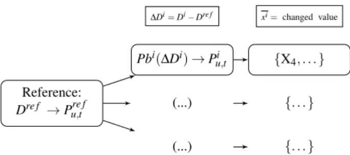
In this section we describe our framework for the nu-merical experiments carried out, including the sources of data and the feature and label engineering for MLC. Reference: Dre f → Pu,tre f (...) (...) Pbi(∆Di) → Pu,ti ∆Di= Di− Dre f {X4, . . . } {. . . } {. . . } xi= changed value
Figure 1: Processing of historical UC data to generate a training dataset.
6.1
Unit Commitment Experiments
we set our reference demand values on a randomly selected calendar day from publicly available demand data1, for the year 2016. The focus is on the variations of the demand D at the 48 time periods of the day, all the other parameters are held fixed. The labels in our MLC problem were the 1632 binary variables of our MILP formulation, letting free the remaining 576 integer variables and 384 real variables.
We then computed the features (∆Dj in Figure 1) as the difference between the reference demand Dre f and perturbations on it. The MLC step yielded the subset XSP of binary labels affected by the random
perturbation, that is, hMLC: ∆D → XSP∈ {0, 1}1632.
XSP are to be let free in the SP resolution, while all
the other binary variables will be blocked to the values found when solving Pre f. To test our meta-algorithm,
we generated 10 perturbed instances on the reference demand. The 10 instances yielded 10 full problems {P}10
i=1. After running the MLC we produce their
rel-ative sub-problems {SP}10i=1.
The 10 instances were solved in their full formula-tion P, using the solvers CPLEX2and the open source Coin-OR CBC3 (Forrest, 2012). We then generated the 10 sub-problems SP associated to each new in-stance and compared the results in terms of relative resolution times and objective values. The results are reported in Table 1.
We observed the SP generation caused a loss of about 2% in terms of objective function, that is, at the end of the minimization the objective value was on av-erage 2.24% greater (i.e. worse) then the true optimal
1
http://www2.nationalgrid.com/uk/Industry- information/Electricity-transmission-operational-data/Data-Explorer/
2IBM ILOG CPLEX Optimizer. Version
12.6.3.0. https://www-01.ibm.com/software/commerce/ optimization/cplex-optimizer/
3CBC MILP Solver. Version: 2.9.7. https://projects.
Table 1: SuSPen on the Unit Commitment problem
Measure Speed-up Objective Loss∗
SPis [×times] faster (SP is worse by [Loss%]) CPLEX† CPLEX‡ CBC†
Min ×1.8 ×2.1 ×3.3 +2.10%
Average ×5.0 ×6.1 ×11.9 +2.24%
Max ×8.3 ×10.7 ×28.7 +2.38%
∗ : CPLEX and CBC converged to the same objective value on all instances. † : Default values for solver.
‡ : Limited pre-solver, no multi-threading, no dynamic search
value. As for resolution times, we observed average speed-ups respectively in the order of ×5 and ×6.1 when using CPLEX with respectively default parame-ters and when “tuned down” to limit its heuristic pow-ers. When running CBC the gains were more relevant, on average twice as much as with CPLEX.
6.2
TSP Experiments
We picked a standard problem (Berlin52) from the TSPLIB4. We selected 10% of nodes at random from the TSP instance berlin52 and perturbed the weights of the nodes within a certain radius ( 50% of the high-est distance between any two nodes) by a factor de-creasing the further apart the nodes are. That is, once a node is picked, the weights within a certain dis-tance are scaled up. If contiguous nodes are selected, then the perturbations will sum up. We produced a dataset of 500 entries, each with comprising the dis-tance matrix and the relative optimal path computed with the Concorde TSP solver. The difference matrix between the reference distance matrix and the new in-stance matrix form the features. For the labels, we started from the reference optimal solution x?re f, taken to be the actual optimum of berlin52. For each entry in the training data, the corresponding optimal TSP path was compared with x?re f, extracting the nodes that were affected by the perturbation. The target predic-tion vectors contains {0, 1}52binary labels, or flags, indicating whether the modifications in the weights of the graph resulted in the optimal solution to change at each node.
For example, if a solution contained: (· · · → 22 → 31 → 35 → 12 → 14 . . . ), but in x?re f we observed:
(· · · → 22 → 31 → 12 → 35 → 14 . . . ), then our binary labels vector will take value “1” for label “12” and “35” and zero for the others.
On average, for the optimal solutions of the per-turbed graphs, 17.2 nodes out of 52 turned out to be
4http://elib.zib.de/pub/mp-testdata/tsp/tsplib/tsp/
Figure 2: Evolution of the objective function over the 200000 iterations (%-completed vs fitness)
affected. On average the predicted label vector should contain 17 non-zero elements, indicating those that deserve the attention of the optimizer and need be re-optimized. After the prediction is obtained, we map these labels back to the x?
re f and find the subsequences
of solution not affected by the perturbations. These subsequences are the “blocked” variables in our SP, that is, the portions of x?re f we assume are still good for our SP. We encode these subsequences as “fake nodes” deleting from the problem the blocked nodes that become invisible to the solver, yielding a problem SPsmaller than the original P.
Figure 2 reports the typical behaviour registered with our approach: solving SP allows us to obtain a good solution rapidly at the cost of some bias (re-lated to the amount of variation in the particular in-stance). In the case of TSP, the underlying assump-tion is that after some perturbaassump-tion is added to a refer-ence instance, the original solution is a good starting point. This is not always the case, and the long-term difference between SP and P can diverge sensibly, as when we block some variables we inevitably intro-duce some error. It would be interesting to further expand this approach by freeing previously blocked variables, allowing SP to continue diving towards a better solution (see the Conclusion for more on this topic).
7
CONCLUSION
This work proposed a meta-algorithm to speed-up the resolution of recurrent combinatorial problems based on available historical data, working under a time bud-get. Although our approach is highly likely to re-sult in sub-optimal solutions, we have shown that it can yield good approximate solutions within a lim-ited time window. It is also interesting both for
exact approaches based on mathematical program-ming (MILP) and approximate stochastic algorithms treated as black-box solvers. Avenues for future re-search includes the extension of our methodology to Mixed Integer Nonlinear Programming (MINLP), where an effective variable selection would possibly grant even more sizeable computational gains. Also of interest is the generalization of the blocking phase to an iterative block/unblock step, thus taking full ad-vantage of the time available for the re-optimization. As seen in Section 6.2, SuSPen allows us to dive deeply towards a good objective value. Being able to unblock some nodes after the initial iterations would likely result in allowing the solution to keep improv-ing, after the initial boost. In case some of the time budgeted for re-optimization is available, instead of limiting us to solve a single SP, one can consider the option of solving more SP’s, eventually in parallel, integrating the information derived from the resolu-tion of previous SP into the learning framework. Fur-thermore, in the case of exact BB-based approaches, we find a natural prospective line of work in the inte-gration of branching rules learned from static frame-works (as seen in Section 2) into our problem-specific approach.
ACKNOWLEDGEMENTS
This research benefited from the support of the “FMJH Program Gaspard Monge in optimization and operation research”, and from the support to this pro-gram from EDF.
REFERENCES
Achterberg, T., Koch, T., and Martin, A. (2005). Branch-ing rules revisited. Operations Research Letters, 33(1):42–54.
Alvarez, A. M., Louveaux, Q., and Wehenkel, L. (2017). A machine learning-based approximation of strong branching. INFORMS Journal on Computing, 29(1):185–195.
Applegate, D., Bixby, R., Chvatal, V., and Cook, W. (2006). Concorde tsp solver.
Applegate, D. L., Bixby, R. E., Chvatal, V., and Cook, W. J. (2011). The traveling salesman problem: a computa-tional study. Princeton university press.
Auger, A. and Doerr, B. (2011). Theory of randomized search heuristics: Foundations and recent develop-ments, volume 1. World Scientific.
Basso, S., Ceselli, A., and Tettamanzi, A. (2017). Random sampling and machine learning to understand good decompositions. Technical Report 2434/487931, Uni-versity of Milan.
Bonami, P., Lodi, A., and Zarpellon, G. (2018). Learning a classification of mixed-integer quadratic program-ming problems. In van Hoeve, W.-J., editor, Inte-gration of Constraint Programming, Artificial Intel-ligence, and Operations Research, pages 595–604, Cham. Springer International Publishing.
Carri´on, M. and Arroyo, J. M. (2006). A computationally efficient mixed-integer linear formulation for the ther-mal unit commitment problem. IEEE Transactions on power systems, 21(3):1371–1378.
Cornelusse, B., Vignal, G., Defourny, B., and Wehenkel, L. (2009). Supervised learning of intra-daily recourse strategies for generation management under uncer-tainties. In PowerTech, 2009 IEEE Bucharest, pages 1–8.
Dai, H., Khalil, E. B., Zhang, Y., Dilkina, B., and Song, L. (2017). Learning combinatorial optimization algo-rithms over graphs. arXiv preprint arXiv:1704.01665. Dantzig, G., Fulkerson, R., and Johnson, S. (1954). So-lution of a large-scale traveling-salesman problem. Journal of the operations research society of America, 2(4):393–410.
Dembczynski, K. J., Cheng, W., and H¨ullermeier, E. (2010). Bayes optimal multilabel classification via probabilis-tic classifier chains. In Proceedings of the 27th In-ternational Conference on Machine Learning (ICML-10), pages 279–286.
Fischetti, M. and Fraccaro, M. (2018). Machine learning meets mathematical optimization to predict the opti-mal production of offshore wind parks. Computers and Operations Research.
Forrest, J. (2012). Cbc (coin-or branch and cut) open-source mixed integer programming solver, 2012. URL https://projects.coin-or.org/Cbc.
Gendreau, M. and Potvin, J.-Y. (2010). Handbook of meta-heuristics, volume 2. Springer.
He, H., Daume III, H., and Eisner, J. M. (2014). Learn-ing to search in branch and bound algorithms. In Advances in Neural Information Processing Systems, pages 3293–3301.
Khalil, E. B., Le Bodic, P., Song, L., Nemhauser, G., and Dilkina, B. (2016). Learning to branch in mixed in-teger programming. In Proceedings of the 30th AAAI Conference on Artificial Intelligence.
Kruber, M., L¨ubbecke, M. E., and Parmentier, A. (2017). Learning when to use a decomposition. In Interna-tional Conference on AI and OR Techniques in Con-straint Programming for Combinatorial Optimization Problems, pages 202–210. Springer.
Larsen, E., Lachapelle, S., Bengio, Y., Frejinger, E., Lacoste-Julien, S., and Lodi, A. (2018). Predicting solution summaries to integer linear programs under imperfect information with machine learning. arXiv preprint arXiv:1807.11876.
Lodi, A. and Zarpellon, G. (2017). On learning and branch-ing: a survey. TOP, pages 1–30.
Loubi`ere, P., Jourdan, A., Siarry, P., and Chelouah, R. (2017). A sensitivity analysis method aimed at en-hancing the metaheuristics for continuous optimiza-tion. Artificial Intelligence Review, pages 1–23.
Mossina, L. and Rachelson, E. (2017). Naive bayes classification for subset selection. arXiv preprint arXiv:1707.06142.
Padhy, N. P. (2004). Unit commitment-a bibliographi-cal survey. IEEE Transactions on power systems, 19(2):1196–1205.
Rachelson, E., Abbes, A. B., and Diemer, S. (2010). Com-bining mixed integer programming and supervised learning for fast re-planning. In 2010 22nd IEEE In-ternational Conference on Tools with Artificial Intel-ligence, volume 2, pages 63–70.
Read, J., Pfahringer, B., Holmes, G., and Frank, E. (2011). Classifier chains for multi-label classification. Ma-chine learning, 85(3):333–359.
Saltelli, A., Ratto, M., Andres, T., Campolongo, F., Cari-boni, J., Gatelli, D., Saisana, M., and Tarantola, S. (2008). Global sensitivity analysis: the primer. John Wiley & Sons.
Schrijver, A. (1998). Theory of linear and integer program-ming. John Wiley & Sons.
Tsoumakas, G. and Vlahavas, I. (2007). Random k-labelsets: an ensemble method for multilabel classi-fication. In European Conference on Machine Learn-ing, pages 406–417. Springer.
Vanderbeck, F. and Wolsey, L. A. (2010). Reformulation and Decomposition of Integer Programs, pages 431– 502. Springer Berlin Heidelberg, Berlin, Heidelberg. Williams, H. P. (2013). Model building in mathematical
programming. John Wiley & Sons.
Zhang, M. L. and Zhou, Z. H. (2014). A review on multi-label learning algorithms. IEEE Transactions on Knowledge and Data Engineering, 26(8):1819– 1837.
Zupaniˇc, D. (1999). Values suggestion in mixed integer pro-gramming by machine learning algorithm. Electronic Notes in discrete Mathematics, 1:74–83.