Insert of sandwich panels sizing through a failure mode map

an author's

https://oatao.univ-toulouse.fr/26730

https://doi.org/10.1016/j.compstruct.2019.111724

Rodríguez Ramírez, Juan de Dios and Castanié, Bruno and Bouvet, Christophe Insert of sandwich panels sizing

through a failure mode map. (2020) Composite Structures, 234. ISSN 0263-8223

investment of time and effort but, in exchange, it could reduce the time and cost of insert design in the long term.

1. Introduction

The aeronautical sandwich structure consists of three main ele-ments: two thin, stiff, strong faces and a thick, light, weak core, often made of Nomex honeycomb. While the faces support the in-plane forces, the core keeps them a certain distance apart, increasing the in-ertia and consequently the bending stiffness, which can be significantly higher than that of heavier laminate sheets. Because of their light weight, these panels are of special interest for aeronautic and aerospace applications[1]and they are used for the main body of helicopters or some business jets like the Beechcraft Starship[2,3]or the Raytheon Premier I. Nevertheless, despite their great advantages, for commercial aircraft, they are restricted to secondary structures such as doors, cabin interiors and control surfaces like ailerons, spoilers, etc. [4,5]. The reason for this is that they are not yet well mastered in terms of man-ufacture, fatigue, damage growth, debonding, assembly, impacts, etc. Sandwich structures are often joined by means of inserts, which are local densifications that raise the core strength, providing the panel with a section where one or many junctions can be installed. This type of assembly is by far the most used for sandwich panels because is simple and, most of the time, handmade, which guarantees low costs. For low load carrying junctions, an insert consists of a metallic threaded fastener that is installed, bonded and sealed into the sandwich panel by injecting adhesive around it; this adhesive is often called potting[6]. 1.1. Overview of analytical approaches for insert sizing

The size and the material of the densified section must be selected to resist the joint loads. There are several methods available to analyze the stress distribution in the vicinity of the insert, which allow a size to be determined for it. The analysis performed by Bozhevolnaya et al. in[7]

or that proposed by Thomsen in[8]. The latter uses the high-order sandwich panel theory (HSAPT) to accurately estimate the stress dis-tribution in the core and skins. The most widely used approach is still the one proposed by the U.S. Forest Product Laboratory in 1953[9], which was adopted by the European Space Agency (ESA) in thefirst insert design handbook or the most recent ECSS-E-HB-32-22A Insert Design Handbook[10]and is also the basis of the modified direct shear approach of Military Handbook 23-A[11]. Finally, the simplest of all is the direct approach by simple shear. Typically, these analytical methods can be implemented quickly.

However, in practice, the pull-out strength estimated by means of the most common analytical approaches often differs from the experi-mental results [12,13]. To better illustrate this, an overview of the accuracy is given inFig. 1. A compilation of several pull-out tests of panels with Nomex honeycomb core performed by several researchers were used as experimental evidence (see Table 5in annex for more details) and the experimental pull-out strengths are compared to the estimations obtained by means of the ESA approach , the military handbook 23-A method and the direct shear approach. The estimations using the ESA method (red bars) are the closest to the experimental results (blue bars), followed by the estimations based on MIL-HBK 23A (which are very similar to those found with the ESA method) and, fi-nally, the least accurate are predicted by the simple shear approach.

Nevertheless, the accuracy of the ESA estimations is very irregular. For some cases the error is between 7.5% and 20% (see comparison of the cases of Heimbs, Kumsantia or Song inFig. 1, for example), which could be considered acceptable; for some others the error is in the ± 50% range, which is considerable (see cases of Roy, Bunyawanichakul or Yong-Bin Park inFig. 1for example). This lack of accuracy of the analytical methods could be explained by the accumulation of errors related to insert manufacturing, the testing procedure and the

https://doi.org/10.1016/j.compstruct.2019.111724

⁎_{Corresponding author.}

analytical calculation method.

From the manufacturing point of view, since inserts are handmade, they are typically full of defects that are not introduced on purpose and which are therefore difficult to predict or quantify.

From the experimental point of view, another source of error might be that there are different methods to identify the insert strength. The most common consist in identifying the end of the linear behavior of the force vs displacement curves, i.e. searching for a change in the slope. In general, a variation of 1%, 2% or 5% is used to detect the end of the linear behavior, and thus, the“structural failure” of the insert[20,23]. Also, there are some references that identify the insert pull-out strength in thefirst peak of the force vs displacement curve[14,15,22,24]. Al-though both approaches are based on the insert stiffness, they identify different points and, thus, different pull-out strengths. Finally, there are few references that identify the insert strength when thefirst compo-nent starts to be damaged or plasticizes[25,26]. According to the re-lated literature, this is mostly the honeycomb core. Yet, identifying the exact moment when a honeycomb structure fails can be a very sub-jective enterprise since, at the beginning of the nonlinear shear beha-vior, it mostly works in a reversible postbuckling regime, and its overall structural behavior could remain elastic even if the cell walls start to plasticize locally as shown in[27]. To state the problem briefly, it is difficult to identify the actual experimental pull-out strength and sub-jectivities inevitably introduce some error.

Finally, from the calculation point of view, another cause could be the actual accuracy of the analytical approaches used to estimate the pull-out strength. This aspect has been addressed by Wolff et al. in[13] where they show that the predicted pull-out strength, calculated using the ESA approach, does not accurately follow the strength trend of the experimental results. This can also be seen in the study by Song et al. [22]. In their research, they evaluated the influence of the variation of the core height, the stacking sequence and skin thickness, and the core density. If the experimental results are compared to the estimations obtained through the ESA approach (seeFig. 2for the variations of core height, skin thicknesses and core density), the shapes of the envelopes of the experimental and the calculated failure loads differ considerably, especially for the skin thickness and core density variations.

Another problem with the accuracy of the analytical method used by ESA is the fact that it relies on several coefficients to include some

considerations, such as the different shear moduli in the W and L di-rections, the maximum and minimum potting size for a given insert diameter, the correction factor of the shear strength depending on the height correction, or even whether a homogenized shear modulus is considered for the core. This aspect is relevant because, if an aspect of the joint is not clear and the coefficients are not chosen correctly, the calculation of the failure load might be wrong (seeFig. 3). Wolff et al. [28]used ESA’s analytical approach for the validation of an insert and presented a very detailed review of the existing coefficients and as-sumptions that can be applied when using this approach. They had to choose between two mathematical formulations for the insert strength, 6 different coefficients to correct the shear strength of the core, 4 homogenization methods for the shear moduli of the core, and 4 dif-ferent models to consider the variations of the potting radius. Even so, they indicated in their conclusions that there was a considerable dif-ference between the final estimation and the experimental pull-out strength. It is also worth mentioning that the inclusion of coefficients in an analytical approach reduces its physical meaning. An example of this can be found in the ESA insert design handbook, which relates the failure of the core under damage in both the W and L directions and states that, due to the percentage of single foils in both directions, an equivalent shear strength should be used instead, which must be cal-culated by multiplying the shear strength of the W direction by a factor of 1.36. The book does not give any more details about how this coefficient is obtained. From our research, reported in[27], we found experimental evidence suggesting that the shear strength of a Nomex honeycomb core can be increased by 16% to 35% depending on the boundary conditions. This happens because the stresses in the cell walls near an insert are better distributed because of the extra stabilization provided by the potting. The authors believe that that it might be very simplistic to reduce such complex phenomena to a simplefixed coef-ficient (the shear strength depends on the coupled postbuckling beha-vior of the Nomex honeycomb structure, so the shear strength changes if defects and/or the boundary change).

1.2. Overview of the numerical approaches for insert sizing

Another approach to estimate the pull-out load of inserts is through F.E. modeling. According to several authors, this approach could

provide a better estimation than the analytical approaches [4,6,17]. This method may offer several serious advantages, since it makes it possible to understand how inserts fail, the order in which the parts start to break and which failures are the most critical. It also allows the influence of some defects to be included and evaluated. Nevertheless, there are some disadvantages: modeling the core and the real potting shape demands considerable expertise and a heavy time investment.

In 2015, this approach was used by Seemann et al. for the virtual testing of inserts[28,29]. First, they focused on the modeling of hon-eycomb cores[30,31]before developing a detailed model of an insert pull-out test. At the end, the results showed consistent agreement with the experimental results and they could reproduce the insert pull-out post-failure behavior, which is quite an achievement considering the complexity of the problem. Nevertheless, it may prove complicated to perform this kind of analysis every time an insert needs to be designed. Also, considering the geometry of the honeycomb cells and all the possible potting shapes, it might be necessary to perform one simulation for each possible potting configuration, which is not practical. All in all, the main limitation of insert sizing through F.E. modeling is the velopment time and the expertise required. A detailed model can de-liver very accurate estimations but the time investment can be high to the point of not being viable. On the other hand, a very rough model might not deliver accurate estimations.

1.3. Insert sizing through virtual testing and failure mode maps

To sum up all these considerations, analytical methods can be ra-pidly implemented but the accuracy of the predictions could be ques-tionable, and they also rely on the correct choice of coefficients. In contrast, the development of F.E. models may give more accurate es-timations but the expertise required and the time invested are not very encouraging. From a practical point of view, both methods present several advantages and disadvantages. For example, the ESA method implements a statistical approach to consider the different potting shapes within an equivalent minimal, typical or maximal value of the potting radius, which allows the number of calculations to be reduced. For the F.E. approach, the main advantage is the accuracy of the pre-dictions.

In the present research, the advantages of both methods are com-bined to draw a failure mode map of inserts subjected to pull-out loading. The idea is to use these failure maps as tool for the rapid sizing of inserts. First, an F.E. model of an insert pull-out test is developed and validated through experimental tests. This model is not as detailed as the models developed by Roy et al. in[20], Seeman et al. in[14,31]or Slimane et al. in[32]. Instead, several simplifications proposed by ESA in[10]and the ideas and results presented previously in[27,33]are considered. These simplifications reduce the development and

Fig. 2. Comparison of the experimental and calculated pull-out strengths of the pull-out tests performed by Song et al.[22]. The ESA and the experimental tests have

different tendencies.

calculation time. Then, this model is parametrized by means of Abaqus and Python scripting in order to be used intensively to draw an example of a failure mode map for inserts.

2. Development of the insert numerical model for virtual testing This section presents the main aspects of the numerical modeling of insert pull-out tests. It is well known that numerical models are often used for the design of structures. They give a consistent estimation of the strains and stresses, which is very useful for the embodiment design stage. These models are known to reliably predict the linear behavior of structures. However, when nonlinear considerations are included, such as contact, buckling or material degradations, their predictions cannot be accurate unless great care is taken when introducing such aspects. For this reason, the numerical analysis using nonlinear models must be always validated through experimental tests. The role of the experiment is to allow key information be collected that can be used as guide for the development of the nonlinear model. In this sense, once the numerical model is capable of reproducing the nonlinear behavior of the structure, its role is to provide insight into the analysis of stresses and deforma-tions that cannot be measured experimentally. This numerical-experi-mental dialogue is very helpful to better understand how and why structures fail. For this reason, the development of the insert numerical model that follows is divided into several steps. First, several pull-out tests are performed to gather the experimental evidence needed. Then, the development of the numerical model of the insert is presented to correlate with the experimental linear behavior of the experiments. 2.1. Gathering the experimental evidence: insert pull-out testing

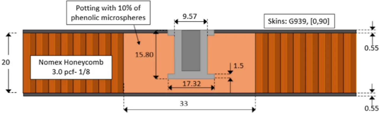
Seven insert pull-out tests were performed to gather the experi-mental evidence needed for the numerical model. The specimens cor-responded to the specifications of sandwich panels used for helicopter interiors. The material properties are shown inTable 1. The skins are made of two layers of G939/145, the core is in Nomex honeycomb, and the insert is potted with Araldite AV121B mixed with 10% of its weight of phenolic microspheres with an average diameter of 90 µm. These specimens were left over from a series manufactured for the research presented in[21]. All of them were made using the material and geo-metry specifications shown inFig. 4. First, a hole 17.32 mm in diameter was made in the panel and an undercut was performed to increase the diameter of the insert potted section to 33 mm. Finally, the metal insert was placed, and the potting was injected. The specimens were left to cure at room temperature for several days.

2.1.1. Test setup

To perform the tests, a testfixture was used as recommended by ESA in[10]. The center hole had a diameter of 60 mm and a 10 kN Instron machine was employed. The displacement was imposed at a constant speed of 0.5 mm/min. The applied force was measured directly from the machine while a 3D digital image correlation system was used for the displacement. This setup measured the actual pull-out displacement applied to the insert, which was defined as the difference between the metal insert displacement and the skin touching the borders of the test fixture as shown inFig. 5. Two LDVT sensors were used to measure the imposed displacement but the data obtained were not coherent. 2.1.2. Test results and analysis

The test curves are shown inFig. 6b. The average linear stiffness of the specimens was 6750 N/mm, and the average failure load according to the 5% failure criterion was 1091 N, while the maximum and minimum failure loads were 1281 N and 857 N respectively. These failure loads were calculated by inspecting the stiffness of the tested specimens (omitting the initial contact effects) and then searching for a change equal to or greater than 5% in the stiffness (see Fig. 6a). A MATLAB script was developed to avoid detections of local changes Table

1 Properties of the materials of the sandwich panel and the insert. Part/Material E1 [MPa] E2 [MPa] E3 [MPa] υ12 υ21 υ21 G12 [MPa] G13 [MPa] G23 [MPa] σ1 [MPa] σ2 [MPa] σ3 [MPa] τ12 [MPa] τ13 [MPa] τ13 [MPa] Skins G939/145.8 50,500 50,500 5000 0.02 0.29 0.29 32,000 3500 3500 634 634 – 100 80 80 Honeycomb core 3.0 pcf − 1/8 in 1 1 94 0.29 0.02 0.02 1 17 26 –– 7.5 – 0.3 0.48 Potting 10% of phenolic micro-spheres 1312 0.3 504 504 504 35 35 35 –– – Stainless steel Insert 210,000 0.3 80,800 –––– – –

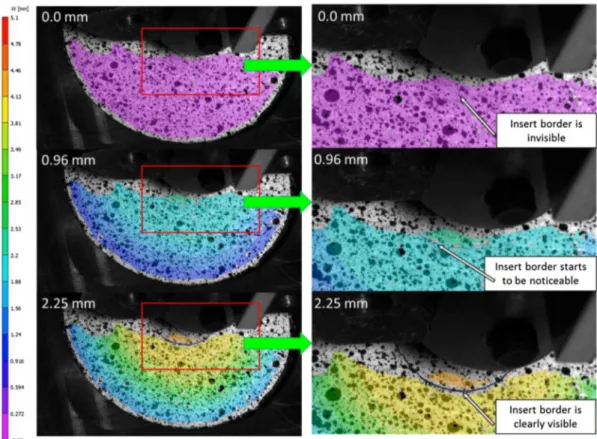
(fake failures) due to noise in the force and displacement signals. During the test, the detaching of the metal insert from the skins (see Fig. 7) could be observed with the naked eye. For EP1, this started to be noticeable at 0.96 mm of displacement.

Then, the tested specimens were cut in half to be inspected. Several remarks can be made. The potting diameter was supposed to be 33 mm but, in the specimens, it varied from 30 mm to 39 mm - as expected due to the discrete nature of the honeycomb cells. At first sight, all the fasteners were well bonded since none of them became detached from the potting. Also, the breaking of the potting surrounding the insert (as the images shown inFig. 7may suggest) only appeared for two speci-mens (EP5 and EP7) and not for the others. This may have been because the small fractures or gaps closed when the pull-out load was removed. As expected for inserts installed by hand, there were many air bubbles and the borders of the potting were very irregular. Several failure modes can be identified: core shear failure (buckling and collapse of the cells), tensile breaking of the core, fracture of the potting, and breaking of the potting/skin interface (seeFig. 8).

The folding of the honeycomb cells appeared to start from the upper three-material contact point (potting, skin, honeycomb) for both double or single walls as can be seen in the sections of EP1, EP3, EP5 or EP6 shown inFig. 8. This seems contradictory to the concept of effective potting radius explained by ESA in[10], which states that the double walls next to the potting do not fold and, thus, the failure should appear only in the nearest single walls. Concerning the estimation of the pull-out strength using the ESA approach, with an effective potting radius of 19.04 mm, using a factor of 1.36 for the correction of the core shear strength as suggested in[10](which results in an admissible shear of 0.41 MPa for the honeycomb core) and a homogenized shear modulus of the core of 21.5 MPa, the failure load should be around 1363 N. This estimation is out of the range of the maximum and minimum strengths measured experimentally (see red dashed lines in Fig. 6b) and over-estimates the average failure load (detected by the 5% dev. criterion) by 24% (see dashed blue line inFig. 6b).

Fig. 4. General description of the insert specimens tested.

2.2. Numerical modeling of the insert

In this sense, the pull-out tests are intended to be reproduced nu-merically. To do this, the properties and geometry given inTable 1and Fig. 4are considered and, since the testing speed was very low, the insert was modeled using Abaqus implicit. In contrast to the very de-tailed models of Seemann[29], Roy[20]or Slimane[32], the numer-ical model of this research is kept as simple as possible to reduce the calculation time, bearing in mind that the accuracy should not be compromised too much. For this reason, whenever possible, the geo-metry of the specimens is simplified to facilitate its parameterization and a homogenized continuum 3D approach is used to represent the

materials. The potting geometry is drawn as a regular cylinder of radius 18.43 mm regardless of the irregular shape it typically has due to the discrete nature of the honeycomb cells (seeFig. 7). This simplification is based on the Real Potting Radius (RPR) also proposed by ESA in[10], which is congruent with the evidence ofFig. 8, where both single and double walls fold without distinction. It is important not to confuse the Real Potting Radius and the Effective Potting Radius (EPR). The first is calculated considering an equivalent potted circular surface, while the EPR is calculated considering that only the single walls fail. For clarity, this distinction is illustrated inFig. 9.

Also, the fastener geometry was simplified as shown inFig. 10-a. The original contact surface areas between the metallic insert and the

Fig. 6. a) Example of the calculation of the failure load of the inserts according to the 5% deviation criterion, b) Experimental curves of the pull-out tests.

potting were replaced by a simplified equivalent surface. As explained in[27], the honeycomb cells that surround the insert might have dif-ferent shear behaviors. Briefly, this is because the potting creates a lateral stabilization effect that alters the shear behavior of the sur-rounding cells. For this reason, the core is divided into two sections: one near the insert (Fig. 10b in blue) with a radius of two cells beyond the

potting, and the other the rest of the honeycomb (in red). As for the types of elements, only brick elements are used to represent the mate-rials, including the skins, the honeycomb core, the potting and the fastener. For the core, this allowed the CDM approach presented in[33] to be implemented, providing a good alternative to include the shear nonlinear behavior of the core at low computational cost.

2.2.1. Material laws

The elastic material properties given in Table 1 are considered. However, to detect the insert pull-out strength, material failures are included in the numerical model through behavior laws (UMAT for Abaqus standard) for the CFRP skins, the potting, and the Nomex honeycomb core (seeFig. 11). For the skins, the in-plane and trans-versal matrix failure are included at 100 MPa and 80 MPa respectively. After these limits, the stiffnesses in the respective directions are reduced by 85% to avoid numerical instabilities and they are not coupled (see Fig. 11a). This value is sufficient, since the objective is to follow only the beginning of the nonlinear behavior here. The behavior of the potting under tension includes a Young modulus of 1660 MPa and brittle fracture at 14.5 MPa. After this limit, the stiffness is reduced by 99% to simulate a brittle failure. On the other hand, under compression, the Young modulus of the material is 1226 MPa and the behavior law includes an isotropic perfect plasticity model starting at 26 MPa. The

Fig. 8. Identification of the failure modes of the tested specimens.

Fig. 9. Real potting radius (green surface) vs Effective potting radius (red

da-shed line), reproduced from[10].

shear failure of the potting material is not included (see Fig. 11-b). Finally, for the Nomex honeycomb core, the CDM approach presented in [33]is implemented. This method uses two different variables to consider,first, the effect of the elastic reversible buckling of the cells and, second, the permanent damage of the collapsing cells. This ap-proach is used to simulate the shear nonlinear behavior of the cells near and far from the insert. The coefficients ofTable 2refer to the approach presented in[33]. The nonlinear behavior of cells starts atγ_b0and they collapse at γ_c0. The resulting behavior laws are shown inFig. 11c.

2.2.2. Meshing and boundary conditions

For the meshing, the skins are composed of two layers and therefore they have two elements of thickness each. The core is meshed with only one element as explained in[33]and, for the rest of the parts, the size can vary according to the accuracy desired. Symmetry is considered and only one quarter of the specimen is modeled. Also, the Z displacement of the upper skin nodes at a radius of 30 mm is restricted to include the effect of the testing support (seeFig. 5). The displacement is imposed at the center of the fastener as shown inFig. 12

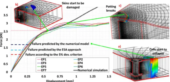
2.2.3. Validation of the numerical model: real test vs numerical testing The numerical simulation was performed using 8 processors and 8 GB of RAM. The calculation took 7 min. The numerical curves showed good correlation with the experimental results up to a displacement of 0.85 mm. The core shear failure was well represented, and the cells were seen to start to collapse a few millimeters away from the potting (seeFig. 13-a) as the analytical approach in[10]suggests. Breaking of the potting appeared in the upper borders surrounding the insert (see Fig. 13) after 0.9 mm of imposed displacement, which is consistent with the experimental evidence shown in Fig. 7. As for the skin matrix failure, the numerical model suggests it appears before the potting

breaks but, unfortunately it was not possible to verify this experimen-tally.

The lower potting/skin interface does not appear since the breaking of the potting/ skin interface was not included in the model. This could explain the difference of the numerical and experimental curves after 0.85 mm of displacement. Also, the breaking of the potting beneath the insert that appeared in specimens EP3 and EP5 (letter d inFig. 8) does not show up. Both of the last failures modes may be related to the in-clusion of defects; the lower skins were not properly degreased and cleaned before the injection of the potting so the interface might have been very weak and easy to break. As far as the breaking of the potting is concerned, it could be explained by a higher local concentration of phenolic microspheres or an inefficient degreasing of the bottom of the metal insert, which would have weakened the potting or the potting-insert interface in the zone where the fracture appears in the real tests. It is also worth mentioning that the numerical model predicts a max-imum stress of about 9 MPa beneath the insert, which is lower than the tensile elastic limit of the behavior law, of 14.5 MPa.

2.2.4. Conclusions on the numerical approach for virtual testing of inserts Setting aside the problems mentioned above, this simplified nu-merical approach can detect the activation of three failure modes:first the shear collapse of the cell walls of the core at 0.34 mm of dis-placement, followed by the in-plane matrix failure of the skins at 0.7 mm of displacement, and then the potting breaking in the upper borders next to the metal insert. The fact that the core shear failure appears before any other failure is consistent with the typical failure of most inserts, as ESA states in[10]. Nevertheless, the numerical model predicts core shear failure at 1750 N while the analytical approach of ESA estimates the failure at 1363N and, experimentally, according to the 5% dev. criterion, the failure load is 1091N.

Fig. 11. a) Shear behavior laws of the skins, b) traction-compression behavior laws of the potting and c) shear behavior laws of the honeycomb core.

Table 2

Parameters used for the behavior laws of the honeycomb core in the CDM

ap-proach presented in[33]. W dir. (near the insert) L dir. (near the insert) W dir. (far from the insert) L dir. (far om the insert) Initial buckling stage Ab 0.9 0.9 0.9 0.9 λb 0.057 0.05 0.057 0.05 γb0 0.015 0.19 0.015 0.19 kb 1.35 1.35 1.35 1.35 Collapse stage Ac 0.5 0.5 0.36 0.34 λc 0.015 0.015 0.025 0.025 γc0 0.03 0.018 0.03 0.03 kc 2 2 1.5 1.5

It should not be forgotten that the 5% dev criterion is not based on the integrity of the sandwich and insert materials but on the overall insert behavior, and this could be very penalizing for sandwich panel inserts with a Nomex honeycomb core. The research presented in[27], where it is shown that Nomex honeycomb core exhibits reversible elastic buckling under shear loads and, more importantly, that most of the shear behavior happens to be in this nonlinear elastic behavior zone, suggests that using a criterion based on the linear behavior (such as the 5% dev. criterion) penalizes and underestimates the actual strength of the insert. Even so, this criterion is largely used for insert testing as it is practical and estimates the failure load with a certain safety margin (see for example[20,26]). For these cases, it could be more profitable to identify the true shear stress at which the core starts to be damaged (or the point where the cells start to collapse) and to implement this limit in a numerical model, as was done for this research (except that the admissible shear stress used here was assumed and not identified experimentally).

In conclusion, the simplified numerical modeling presented in this research has several advantages. It allows the most common failure modes, such as core, potting and skin matrix failure, to be detected. It also allows the nonlinear elastic behavior of the honeycomb core to be taken into consideration (which cannot be done analytically) and, thanks to the CDM approach used for the honeycomb core[33], the simulation time was about 7 min, which is very important since a parametric study is foreseen. Also, this numerical model is useful to understand how the insert fails and the order in which the materials do so. When the pullout load is applied, the core is subjected to shear stress. Then, thefirst change of slope in the insert behavior is caused by the buckling of the honeycomb core, which reaches a bifurcation point. Then, matrix failure is detected. The potting apparently breaks in the upper borders touching the metal insert. It should be noted that, as far as the potting breaking prediction is concerned, this is only a rough analysis since the failure of syntactic polymer foams is much more complex. A more detailed study, possibly including fatigue, could result in the prediction of the potting breaking even earlier than the core shear failure, which could help to explain the issues related to the water sealing joints of sandwich panels presented by Shafizadeh et al. in[5].

3. Plotting the insert failure mode map 3.1. Introduction

Failure mode maps describe the different failure modes of a

structure in terms of its intrinsic properties like dimensions, materials, boundary conditions, etc. An example of this was presented by Triantafillou et al. in[34]or by Petras et al. in[35], where the different failures of the sandwich structure are represented using a map. Petras compiled the formulas used to calculate the various strengths of the failure modes of sandwich panels under certain conditions, like face yielding, face wrinkling, and core shear failure, among others. Then, all these expressions were evaluated to determine which failure mode was activated first. At the end, they obtained a chart where the failure modes could be easily identified according to the properties of the sandwich. This same approach has been proposed by other authors like Vitale et al.[36]to tackle complex problems for the description of the failure of natural and synthetic fiber reinforced composite sandwich panels, or Andrews et al.[37]to represent the failure modes of com-posite sandwich panels subjected to air blast loading.

The creation of failure mode maps enables the transition limits of different failure modes to be detected, which are of special interest for mass reduction problems because they point out the structural para-meters that present the best compromise between strength and mass. This is interesting for aeronautical structures but such optimization might be difficult for complex structures that rely on several para-meters. This is the case of inserts for sandwich panels. As quick ex-ample, let us consider that, if the core is always thefirst component to fail, atfirst sight there is no sense in using a stronger potting adhesive or a metallic insert that might add unnecessary weight to the panel; a lighter insert and potting could help to save a few kilograms, given the total number of inserts in a structure. For this reason, a failure mode map of inserts could help to reduce the weight of structures Nevertheless, there are many different types of sandwich configurations and choices are made according to needs. For this reason, it could be very complex to create a general failure mode map of inserts since their strength relies on the several dimensions and the materials that can be used.

It is important to emphasize that this research only proposes a path that could be followed to draw an insert failure mode map, which should be used only for the design of similar types of inserts, e.g., in the case studied here, fully potted inserts for aeronautical sandwiches with thin CFRP skins and a 20 mm thick Nomex honeycomb core. Also, this failure mode map does not consider the influence of defects and the mechanical properties of the potting used for the parametrical study are not the same as those used for the numerical model in the previous section. This is because, in the literature (seeTable 5in annex) most inserts are potted with pure adhesive and not with syntactic polymer

foam like the specimens presented in the previous section. Therefore, the failure mode map that will be presented is only provided for de-monstration purposes.

3.2. Parametric study of the insert pull-out strength

The next step of this research is to use the previously presented, simplified numerical approach to the insert in order to perform a parametric study and plot the insert failure mode maps. To do this, the numerical model was parameterized using Python and Abaqus scripting. Each move made on the CAE environment was recorded using the macro editor. In this way, Abaqus wrote the code necessary to build the numerical model, which could then be modified by the user ac-cording to the needs. This was of practical advantage because it was not necessary for the user to have a solid background in Abaqus scripting

commands. The size of the sandwich specimen was fixed at

100 × 100 mm (actually 50 mm because only a quarter of the model was simulated) with a core thickness of 20 mm. Also, the support radius

was fixed at 30 mm and the model geometry and mesh size were

parameterized accordingly.

Concerning the sandwich panel, the same honeycomb core as used for the specimens presented in last section was considered, with a cell size of 1/8 in., 20 mm thickness and a density of 48 kg/m3. For the skins, the same G0939/145.8 CFRP woven fabric was used. Also, to make the simulations easy to track, the script was modified to perform and arrange the simulations in different directories. In this way, the simulations were numbered, stored and described automatically. For the metal insert, a smaller type was used. Finally, only 1 mm of dis-placement was imposed for the virtual tests. There are several para-meters that can be chosen to plot failure mode maps. For this research, the authors chose the RPR, the tensile strength of the potting and the skin thickness. The RPR was swept from 9.5 mm to 23.5 mm since most of inserts of the literature are in this range (see Table 5). The me-chanical properties of the potting varied according to the values shown inTable 4. The number of skin layers was swept from 1 to 4, which is equivalent to sweeping from 0.275 mm to 1.1 mm of thickness. Each layer was stacked following a [0°, 90°] orientation with respect to the preceding one.

3.2.1. Sweep of the real potting radius

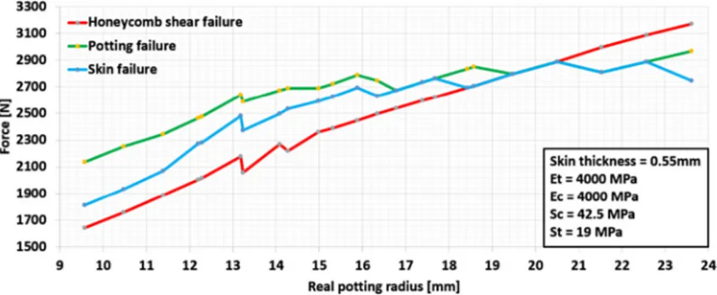
The properties of the materials that were used for the parametric study of the potting radius are shown inTable 3. A total of 23 simu-lations were performed. The failure loads of each component were identified, and the results are shown inFig. 14. Thefirst remark is the presence of small variations (like noise) in the curves. This is was caused by the discrete time increments of the simulations, which were set automatically by the software. However, the general trend of the curves is clear.

Note that, between 9.5 mm and 18.5 mm of RPR, it is the core shear failure that occursfirst. This is coincident with the observations of ESA in[10]and most researchers[18,25]that have performed pull-out tests with inserts in this range of RPR radius.

Then, for the interval between 18.5 mm and 20.5 mm, the three parts failed almost simultaneously while, for an RPR bigger than 20.5 mm to 22.5 mm, the potting and skins failed before the core and, finally, when the radius was greater than 22.5 mm, the skins failed before all the other parts. This shows that, for a relatively large RPR, the triple failure scenario is possible. However, in practice, the skin matrix failure can only be detected by looking the specimen skins under the microscope or by thermography, and it might escape the sight of re-searchers because the other failures are much more visible. Moreover, it can be appreciated that there is almost a linear relation between the insert strength and the RPR real potting radius.

3.2.2. Sweep of the potting properties

For this part of the parametric study, the RPR wasfixed at 9.5 mm, and the potting properties were swept according to the values shown in Table 4. The initial value corresponded to the actual properties of Araldite AV-121B, the rest of the properties were the interpolation values between the original properties and these properties divided by four. This was done for the elastic modulus, the tensile strength and the compressive strength. A total of 13 simulations were performed and the results are shown inFig. 15.

It is important to emphasize that, in the results chart ofFig. 15, the potting sweep is only represented by the potting tensile strength be-cause it is the most influential parameter for insert failure. Never-theless, all the other parameters were swept according toTable 4. Ac-cording to these results, the insert failure was caused mostly by core shear failure. Therefore, the insert strength remained constant until the potting became weak enough and failedfirst.

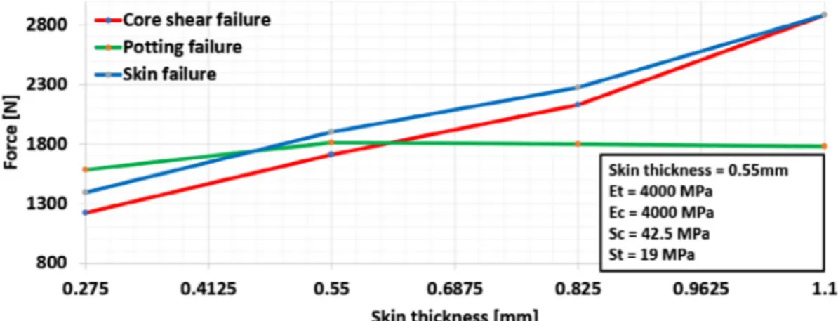
3.2.3. Sweep of the skin thickness

As in the previous studies, the insert parameters werefixed, except for the thickness of the skins, which was swept from 1 to 4 layers for a total thickness of 0.275 mm, 0.55 mm, 0.825 mm, or 1.1 mm. Four simulations were performed, and the results are shown inFig. 16. Also, it is important to emphasize that the skins had the same number of elements in the thickness as layers, except for one layer where two elements were used. The same mechanical properties of the prepreg were used for all the thicknesses. This might be debatable because, when a prepreg is stacked, the mechanical properties are reduced due to porosities and voids among other defects that can be introduced. However, these effects were neglected to simplify the study.

The results show that there was a failure transition when 3 layers were used for the skins. When the skins were thin, thefirst failure was core shear failure while, when the skins were thick, the predominant failure was potting failure. This happened because, when the skins are thin, the core can be easily deformed in shear and thus absorb the load, while for thick skins, the skins become stiffer and absorb the shear loads, thus protecting the core.

3.3. Failure mode map

The failure mode maps of inserts can be plotted by sweeping two

Table 3

Values used for the parametric study of inserts.

Skins

Reference e [mm] E [MPa] v t12 max [MPa] t13 max [MPa] t23 max [MPa]

G0939/145.8 [0/90] 0.275 to 1.1 52,000 0.09 100 80 80

Core

Reference C [mm] G_W [MPa] G_L [MPa] t_adm W [MPa] t_adm L [MPa] Density [pcf]

Nomex® phenolic 20 17 26 0.26 0.45 3

Insert

Reference Real potting radius [mm] E [MPa] v St max [MPa] Sc max [MPa] Support radius [mm]

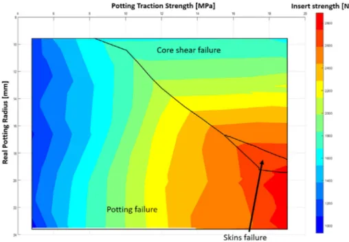
design parameters at the same time, although, for this research, only one combination is presented in the following section. A total of 60 simulations were run and each calculation took around 5 min to com-plete. For every simulation the three failure modes were identified, and the load corresponding to each failure mode was used to draw three different surfaces, i.e. each surface was composed of 60 points, as shown inFig. 17. Although more points could have been obtained, this was considered enough to study the tendency of the failure modes. Insert failure should be produced by the lowest load value of the three failure modes and this is equivalent to viewing the surfaces from the bottom, which is shown inFig. 18. Notice that, most of the time, it was the core or the potting that failed, and only a small area was composed by the skin failure.

As for the interpretation of the failure mode map; when the insert radius is increased, the potting failure is predominant. This is logical since the contact area between the potting and the fastener remains the same, while the section of the honeycomb core subjected to shear in-creases (therefore the shear stress concentration dein-creases). Also, as the tensile resistance of the potting increases, the core shear failure be-comes predominant. This occurs because the potting bebe-comes stronger, and can withstand higher loads, while the honeycomb core has the same resistance. When both variables are increased at the same time, there is a transition between the potting failure and the core shear

failure, until the applied load is high enough to start to damage the skins before the core and the potting.

Also, in order to show the insert strength as well as the failure modes, a color scale can be used to represent the load range of the insert strength. This is shown inFig. 19.It can be seen that the insert strength increases as the design parameters do. The color map shows there are different insert configurations that provide similar strength. An ex-ample of a criterion for choosing one combination of parameters could be the mass, in which case the configuration with the lowest mass should be used. This type of tool could be very useful for design pur-poses since it compacts a huge quantity of information into a single 2D chart that can be easily shared among designers.

4. General conclusions

The most common analytical approaches provide a rough estima-tion of the pull-out strength of inserts and their accuracy relies on the correct selection of coefficients for the correction of the parameters. The failure of inserts can also be measured experimentally but the exact failure point is hard to identify since it is not possible to observe the integrity of the components in real time during the test. Moreover, testing is expensive and could take a considerable amount of time. In this context, the virtual testing of inserts proves to be an advantageous

Fig. 14. Failure of the skins, potting and honeycomb core; insert failure load vs Real Potting Radius.

Fig. 15. Failure of the skins, potting and honeycomb core; insert failure load vs tensile resistance of potting.

Table 4

Sweeping values for the adhesive based on Araldite AV-121B.

Original properties Sweep values Properties/4

Tensile Strength [MPa] 19 17.81 16.6 15.4 14.3 13.1 11.9 10.7 9.5 8.3 7.1 6.0 4.8

Compression Strength [MPa] 42.5 39.8 37.2 34.5 31.9 29.2 26.6 23.9 21.3 18.6 16.0 13.3 10.6

Elastic Modulus [MPa] 4000 3750 3500 3250 3000 2750 2500 2250 2000 1750 1500 1250 1000

Table 5 Characteristics of several pull-out tests of inserts in sandwich panels with Nomex honeycomb core [14 –21] . Skins Core Insert Test Reference Thickness [mm] E [MPa] Poisson ratio Reference Height [mm] Height correction factor

G13 W [MPa] G23 L [MPa] t_adm13 [MPa] t_adm23 [MPa] Reference Support radius [mm] Insert radius [mm] Eff . Pot. radius [mm] Failure load [kN] Failure criterion Through-thickness insert (Song 2008) P01 wsn3k SK chemical [45,0]s 0.84 49,108 0.34 Nomex ® PN2-3.0 –1/8 17.78 0.96 24 46 0.69 1.35 Hysol EA9394 30 7.5 10.04 1890 First peak Through-thickness insert (Song 2008) P02 wsn3k SK chemical [45,0]s 0.84 49,108 0.34 Nomex ® PN2-3.0 –1/8 22.86 0.90 24 46 0.65 1.27 Hysol EA9394 30 7.5 10.04 2320 First peak Through-thickness insert (Song 2008) P03 wsn3k SK chemical [45,0]s 0.84 49,108 0.34 Nomex ® PN2-3.0 –1/8 27.94 0.85 24 46 0.61 1.20 Hysol EA9394 30 7.5 10.04 2640 First peak Through-thickness insert (Song 2008) P04 wsn3k SK chemical [45,0]s 0.84 49,108 0.34 Nomex ® PN2-5.0 –1/8 17.78 0.96 42 74 1.42 2.14 Hysol EA9394 30 7.5 10.04 2740 First peak Through-thickness insert (Song 2008) P05 wsn3k SK chemical [45,0]s 0.84 49,108 0.34 Nomex ® PN2-8.0 –1/8 17.78 0.96 73 115 1.94 2.78 Hysol EA9394 30 7.5 10.04 4480 First peak Through-thickness insert (Song 2008) P06 wsn3k SK chemical [45,0,45]s 1.26 39,437 0.47 Nomex ® PN2-3.0 –1/8 17.78 0.96 24 46 0.69 1.35 Hysol EA9394 30 7.5 10.04 2620 First peak Through-thickness insert (Song 2008) P07 wsn3k SK chemical [45,0]2s 1.68 49,108 0.34 Nomex ® PN2-3.0 –1/8 17.78 0.96 24 46 0.69 1.35 Hysol EA9394 30 7.5 10.04 3170 First peak Through-thickness insert (Song 2008) P08 wsn3k SK chemical [45,0]s 0.84 49,108 0.34 Nomex ® PN2-3.0 –1/8 17.78 0.96 24 46 0.69 1.35 Hysol EA9394 30 7.5 10.04 1840 First peak Blind full potting insert (Kumsantia 2010) G0939/ 145.8 [0/ 90] 0.55 52,000 0.09 Nomex ® honeycomb 3.0 pcf − 1/8 20 0.93 17 26 0.30 0.45

EA9396 STRUCTIL −10%mb phenol

30 16.5 19.04 1200 Aprox. Through-thickness insert (Roy 2013) 2-ply Cytec G30-500 –3k -PW/5276 –1 [0,45] 0.2 49,044 0.36 Nomex ® HRH-10 –1/8 –3.0 13 1.02 24.13 44.81 0.70 1.23 Magnobnd 6398 40 10.5 13.04 859 2% dev Through-thickness insert (Roy 2013) 3-ply Cytec G30-500 –3k -PW/5276 –1 [0,45,0] 0.3 56,669 0.26 Nomex ® HRH-10 –1/8 –3.0 13 1.02 24.13 44.81 0.70 1.23 Magnobnd 6398 40 10.5 13.04 893 2% dev Through the thickness insert (Raghu 2009) 2 plies 7781 E-glass/ phenolic 0.508 2176 0.3 Nomex ® HRH-10 –1/8 –3.0 25.4 0.88 24.13 44.81 0.60 1.05 3 M EC-2216B/A Epoxy 40 10 12.54 1353 Estimated Blind full potting insert (Raghu 2009) 2 plies 7781 E-glass/ phenolic 0.508 2176 0.3 Nomex ® HRH-10 –1/8 –3.0 25.4 0.88 24.13 44.81 0.60 1.05 3 M EC-2216B/A Epoxy 40 10 12.54 1285.35 Estimated Blind partial potting insert (Raghu 2009) 2 plies 7781 E-glass/ phenolic 0.508 2176 0.3 Nomex ® HRH-10 –1/8 –3.0 25.4 0.88 24.13 44.81 0.60 1.05 3 M EC-2216B/A Epozy 40 10 12.54 1082.4 Estimated Blind full potting insert type 1 (Bunyawanichakul 2005) G0939/ 145.8 [0/ 90] 0.55 52,000 0.09 Nomex ® honeycomb 3.0 pcf − 1/8 20 0.93 17 26 0.30 0.51 AV-121B- 10%mb phenol 30 9 11.54 1465 1% linear regression (continued on next page )

Table 5 (continued ) Skins Core Insert Reference Thickness [mm] E [MPa] Poisson ratio Reference Height [mm] Height correction factor

G13 W [MPa] G23 L [MPa] t_adm13 [MPa] t_adm23 [MPa] Reference Support radius [mm] Insert radius [mm] Blind full potting insert type 2 (Bunyawanichakul 2005) G0939/ 145.8 [0/ 90] 0.55 52,000 0.09 Nomex ® honeycomb 3.0 pcf − 1/8 20 0.93 17 26 0.30 0.51 AV-121B- 10%mb phenol 30 18 Blind full potting insert type 3 (Bunyawanichakul 2005) G0939/ 145.8 [0/ 90] 0.55 52,000 0.09 Nomex honeycomb 3.0 pcf − 1/8 20 0.93 17 26 0.30 0.51 AV-121B- 10%mb phenol 30 9 Through-thickness insert (Bunyawanichakul 2005) G803/914 [0,45,]8s 2.6 41,810 0.29 Nomex ® honeycomb 3.0 pcf-3/16 20 0.93 24.13 31.71 0.51 0.80 3 M 3500-2B/A 30 7.5 Full potting insert (Heimbs and Pein 2009)

E-glass/ phenolic Stesalit PHG 600

–68-50 0.24 20,000 0.059 Nomex ® Schütz Cormaster C1-3.2 –48 − 1/8 14.6 1.00 25.5 41.9 1.21 0.80 Cytec BR 632 B4/ Huntsman Araldite 2011 50 19 Blind full potting insert (Yong-Bin Park 2014) Cytec 5250 –4/ T650-35 3K70PW [45,0,45] 0.654 47,094 0.4 Nomex ® Gilcore HD322 2.0 pcf − 3/16 25.4 0.88 11.7 20 0.27 0.48 Magnobnd 6398 40 10 Blind partial potting insert (Seemann 2018) cabin interior ABS 5047 –07 00.25 22,350 0.15 Nomex honeycomb 3.0 pcf − 1/8 26 0.87 20 36 0.72 1.32 Epoxy 40 7

technique to reduce time and costs while providing accurate estima-tions. Nevertheless, the development of a detailed numerical model can take several months, depending on the problem. For this reason, in this research, a simplified numerical model is proposed to plot a failure mode map, which could be an innovative tool to speed up insert sizing. Thefirst step was to gather the experimental evidence needed for the development of the simplified numerical model. The pull-out tests performed provided solid evidence of the most common damage that can be found for these types of inserts; core shear failure and potting failure as well as the detachment of the potting from the lower skin. Also, it is important to mention that the use of LVDT sensors provided incoherent values for the displacement, while the use of a 3D DIC system was useful to capture the actual displacement applied to the insert. There is evidence suggesting the detaching of the metal insert from the sandwich panel as shown inFig. 7.

In addition, the experimental evidence suggests that the hypothesis of the RPR is more suitable than the EPR to describe the insert size. This could be the case at least for Nomex honeycomb sandwich panels. The simplified numerical modeling was shown to be useful to detect core shear failure, potting failure and skin failure, in an accurate way and at very low computational cost. Also, this numerical approach allows the

nonlinear elastic behavior of the Nomex honeycomb core to be in-cluded, by using the approach presented in[32], which is not possible in analytical models. It should be recalled that the skin failure predicted by the numerical model can pass unperceived and it could be im-portant.

The failure mode maps permit the strength of an insert to be ob-served in a very easy way as a function of the principal design variables, i.e. the size of the potting and the potting material. This tool should be very useful for engineers since it compresses the very accurate results based on F.E. simulations into a simple 2D chart. Also, it has been shown that this failure mode map can be helpful in selecting the best combination of parameters to obtain the best mass to strength ratio. This is easy to see inFig. 19. The best insert design is the one with the lowest radius and with a potting material selected to resist the required pull-out strength.

Acknowledgments

The present work was supported in part by the CONACYT from Mexico through the program“Becas Conacyt- Gobierno Frances”, the “Institut Clement Ader” and INSA Toulouse. This support is

Fig. 16. Failure modes vs thickness of the skins.

acknowledged with thanks. The authors are also grateful to Benoît Porra of IMT Mines Albi, and to Matheus Pessanha and Thomas Salomon from INSA Toulouse for their contribution to this work. References

[1] Abrate S, Castanié B, Rajapakse YDS. Dynamic Failure of Composite and Sandwich Structures. Netherlands: Springer; 2013.

[2] Hooper EH. Le Starship : un modèle pour les avions futurs. Mat&Tech 1989;77(6):23–5.

[3] Tomblin SJ, Salah L. Teardown Evaluation of a Composite Carbon / Epoxy Beechcraft Starship Aft Wing. Final report DOT/FAA/TC-15/47, 2017. [4] Zenkert D. The handbook of sandwich construction. London: Emas; 1997. [5] Shafizadeh JE, Seferis JC, Chesmar EF, Geyer R. Evaluation of the in-service

performance behavior of honeycomb composite sandwich structures. J. Mater. Eng. Perform. 1999;8(6):661–8.

[6] Bunyawanichakul P, Castanié B, Barrau JJ. Experimental and numerical analysis of inserts in sandwich structures. Appl. Comp. Mat. 2005;12(3–4):177–91. [7] Bozhevolnaya E, Thomsen OT, Kildegaard A, Skvortsov V. Local effects across core

junctions in sandwich panels. Comp. Part B Eng. 2003;34(6):509–17. [8] Thomsen OT. Sandwich plates with‘through-the-thickness’ and ‘fully potted’

in-serts: evaluation of differences in structural performance. Comp. Struct. 1997;40(2):159–74.

[9] Ericksen W.S. The Bending of a Circular Sandwich Plate Under Normal Load, Forest Product Laboratory, Report No. 1828, 1953, Madison 5, Wisconsin.

[10] European Cooperation for Space Standardization, ECSS-E-HB-32-22A: Insert Design Handbook, 2011.

[11] US Military Handbook 23A, MIL-HDBK-23A, US Department of Defence 1974. [12] J. Wolff, M. Brysch, C. Hühne, Pilot study on an analytic sizing tool approach for

Fig. 18. Failure mode map of inserts: Bottom view of the failure surfaces.

insert load introductions in sandwich elements. Proceeding of ECCM17 Conference, Munich, June 2016.

[13] J. Wolff, F. Trimpe, R. Zerlik, C. Hühne, 2015. Evaluation of an Analytical Approach Predicting the Transversal Failure Load of Insert Connections in Sandwich Structures. Proceedings of ICCM 20, July, Copenhagen.

[14] Seemann RD, Krause D. Numerical modelling of partially potted inserts in honey-comb sandwich panels under pull-out loading. Comp. Struct. 2018;203:101–9. [15] Bin Park Y, Kweon JH, Choi JH. Failure characteristics of carbon/BMI-Nomex

sandwich joints in various hygrothermal conditions. Comp. Part B Eng. 2014;60:213–21.

[16] Heimbs S, Pein M. Failure behaviour of honeycomb sandwich corner joints and inserts. Comp. Struct. 2009;89(4):575–88.

[17] BUNYAWANICHAKUL P. Contribution à l’étude du comportement des inserts dans les structures sandwichs composites PhD Thesis, Supaéro, 2005.

[18] Bunyawanichakul P, Castanié B, Barrau JJ. Non-linearfinite element analysis of inserts in composite sandwich structures. Comp. Part B Eng.

2008;39(7–8):1077–92.

[19] Raghu N, Battley M, Southward T. Strength Variability of Inserts in Sandwich Panels. J. Sandw. Struct. Mater. 2009;11(6):501–17.

[20] Roy R, Nguyen KH, Park YB, Kweon JH, Choi JH. Testing and modeling of NomexTM honeycomb sandwich Panels with bolt insert. Comp. Part B Eng. 2014;56:762–9.

[21] P. Kumsantia, B. Castanié, P. Bunyawanichakul, An investigation of failure scenario of the metallic insert in sandwich structures, in: Proceedings of The First TSME International Conference on Mechanical Engineering, Thailand, 2010.

[22] Song KI, Choi JY, Kweon JH, Choi JH, Kim KS. An experimental study of the insert joint strength of composite sandwich structures. Comp. Struct.

2008;86(1–3):107–13.

[23] Adam L, Bouvet C, Castanié B, Daidié A, Bonhomme E. Discrete ply model of cir-cular pull-through test of fasteners in laminates. Comp. Struct.

2012;94(10):3082–91.

[24] Kim BJ, Lee DG. Characteristics of joining inserts for composite sandwich panels.

Comp. Struct. 2008;86(1–3):55–60.

[25] Smith B, Banerjee B. Reliability of inserts in sandwich composite panels. Comp. Struct. 2012;94(3):820–9.

[26] J. Block, T. Brander, K. Marjoniemi, Study on carbonfibre tube inserts Technical

Report, Patria, DLR, HUT. Estec Contract, 2004, 16822/NL/PA.

[27] Rodriguez-Ramirez JDD, Castanie B, Bouvet C. Experimental and numerical ana-lysis of the shear nonlinear behaviour of Nomex honeycomb core: Application to insert sizing. Comp. Struct. 2018;193:121–39.

[28] Wolff J, Brysch M, Hühne C. Validity check of an analytical dimensioning approach for potted insert load introductions in honeycomb sandwich panels. Comp. Struct. 2018;202:1195–215.

[29] R. Seemann Virtual Testing of Composite Sandwich Structures in Aircraft Interior–

an Industrial Case Study. Proceeding of ECCM18 Conference. Athens, June, 2018. [30] R.D. Seemann, D. Krause Numerical modelling of nomex honeycomb cores for de-tailed analysis of sandwich panel joints. Proceeding of WCCM XI, Barcelona, 2014. [31] Seemann R, Krause D. Numerical modelling of Nomex honeycomb sandwich cores

at meso-scale level. Comp Struct. 2017;159:702–18.

[32] Slimane S, Kebdani S, Boudjemai A, Slimane A. Effect of position of tension-loaded inserts on honeycomb panels used for space applications. Int. J. Interact. Des. Manuf. 2018;12(2):393–408.

[33] J.D.D. Rodríguez-Ramírez, B. Castanié, C. Bouvet, Damage Mechanics Modelling of the shear nonlinear behavior of Nomex honeycomb core. Application to sandwich beams. Mech. Adv. Mater. Struct. In press doi: 10.1080/15376494.2018.1472351. [34] Triantafillou TC, Gibson LJ. Failure mode maps for foam core sandwich beams. Mat.

Sci. Eng. 1987;95:37–53.

[35] Petras A, Sutcliffe MPF. Failure mode maps for honeycomb sandwich panels. Comp.

Struct. 1999;44(4):237–52.

[36] Vitale JP, Francucci GJ, Xiong J, Stocchi A. Failure mode maps of natural and syntheticfiber reinforced composite sandwich panels. Comp. Part A 2017;94:217–25.

[37] Andrews EW, Moussa NA. Failure mode maps for composite sandwich panels sub-jected to air blast loading. Int. J. Impact Eng. 2009;36(3):418–25.