Adéquation algorithme-architecture de réseaux de neurones à spikes pour les architectures matérielles massivement parallèles

(1)

THÈSE

En vue de l’obtention du

DOCTORAT DE L’UNIVERSITÉ DE

TOULOUSE

Délivré par : l’Université Toulouse 3 Paul Sabatier (UT3 Paul Sabatier)

Présentée et soutenue le 11/07/2018 par :

Paul FERRÉ

Adéquation algorithme-architecture de réseaux de neurones

à spikes pour les architectures matérielles massivement

parallèles

JURY

Laurent PERRINET Chargé de Recherche Membre du Jury

Leila REDDY Chargé de Recherche Membre du Jury

École doctorale et spécialité :

CLESCO : Neurosciences, comportement et cognition

Unité de Recherche :

CNRS Centre Cerveau et Cognition (UMR 5549)

Directeur(s) de Thèse :

Simon J. THORPE et Franck MAMALET

Rapporteurs :

(2)

(3)

Declaration of Authorship

I, Paul FERRÉ, declare that this thesis titled, “Algorithm-architecture ade-quacy of spiking neural networks for massively parallel hardware processing” and the work presented in it are my own. I confirm that:

• This work was done wholly or mainly while in candidature for a research degree at this University.

• Where any part of this thesis has previously been submitted for a degree or any other qualification at this University or any other institution, this has been clearly stated.

• Where I have consulted the published work of others, this is always clearly attributed.

• Where I have quoted from the work of others, the source is always given. With the exception of such quotations, this thesis is entirely my own work.

• I have acknowledged all main sources of help.

• Where the thesis is based on work done by myself jointly with others, I have made clear exactly what was done by others and what I have con-tributed myself.

Signed:

(4)

(5)

“Ni rire, ni pleurer, ni haïr, mais comprendre”

(6)

(7)

UNIVERSITÉ TOULOUSE III - PAUL SABATIER

Abstract

Université Toulouse III - Paul Sabatier

Neuroscience, behaviour and cognition

Doctor of Computational Neuroscience

Adéquation algorithme-architecture de réseaux de neurones à spikes pour les architectures matérielles massivement parallèles

(8)

Recent advances in the last decade in the field of neural networks have made it possible to reach new milestones in machine learning. The availability of large databases on the Web as well as the improvement of parallel computing performances, notably by means of efficient GPU implementations, have enabled the learning and deployment of large neural networks able to provide current state of the art performance on a multitude of problems. These advances are brought together in the field of Deep Learning, based on a simple modelling of an artificial neuron called perceptron, and on the method of learning using error back-propagation.

Although these methods have allowed a major breakthrough in the field of machine learning, several obstacles to the possibility of industrializing these methods persist. Firstly, it is necessary to collect and label a very large amount of data in order to obtain the expected performance on a given issue. In addition to being a time-consuming step, it also makes these methods difficult to apply when little data is available. Secondly, the computational power required to carry out learning and inference with this type of neural network makes these methods costly in time, material and energy consumption.

In the computational neuroscience literature, the study of biological neurons has led to the development of models of spiking neural networks. This type of neu-ral network, whose objective is the realistic simulation of the neuneu-ral circuits of the brain, shows in fact interesting capacities to solve the problems mentioned above. Since spiking neural networks transmit information through discrete events over time, quantization of information transmitted between neurons is then possible. In addition, further research on the mechanisms of learning in biological neural networks has led to the emergence of new models of unsu-pervised Hebbian learning, able to extract relevant features even with limited amounts of data.

The objectives of this work are to solve the problems of machine learning described above by taking inspiration from advances in computational neuro-science, more particularly in spiking neural networks and Hebbian learning. To this end, we propose three contributions, two aimed at the study of algorithm-architecture adequacy for the parallel implementation of spiking neural networks (SNN), and a third studying the capacities of a Hebbian biological learning rule to accelerate the learning phase in a neural network.

(9)

Brainchip SAS for implementation on GPU architectures. BCVision is a soft-ware library based on researches dating from 1998 that use spiking neural net-works to detect visual patterns in video streams. Using this library as a basis, we first realized a parallel implementation on GPU to quantify the acceleration of processing times. This implementation allowed an average acceleration of the processing times by a factor of 10. We also studied the influence of adding complex cells on temporal and detection performance. The addition of complex cells allowed an acceleration factor of the order of one thousand at the expense of detection performance.

We then developed a hierarchical detection model based on several spiking neu-ral circuits with different levels of subsampling through complex cells. The image is first processed in a circuit equipped with complex cells with large re-ceptive fields in order to subsample the neural activity maps and perform a coarse pattern detection. Subsequent circuits perform fine detection on the pre-vious coarse results using of complex cells with smaller receptive fields. We have thus obtained an acceleration factor of the order of one thousand without seriously impacting the detection performance.

In our second axis of work, we compared different algorithmic strategies for spike propagation on GPUs. This comparative study focuses on three imple-mentations adapted to different levels of sparsity in synaptic inputs and weights. The first implementation is called naïve (or dense) and computes all the corre-lations between the synaptic inputs and weights of a neuron layer. The second implementation subdivides the input space into subpackages of spikes so that correlations are only made on part of the input space and synaptic weights. The third implementation stores synaptic weights in memory in the form of connection lists, one list per input, concatenated according to the input spikes presented at a given time. Propagation then involves in counting the number of occurrences of each output neuron to obtain its potential. We compare these three approaches in terms of processing time according to the input and output dimensions of a neuron layer as well as the sparsity of the inputs and synaptic weights. In this way, we show that the dense approach works best when spar-sity is low, while the list approach works best when sparspar-sity is high. We also propose a computational model of processing times for each of these approaches as a function of the layer parameters as well as properties of the hardware on which the implementation has been done. We show our model is able to predict the performances of these implementations given hardware features such as the

(10)

number of Arithmetic Logic Units (ALU) for each operation, the core and mem-ory frequencies, the memmem-ory bandwidth and the memmem-ory bus size. This model allows prospective studies of hardware implementation according to the param-eters of a neural network based machine learning problem before committing development costs.

The third axis is to adapt the Hebbian rule of Spikes-Timing-Dependent-Plasticity (STDP) for the application to image data. We propose an unsupervised early visual cortex learning model that allows us to learn visual features relevant for application to recognition tasks using a much smaller number of training im-ages than in conventional Deep Learning methods. This model includes several mechanisms to stabilize learning with STDP, such as competition (Winner-Takes-All) and heterosynaptic homeostasis. By applying the methods on four common image databases in machine learning (MNIST, ETH80, CIFAR10 and STL10), we show that our model achieves state-of-the-art classification perfor-mances using unsupervised learning of features that needs ten times less data than conventional approaches, while remaining adapted to an implementation on massively parallel architecture.

(11)

Acknowledgements

I would like to thank first Simon Thorpe as PhD director for having supervised my PhD work and welcomed me in the CNRS CerCO laboratory.

I would also like to thank Hung Do-Duy, former director of Spikenet Technology (now Brainchip SAS), who welcomed me in the company.

I want to thank also all the Spikenet / BrainChip SAS team, who accompanied me in the discovery of the business world, and with whom many moments and meals were shared in a good mood. I would like to particularly thank Franck Mamalet for the quality of his supervision, his dedication and his valuable ad-vices. I would like to thank also Rudy Guyonneau, who first supervised me before this PhD and allowed me to start this work.

I would also like to thank the members of the laboratory, the titulars, the post-doctoral fellows, the post-doctoral students and the interns, who I’ve been able to meet over the past four years. The scientific contribution as well as the good moments they brought me are precious.

I would particularly like to thank Perrine Derachinois, my wife, who supported, helped and loved me throughout this long journey.

I also want to thank Timothée Masquelier, Rufin Van Rullen, Douglas McLel-land, Jong Mo Allegraud, Saeed Reza Kheradpisheh, Jacob Martin, Milad Mozafari, Amir Yousefzadeh, Julien Clauzel, Stefan Duffner, Christophe Garcia and obviously Simon Thorpe for all their advices and scientific support.

Finally, I would like to thank all my friends, who accompanied me, motivated me and hardened me during these four years.

(12)

(13)

List of Figures

1.1 Standard architecture of a convolutional neural network. (Im-age fromhttps://commons.wikimedia.org/under the Creative Commons 4 license) . . . 6 1.2 Architecture of an LSTM neuron (Image fromhttps://commons.

wikimedia.org/ under the Creative Commons 4 license) . . . . 7 1.3 Latencies observed in each layer during a rapid visual

categorisa-tion task. (Image reproduced with permission fromThorpe et al.

(2001)) . . . 9 1.4 Synaptic changes as a function of the spike timing difference of

a pre and a post-synaptic neurone ((Image from http://www. scholarpedia.org/ under the Creative Commons 3 license) . . 10 1.5 The CUDA threads organization across the three levels (single

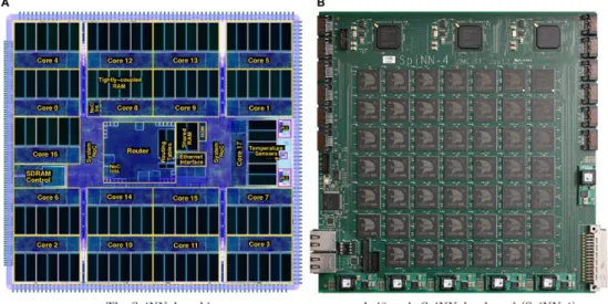
thread, block and grid) with their respective memory caches. ((Image fromhttp://www.training.prace-ri.eu/uploads/tx_ pracetmo/introGPUProg.pdfunder the Creative Commons 3 li-cense) . . . 15 1.6 On the left, the architecture inside a single SpiNNaker core. On

the right, the mesh organization of several SpiNNaker on board ((Image fromLagorce et al.(2015) under the Creative Commons 4 license). . . 25

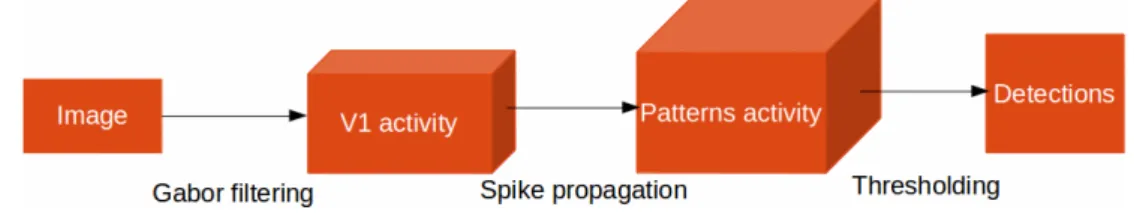
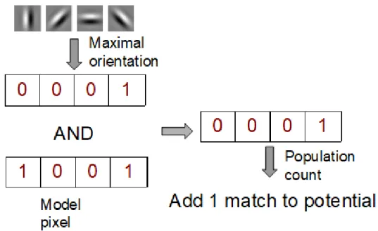
2.1 Principle of BCVision use cases . . . 32 2.2 Architecture of BCVision kernel process for a single image scale. 33 2.3 Binary propagation optimization in BCVision . . . 36 2.4 Example of images in the detection performance dataset. Left :

control image without transformations. Center : rotated image. Right : image with white noise. . . 38

(18)

2.5 Detection performances of the CPU and GPU versions of BCVi-sion on the Caltech-101 pasted images dataset. In red : the original CPU version. In blue : the GPU version without max-pooling. In green : the GPU version equipped with complex cells with stride s=2. In purple : the GPU version with max-pooling with stride s =4 . . . 41 2.6 Acceleration factor in seconds given the number of models on

a single scale 1080p image. The linear regression of processing times shows as the number of models grows the acceleration fac-tor converges toward 6.39. When the number of models is low, this acceleration is . . . 42 2.7 Max-pooling operation example. . . 44 2.8 The proposed BCVision architecture equipped with complex cells 47 2.9 The proposed coarse-to-fine detection architecture . . . 48 2.10 Detection performances of a coarse subsampled architectures given

two subsampling methods, model image rescaling prior to spikes generation versus spike-maps pooling . . . 49 2.11 Detection performances of the base GPU implementation of

BCVi-sion, the fully pooled models version and the coarse to fine ver-sion. The higher the score in each category, the most robust to the transformation the model. . . 51 2.12 Acceleration factor in millisecond given the number of models

on a single scale 1080p image with a fully pooled architecture version and the coarse-to-fine version of BCVision . . . 52

3.1 Binary dense propagation algorithm illustration . . . 61 3.2 Probability for a subpacket of size Sp = 32 to contain at least

one spike, as a function of M and N . . . . 64 3.3 Binary sparse propagation algorithm illustration . . . 66 3.4 Binary histogram propagation algorithm illustration . . . 71 3.5 Processing times of the binary dense algorithm in function of

M and N . In blue, real data point, in green the computational model estimation . . . 74 3.6 Processing times of the binary dense algorithm in function of M .

In red, real data point, in blue the computational model estimation 75 3.7 Processing times of the binary sparse algorithm as a function of

M and N . In blue, real data point, in green the computational model estimation . . . 76

(19)

3.8 Processing times of the binary sparse algorithm as a function of N . The different sets of points represent real data points, while the curves represent the computational model estimation. The colorbar maps the colors of the different curves to the correspond-ing value of M . . . . 76 3.9 Processing times of the binary sparse algorithm as a function of

M . The different sets of points represent real data point, while the curves represent the computational model estimation. The colorbar maps the colors of the different curves to the correspond-ing value of N . . . . 77 3.10 Processing times of the output indexes histogram algorithm as a

function of W . The different sets of points represent real data point, while the curves represent the computational model esti-mation. The colorbar maps the colors of the different curves to the corresponding value of N . . . . 77 3.11 Processing times of the output indexes histogram algorithm as

a function of N . The different sets of points represent real data point, while the curves represent the computational model esti-mation. The colorbar maps the colors of the different curves to the corresponding value of W . . . . 78 3.12 Processing times of the output indexes histogram algorithm as

a function of W and N . In blue, real data point, in green the computational model estimation . . . 78 3.13 Spike throughput comparisons between the three proposed

meth-ods. In red, the binary dense method, in blue the binary sparse method and in green the output indexes histogram method are shown. Each graph in a row corresponds to a single value of M , while each graph in a column corresponds to a single value of N . For each graph, the parameter W is represented on the x-axis, the spike throughput is represented on the y-axis. Note the spike throughput is represented using a log 10 scale. . . . 80 3.14 Probability that a subpacket of varying size Sp contains at least

(20)

(21)

(22)

Chapter 1 Context and state-of-the-art

Deep learning methods have recently shown ground-breaking performance levels on many tasks in machine learning. However, these methods have intrinsic con-straints which limits their industrialization. Such drawbacks are a direct conse-quence of the deep nature of the neural network used, which requires enormous amount of computations, memory resources and energy consumption. Several research projects attempt to solve this issue by finding ways to accelerate learn-ing and inference at software and hardware levels. One of the main advances that allowed allowed Deep Learning to become efficient and popular was the development of Graphical Processing units (GPU).

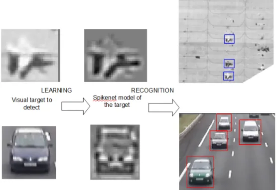
On the other hand, Brainchip Inc has used spiking neural network (SNN) based technology in order to perform fast visual pattern detection. Such networks, whose first purpose is the development of more realistic biological simulations, show interesting features for energy consumption reduction. As a matter of fact, BCVision, a software library for visual pattern detection developed in 2004 (under the name SNVision back then), is able to perform one-shot learning of novel patterns and detect objects by propagating information in the form of spikes. While BCVision is not as ubiquitous as Deep Learning methods, its principles are all biologically plausible, requires a low amount of data and require fewer resources.

This thesis proposes to explore the adequation of spiking neural networks and biological priors to parallel computing devices such as GPU. In this section we present the context of our research. We first show that the success of Deep Learning methods relies on processes similar to those seen in biological brains. We present next computational neuroscience models that are relevant for ex-plaining the energy-efficiency of the brain, and are marginally considered in the machine learning community. We also present research on GPU optimizations of both deep neural networks and spiking neural networks, as well as the GPU

(23)

programming model which will be of primary importance for the content of this thesis. We finally explore the current research trends in Deep Learning, in neural network hardware optimization and the relationship between machine learning and neuroscience.

1.1 Deep Learning methods and their links to

Biology

The fundamentals of Deep Learning

In the last decade, the machine learning community adopted massively Deep Learning methods, a set of algorithms based on neural networks architectures that can involve hundreds of layers. These methods have shown outstanding performances on many tasks in computer vision (Krizhevsky et al., 2012; He et al., 2016), speech recognition (Hannun et al., 2014; Amodei et al., 2016;

Zhang et al., 2017), natural language processing (Mikolov et al., 2013b,a) and reinforcement learning (Mnih et al., 2013; Gu et al., 2016; Mnih et al., 2016). Deep learning architectures use as a basis formal neurons (McCulloch and Pitts,

1943), derived from the perceptron model (Rosenblatt, 1958), a simple unit which performs a linear combination of inputs and their synaptic weights, fol-lowed by a non-linear function in order to compute its activation. Perceptron units are organized in layers, each layer receiving as inputs the activation from its previous layer(s). A network with multiple layers of perceptrons in called a Multi-Layer Perceptron (MLP). The Universal Approximator Theorem Cy-benko(1989) states that a two-layer MLP (with one hidden layer and an output layer) with a large enough number of neurons with sigmoid activation function can approximate any continuous function. It was also shown that only the non-linear behaviour of the activation function matters in order for an MLP to approximate any continuous function (Hornik, 1991).

Learning with a MLP is performed with the backpropagation algorithm in a supervised manner. The original article on perceptrons (Rosenblatt,1958) pro-posed a first learning algorithm which allowed the last layer of an MLP to learn a mapping between its inputs and a reference output (called labels or targets in the literature). However, this method did not provide a way to perform learning in multi-layer architectures. The backpropagation algorithm ( Linnain-maa, 1970; Werbos, 1982; Rumelhart et al., 1986; LeCun et al., 1988) allows a

(24)

multi-layer neural network to learn its internal representations from the error of prediction. Backpropagation is a gradient descent method, where for each input a feedforward pass through the neural network is performed in order to obtain a prediction. As each input is associated to a label (or target), the error of prediction is computed between the neural network prediction and the target. This error is then backpropagated through the network by the computation of each layer’s gradients from top to bottom, respectively to its inputs. Gradi-ent computations are based on the chain-rule (Dreyfus,1962), which allows the computation of the partial derivative of composition function. In other words, for a given parameter in the network (an activation or a synaptic weight), the chain-rule can approximate the error induced by this specific parameter given its inputs values and its output gradients. The main requirements for using backpropagation are the labelling of every input in the training dataset and the differentiability of every operation in the neural network. Note that this the last condition is violated with formal neurons (Rosenblatt, 1958), where activation function is a threshold (or Heavyside) function, which is non-derivable.

The development of such neural networks methods faced several obstacles be-fore. First, MLPs suffers a lot from the curse of dimensionality (Bellman,1961), meaning that with more input dimensions more neurons and samples are needed in order to avoid overfitting. Also before the extensive use of GPUs (Graphi-cal Processing Units) for Deep Learning, computation times were a significant issue, since a single training of a single feedforward neural network could take several days to weeks. As of today, such obstacles have been largely overcome as we shall see in the next section.

From MLPs to Deep Learning: biologically plausible priors

Multi-Layer Perceptrons suffer from operational drawbacks which hinder its ability to effectively approximate universally any continuous function as theo-rized by Cybenko (1989). We will see in this section how regularization tech-niques allowed artificial neural networks to overcome those drawbacks and to become the main method in machine learning. We show that many of these regularizations take inspiration from biological models of the brain, or at least have similarities to what can be found in biological neural networks.

(25)

Data availability It has been a common philosophy concern that the avail-ability of diverse observations helps humans to gain accuracy in their percep-tion of reality. Plato’s Allegory of the Cave states the impossibility for people with constrained observation scope to perceive correctly reality. Saint Thomas d’Aquin also proposed the concept of passive intelligence, the idea that human intelligence builds itself through experience of their environment. The more observation, the more a human or an animal is able to approximate reality, then take good decisions for its survival. This idea is supported by experi-ments in kittens showing that directional sensitivity (Daw and Wyatt, 1976) and orientation sensitivity (Tieman and Hirsch, 1982) can be modified during critical phases of their brain development by changing the environment. The fundamental laws of statistics and the curse of dimensionality both draw to the conclusion that an insufficient amount of data leads to variance problems, hence increasing the amount of data allows theoretically better generalization.

With the presence of huge amounts of data available via the Web, it has been possible to gather and annotate large datasets. For instance the ImageNet dataset (Deng et al., 2009), a famous dataset in computer vision, contains mil-lions of labelled images available for training. With the addition of random transformations and Drop Out (Srivastava et al., 2014) in order to artificially increase the number of samples, models are now able to generalize better. We should notice that even millions of samples are not sufficient in order to avoid the Curse of Dimensionality. Deep Learning systems may simply overfit the training dataset, but since they contain a huge number of configurations for each label, then it is able to generalize.

Convolutions Hubel and Wiesel (Hubel and Wiesel,1962) proposed a model

of hierarchical visual processing based on simple and complex cells. Simple cells are neurons with a restricted receptive field corresponding to a subregion of the field of view. Complex cells pool together visual information relative to an orientation over a patch, allowing robustness to translations, scaling and rotations of visual patterns. The HMAX model (Riesenhuber and Poggio,1999) implements a model on these principles that attempts to simulate processing in the ventral and dorsal visual streams. In the HMAX model, V1 simple cells are sensitive to oriented bars (Poggio and Bizzi,2004), while subsequent simple layers encodes all combination of inputs (for V2 all the possible orientation combination). Complex cells in HMAX apply a softmax operation in order to perform their pooling operation. However, this model has no ability to

(26)

learn novel visual representations in its intermediate layers, relying instead on a SVM classifier (Vapnik, 1999). The HMAX model is also slow in terms of processing times due to the number of potential combinations in all the simple layers from V2. Nevertheless, Serre et al. (2007) proposed a comparison of the HMAX model with a simple unsupervised learning scheme (synaptic weights of a randomly chosen unit are mapped to a random afferent vector) and human during an animal/non-animal classification task, and showed that such model behaviour is very closed to human’s one. It has also been shown that complex cells may not perform softmax operation for pooling, but rather a simple max operation (Rousselet et al., 2003; Finn and Ferster, 2007).

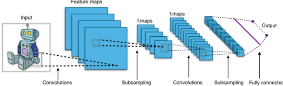
Artificial neural networks using simple cells with restricted receptive fields in-clude LeNet (LeCun et al., 1998), which performs handwritten digit classifica-tion on the MNIST dataset with high accuracy. LeNet relies on the convoluclassifica-tion operator in order to compute neural activations of simple cells, with one neu-ron’s receptive field being applied across all the spatial dimensions of the image. Convolutional Neural Networks (CNN) then uses weight sharing, the assump-tion that for a given output activity map, all the neurons associated to this activity map have the same synaptic weights over their receptive field. This as-sumption is wrong with respect to biology, but this approximation leads to two advantageous features for machine learning. Such constrained receptive fields allow the model to be more compact in memory, and also reduce the degree of freedom during learning since only a few synapses can be altered contrary to the fully-connected scheme typically used in MLPs. CNNs also have complex cells after each simple cell layer that performs max-pooling and subsampling neural activity over the spatial dimension further reducing both the computations and memory requirements for subsequent layers. Finally, in order to avoid runaway dynamics of the synaptic weights during learning, a weight decay (Krogh and Hertz, 1992) term is usually added to the update equation. The weight decay is a constraint on the norm of the synaptic weights. The most popular weight decay term is the L2-norm, and is also named Lasso in the statistics literature (Tibshirani,1996).

Activations Non-spiking neural models (McCulloch and Pitts, 1943;

Rosen-blatt,1958) have been equipped with diverse non-linearity functions like thresh-old, sigmoid and hyperbolic tangent (tanh) in order to approximate the rate of spiking in a non-linear regime. However, such non-linear functions, when dif-ferentiable, suffer a lot from the vanishing gradients problem when applying

(27)

Figure 1.1: Standard architecture of a convolutional neural network. (Image from https://commons.wikimedia.org/

un-der the Creative Commons 4 license)

backpropagation rule (Hochreiter et al.,2001), resulting in infinitesimal ampli-tudes of weight updates for the bottom layers in a hierarchy.

A biologically plausible non-linear behaviour relying on a simple piecewise-defined linear function was proposed by Hahnloser et al. (2000). This func-tion has been shown to correlate with physiological activity in MT cells (Rust et al., 2006) along with divisive normalization. The function assumes that if the activity of a neuron before the non-linearity is lower than zero, then the non-linear function outputs zero, else it outputs the given activity. Such acti-vation function have been later named Rectified Linear Unit (ReLU) (Nair and Hinton, 2010) and was successfully applied in Restricted Boltzmann Machines and Convolutional Neural Networks (Krizhevsky et al., 2012). The ReLU acti-vation function bypasses the vanishing gradient problem since its derivative for input values greater than zero is one, hence preserving the gradients amplitude.

Normalization Neural feedback inhibitions seem to play a role in contrast

invariance in many sensory circuits. Carandini and Heeger (1994) showed that excitatory-inhibitory circuits may implement a divisive normalization scheme (also known as shunting inhibition) in order to limit the effect of input variation in amplitude. The presence of such context-dependent normalization have been shown to occur in V1 cortcical circuits (Reynaud et al., 2012). As we have seen in the previous paragraph, shunting inhibition with a rectifier function correlates with biological recording of MT cells (Rust et al., 2006).

In the machine learning domain, special cases of normalizations are known as whitening processes. Whitening prior to propagation has been shown to help convergence during learning with back-propagation (Wiesler et al., 2011). In order to facilitate convergence in deep CNNs, the Batch Normalization method (Ioffe and Szegedy, 2015) mean-centers and scales by the inverse variance to

(28)

apply such whitening process. In Batch Normalization, the mean and variance statistics of each neuron is learnt over all the dataset and fixed for inference phase. Hence, statistics learnt with a given dataset may not be generalizable to another dataset. This issue was addressed by the proposal of Layer Normaliza-tion (Li et al., 2016) and Instance Normalization (Huang and Belongie, 2017) where the mean and the variance are computed online (thus not learnt) over the current batch or the current sample respectively. These different normal-ization schemes, while coarsely approximating biological neural normalnormal-ization, effectively reduce the number of iteration required for convergence.

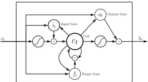
Recurrent neural networks The Long-Short-Term-Memory (LSTM) unit

(Hochreiter and Schmidhuber,1997) is a recurrent neural model equipped with gates, inspired from the ion channels in biological networks, which is able to learn long-term dependencies in temporal data. It is often used for natural language and audio processing. The Gated Recurrent Unit (GRU) (Cho et al.,

2014) is a simpler model of recurrent neuron which has been shown to perform equivalently to an LSTM unit.

Figure 1.2: Architecture of an LSTM neuron (Image from

https://commons.wikimedia.org/ under the Creative Com-mons 4 license)

(29)

1.2 Toward further biological priors for neural

network acceleration

In this section we consider several biological neural mechanisms which have emerged from neuroscience research and are rarely considered in the deep learn-ing literature.

A first mechanism is the spiking behavior of neural networks used in compu-tational neuroscience. The complete behaviour of spiking neurons have been described by Hodgkin and Huxley (1952) using electrical stimulation of squid nerves. Spiking neurons shows temporal dynamics according to their dendritic inputs. Input spikes are modulated by synapses’ conductance, and potentiation occurs at the soma. When the potential reaches a certain threshold, the neuron is depolarized and emits a spike along its axon, which is connected to other neu-rons dendrites. The Hodgkin-Huxley model of the neuron, while complete, is based on differential equations which computes the internal state of the neuron, thus resulting in a complex model. Simpler models are often used for simula-tion purposes, such as the Lapicque model (Abbott, 1999), also known as the leaky-integrate and fire (LIF) neuron. The LIF model captures the dot product behaviour between inputs and synapses, the thresold function and incorporate a leakage parameter. Izhikevich neurons (Izhikevich, 2003) also incorporate such behaviour in a very parametrizable manner and have been shown to reproduce many of the biological neural dynamics observed experimentally. The inter-esting factor of such neural models from a computational point of view is the nature of spikes, mathematically expressed as a Dirac distribution, or in the discrete case as a Kronecker of unit amplitude. We can assume that biological neurons output a binary information at each timestep, whether the threshold has been reached or not. This shows a fundamental difference between spik-ing neurons and LSTMs that encode information after the non-linearity as a floating-point real number. Spiking neurons also reset their potential right af-ter firing, where LSTMs only reset their activity given their inaf-ternal states and learnt gates weights. We can reasonably assume that spiking neurons may help in simplification of existing recurrent neural models.

Another interesting function of the brain is its ability to perform ultra-rapid visual categorization (Thorpe et al., 1996). Humans and primates are able to detect visual patterns in under 100 ms, leading to information being propagated during at most 10 ms in a single visual layer. The first wave of spikes is then probably sufficient for rapid visual categorization (Thorpe et al.,2001), since at

(30)

most one spike per neuron can occur in this 10ms frame. Rate coding is not able to explain such processing, since it cannot be measured with only one spike per neuron, thus spikes-timing coding is privileged for such task. As absolute timing differences are small, it was hypothesized through the rank order coding theory (Van Rullen et al., 1998; Thorpe et al., 2004) that a single spike per neuron is enough to perform rapid categorization of visual stimuli. In such framework, the absolute timing of spikes may be ignored, the relative order of the spikes being able to help discriminate different visual patterns. The adequacy of fully feedforward neural processing is also supported by the architectures of CNNs for computer vision tasks, where information in only propagated in a feedforward manner during inference. While CNNs typically compute neural activity as floating-points rates instead of binary spikes, we argue that rank order coding may provide useful constraints for accelerating deep learning methods applied to vision.

Figure 1.3: Latencies observed in each layer during a rapid visual categorisation task. (Image reproduced with permission

from Thorpe et al. (2001))

For spiking neural networks to learn representations, the backpropagation al-gorithm may not be applied since spiking behaviour are the result of a non-derivable threshold based non-linearity. Further more, it is biologically implau-sible that supervised learning schemes such as backpropagation could be the main learning mechanisms. Many representation appear to be learned in a un-supervised way, either by determined developmental functions (Ullman et al.,

2012; Gao et al., 2014), innate social learning behaviours (Skerry and Spelke,

(31)

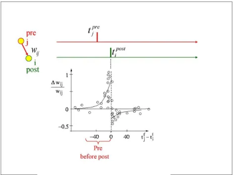
1997; Bi and Poo, 1998). One of the main unsupervised learning mechanisms occurring in the brain is called Spike-Timing-Dependent-Plasticity (STDP). STDP is a Hebbian learning rule based on the timing differences between pre and post-synaptic spikes. In machine learning terms, STDP acts as a spike-based coincidence detector and has been shown to allow neurons to rapidly learn novel representations and capture input statistics (Delorme et al.,2001;Perrinet and Samuelides, 2002; Guyonneau et al., 2005; Masquelier and Thorpe, 2007;

Masquelier, 2017). The adaptation of STDP to machine learning paradigm may serve the purposes of learning phase acceleration and bringing biological plausibility to deep networks.

Figure 1.4: Synaptic changes as a function of the spike timing difference of a pre and a post-synaptic neurone ((Image from

http://www.scholarpedia.org/under the Creative Commons 3 license)

1.3 Hardware dedicated to parallel computing

are suitable for neural networks

accelera-tion

We have seen in the previous section that regularization techniques allow arti-ficial neural network models to overcome their intrinsic issues. Regularization is generally implemented as model-based (or software-based) enhancement. In

(32)

this section we describe hardware-based enhancement brought by the algorithm-architecture adequacy of neural networks models on diverse devices, in partic-ular on Graphical Processing Units (GPU).

GPU acceleration of deep learning methods From the machine learning

perspective, the major breakthrough was the publication by Krizhevsky et al.

(2012), showing that is was possible to implement a deep convolutional neural network on a GPU: the famous AlexNet. The AlexNet architectures contains seven convolutional layers for a total number of 650 thousand neurons and 630 millions synapses. Such network on CPU would take far too long to train. The shift to GPU hardware allowed a drastic acceleration of processing times, and allowed the authors to train this network on two consumer-grade NVidia GTX 580 in less than a week for a hundred epoch on the whole ImageNet dataset. This represents an acceleration of an order of magnitude of ten. Since then, GPU have been massively adopted for deep learning. The different enhancement brought by NVidia to their GPU hardware and software library CUDA as well as the massive share of open-source code between academic and industrial actors in the field led to the rapid development and improvements of many Deep Learning framework like Caffe (Jia et al., 2014), Theano (Theano Development Team, 2016), Tensorflow (Abadi et al., 2015), MXNet (Chen et al., 2015) and many others as well as convenience wrappers.

GPU acceleration of biological neural networks On the computational

neuroscience side, different tools have been proposed in order to accelerate sim-ulations of biological neural networks. Frameworks like Brian (Goodman and Brette, 2009) and CarlSim (Beyeler et al., 2015) propose a unified design ar-chitecture of neural networks which can then be run on several devices such as CPU, GPU and dedicated hardware like IBM’s TrueNorth (Merolla et al.,

2014) and recently Intel’s LoiHi chip (Davies et al., 2018). The latter dedi-cated hardware pieces, while very energy-efficient, are research oriented, with a focus on biologically accurate simulations. Such simulations rely on very com-plex models, hence the possibility of deploying deep architectures on dedicated hardware and GPUs remain limited and does not fit operational requirements for applications. Finally, GPUs are far more accessible than dedicated hard-ware for both purposes, since they are basic components of computers and serve other purposes like other scientific and graphical computations for a lower price (considering consumer-grade GPUs).

(33)

CUDA programming model GPU technology has drastically improved over the last years, in terms of both computational efficiency and ease of de-velopment of such platforms. NVidia Corporation made several improvements in order to shift from their initial specialization on graphical processing toward scientific computations, and more particularly on neural network acceleration. With the addition of tensor cores (dedicated matricial computation units) on GPUs and convenient programming tools such as the CuDNN library for deep learning, Nvidia has taken the lead on the neural network accelerator market. AMD on the other hand was not as successful in this initiative, but strategi-cal shifts in their programming language from OpenCL to HIPs, which takes inspiration from the NVidia CUDA programming language and tries to unify programming on both platforms, make it possible for previously NVidia-only projects to be run on AMD platforms. Thanks to HIPs implementation of deep learning framework, recent benchmarks have shown that the recent AMD Vega architecture may perform better than NVidia GTX Titan X GPU in deep neural networks training (GPUEater, 2018). In this part we will describe the CUDA programming model in order to highlight the constraints inherent to parallel computing, since the new HIPs framework follows the same model.

NVidia GPUs require computations to be split between several parallel com-putation units called Streaming-Multiprocessors (SM). Each SM contains thou-sands of registers partitioned dynamically across threads, several memory caches to reduce memory access latencies (which will be detailed later in this section), a warp scheduler which quickly switches context between threads and issues instructions and many dedicated execution cores for different operations at var-ious resolutions (mainly using 32-bits integers and floating -points numbers).

SMs are designed to perform computations in a Single-Process-Multiple-Data (SPMD) manner, i.e. a single instruction is performed by the SM on each clock cycle on multiple different data points at the same time. In hardware, threads are organized in warps, a warp being a set of 32 threads performing the same computation. Instructions are issued to dedicated units, which can vary in terms of performances depending on the bit resolution and the nature of the operation. For instance, 32-bits integer additions can be performed on a single SM in four clock cycles, but the compute-units can pipeline processing and process four warps at the same time. The efficiency of an operation is given by its throughput, which is roughly the amount of data on which the operation can be performed on one clock cycle. In our example, the throughput of the integer addition is 128, since four warps can be pipelined at the same time on

(34)

the dedicated compute unit.

Data transfer between the host memory (the RAM module) and the SM is divided between several memory-cache layers.

• The global device memory is the largest but slowest memory space em-bedded on the GPU. As of today its capacity can reach dozens of gigabits of data. Data transfers are done through PCI-Express port (where PCI stands for Peripheral Component Interconnect), hence the data rate trans-fer between the host and the global memory is limited to 20 Gbits/s. Also, this memory currently relies on GDDR5 (Graphical Double Data Rate) or HBM2 (High Bandwidth Memory) technologies, on which read and write instructions from SM have longer latencies than on classical CPU architectures. From the GPU perspective, data are accessed through large memory buses (256 to 384 bits for GDDR5, 2048 to 4096 bits for HBM2) by loading large chunks of aligned and coalesced memory spaces. This is a major constraint of the parallel programming model as the violation of memory access patterns induces long latencies. Much care should also be taken regarding concurrent writes in global memory, which can result in data inconsistency. Atomic operations, i.e. writing in a memory location in a thread-safe manner, are supported but also increase latency. Such operations should not be used extensively in order to keep the advantage of parallel processing on computation times.

• When data chunks have to be accessed in a read-only fashion, the texture cache memory allows those chunks to be accessed more rapidly and reduces the latencies induced by uncoalesced accesses. Such texture cache is highly optimized for 2D and 3D memory reading and can be very useful for algorithms where data is read from neighbouring spatial locations.

• The constant memory is able to store a few dozen Kilobytes of data and is able to rapidly transfer its content to SM. Transferring data to constant memory is however slow. This memory is then useful for global parameters shared between threads.

• The shared memory is a block of dozens of kilobytes (typically 64kB) em-bedded in each SM. This memory is accessible by all the threads running on a given SM. As shared memory is highly optimized for low latency data transfer between threads, this memory is practical for reduction al-gorithms (summing, max, sorting) and local atomic operations. Data in shared memory is organized in 32-bit memory banks. There are 32 banks

(35)

per SM, allowing each bank to store multiple 32-bits values. Accessing different values in the same bank is inefficient since it leads to bank con-flicts. Shared memory is nevertheless efficient for coalesced accesses or for broadcasting values over multiple threads.

• There are also thousands of registers per SM on which computations are directly applied. For recent architectures the number of registers can reach 65536 per SM, and 255 registers can be assigned to each thread. Registers are 32-bits in size.

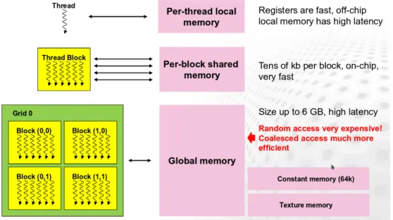
On the software side, functions are implemented from a thread perspective and are named kernels. A kernel describes all the computations done by a single thread. Kernels are launched on the GPU following a launch-configuration given by the developer. The launch-configuration informs the GPU on how the computations are organized across threads, blocks and grid. Blocks are a group of at most 1024 threads which are run on a SM and can hence access the same shared memory chunk. Threads can be organized over three dimensions x, y, and z, with the product of the three dimensions being the total number of threads in that block. The grid informs the GPU on the number of blocks that must be launched, and is also organized in three dimension. The division into three dimensions is useful for multi-dimensional algorithms. This organization is important since data transfers between threads and synchronizations can only occur within the same block. Indeed, it is impossible to have a global synchronization barrier between blocks., i.e. for a single kernel launch, threads belonging to one block are unable to communicate any data with the threads from other blocks. If such global synchronization is required, the kernel have to be launched multiple times, inducing launch overheads.

From these considerations, a few golden rules can be raised. First, data transfers between the different GPU memory layers have to be limited. Access patterns should be performed in an aligned and coalesced fashion. Also, high throughput computations must be privileged. This is often reduced in a single rule of parallel computing: hide the latencies.

(36)

Figure 1.5: The CUDA threads organization across the three levels (single thread, block and grid) with their respective mem-ory caches. ((Image from http://www.training.prace-ri. eu/uploads/tx_pracetmo/introGPUProg.pdf under the

Cre-ative Commons 3 license)

1.4 State-Of-The-Art

Recent advances in Deep Learning

Generative adversarial networks Generative Adversarial Networks (GANs)

(Goodfellow et al., 2014) have been said the most interesting idea in machine learning in the last decade according to Yann LeCun. GANs are a method for learning a generative model with an adversarial process, a mini-max game between two networks: a generator and a discriminator. The discriminator is trained for a classification task between real and fake data distribution. The generator’s purpose is to generate samples which belong to the real data distri-bution by using the discriminator gradients. The metaphor of two networks try-ing to fool (or beat) each other illustrate the adversarial nature of such method. This method has become popular for its ability to produce very realistic samples from different image datasets.

Since GANs were first proposed in 2014, research on GANs have become nu-merous (hindupuravinash, 2018). Many researchers focus on stability problems of GAN. In original research, the generator or the discriminator can become better at its specific task than the other, leading to a point where the whole network does not learn anything else. Also, GANs suffer from the mode-collapse issue, where generated images can lack in variation or worse, the generator may

(37)

learn some specific samples from the training dataset. This was adressed first with DC-GAN (Radford et al., 2015), which proposed a very stable architec-ture for image generation, as well as showing that feaarchitec-tures learnt by GANs are relevant for unsupervised pre-training. It was able to generate faces and house interiors realistically. Improvements in GAN training (Salimans et al.,

2016) have leveraged stability and generated image sizes from 64 pixels to 256 by proposing feature matching, minibatch normalization and avoiding sparse gradients in their models. WGAN (Arjovsky et al., 2017), Improved-WGAN (Gulrajani et al.,2017) and DRAGAN (Kodali et al.,2018) propose other vari-ation of the loss function based on the Wasserstein Distance (Vaserstein, 1969). Experimental results have shown improved stability and reduced mode-collapse.

By mixing GANs and auto-encoders architectures, applications involving arti-ficial data generation have been widely explored. For instance:

• Faces generation (VAE-GAN (Larsen et al., 2015), DC-GAN (Radford et al., 2015))

• Super Resolution (SR-GAN (Ledig et al.,2016), 512 pixels faces (Karras et al., 2017))

• Image to Image translation (CycleGan (Zhu et al.,2017), StarGan (Choi et al., 2017))

• Realistic drawing from pixels(Pix2pix (Isola et al.,2017)) • Text to image (Reed et al.,2016)

• Music and voice generation (WaveNet (Van Den Oord et al., 2016))

Deep reinforcement learning Training AI as an agent in a complex

en-vironment is one of the most difficult tasks. Indeed, the greedy state-space exploration (with backtrack algorithm for instance) is out of question in such environments since the number of possible states needed to achieve human-like performances can rapidly explode. While greedy exploration has been shown to be efficient for some games, for instance with IBM DeeperBlue beating Garry Kasparov at chess, games like Go or current video-games face an explosion in the number of configurations and thus backtrack algorithm would take far too much time to take any decision. Instead, methods trying to approximate good solutions by learning over many iterations can overcome this issue. Such methods try to infer an action using the environment state as the input.

(38)

Evolutionary algorithms are methods based on parameters combining between the most successful agents in a population tested with a given environment. These methods are designed to mimic hereditary transmission of successful behaviours through generations. Sub-classes of evolutionary algorithms in-clude evolution strategies (Rechenberg,1965), evolutionary programming (Fogel et al.,1966), genetic algorithms (Fogel,1998) and memetic algorithms (Moscato et al., 1989). Such approaches have been shown to be fairly efficient for many tasks, including autonomous car driving (Togelius et al., 2007), mobile robots (Valsalam et al., 2012) and gaming (Togelius et al., 2011). However until re-cently, the performance of such methods was not high enough for operational deployment.

On the other hand, back-propagation methods allow training of a single model agent through Reinforcement Learning (RL). RL is designed to mimic Pavlovian-like training. Such training uses reward and punishment signals in order to learn through experience. With the breakthrough of deep learning, Deep Re-inforcement Learning (Mnih et al., 2015) (DRL) have been able to leverage current AI research in a range of tasks. Deep Q-Learning research (Mnih et al.,

2013) showed near human performances on several Atari games with a single AI architecture. Deep reinforcement learning techniques also allowed the AI AlphaGo to beat the world champion of Go, Lee Sedol (Silver et al., 2016). This achievement is remarkable since the game of Go is a board game with 250150possible combinations and so considered to be a very difficult game. Au-tonomous car-driving is also currently in the spotlight of applicative research in deep reinforcement learning (Kisačanin,2017). While deep Q-learning can only be trained on one environment at a time, the Asynchronous Advantage Actor Critic (A3C) method (Mnih et al., 2016) recently allowed a single agent to be trained with multiple agents asynchronously, allowing scaling of the training-phase for multiple devices.

While DRL techniques seem to outperform evolutionary algorithms, recent pub-lications show that efficient parallel implementations of evolutionary strategies can reach equivalent performance levels faster (Salimans et al., 2017). Even gradient-less approaches like genetic algorithms can be competitive with such parallelization (Such et al., 2017). We can see here that algorithm-architecture adequacy can be the main factor for optimizing performance.

One should note that autonomous agent research is currently easily accessi-ble. OpenAI, a non-profit AI research company, developed a publicly available toolkit for reinforcement algorithms called Gym (Brockman et al.,2016). Gym

(39)

can emulate environments for Atari games, autonomous driving cars and ad-vanced video games such as Doom and Grand Theft Auto 5. Such open-source initiatives mean that we can expect research in autonomous agents to progress rapidly.

Neural network quantization Inference with deep neural networks can be

energy-consuming as computations rely on 32-bit floating-points values. The consequences are high-memory usage for data and models. In order to reduce such storage problems, a lot of research on deep neural network has looked at the impact of quantization. For example, a 32-bit value may encode up to 32 binary values, thus potentially compressing models by a factor 32. Also, in a binary framework, the dot product operation is equivalent to a bitwise XNOR and a population count operation on 32 values at the same time, resulting theoretically in sixteen times fewer computations. Finally, as shown by Seide et al.(2014), gradients quantization down to 1-bits can also be advantageous for reducing network transfers between different devices during learning, allowing better scaling during this phase.

One way to perform parameter quantization is by reformulating deep learning in a probabilist framework. By doing so, Expectation backpropagation (Soudry et al., 2014; Cheng et al., 2015) can be applied instead of the usual gradient-descent error backpropagation, allowing the training of multi-layer perceptron networks with binary weights. Networks trained with expectation backpropa-gation show performances equivalent to full-precision networks on the MNIST dataset. However, Expectation Backpropagation has not been applied on deep convolutional architectures. Whether it is possible or not is still an open ques-tion.

Many recent publications show that training quantized neural networks with backpropagation is possible. The BinaryConnect method (Courbariaux et al.,

2015) proposes to train neural networks with binary networks by using the binary projection of real-value weights during the feedforward and backward steps. The binary projection is performed by applying the hard-sigmoid func-tion, which is linear between -1 and 1, equal to 0 for input values lower than -1 and equal to 1 elsewhere. Once the gradients with respect to the binary weights have been computed, the real-value weights are updated with respect to the partial derivative of the hard-sigmoid function. With such methods, BinaryConnect networks show equivalent performance levels to networks with real-valued weights.

(40)

BinaryNet (Courbariaux et al.,2016) is an extension of BinaryConnect in which the same principle of binary projection is applied to activations. A neural net-work trained this way has all its activations and weights binarized. The ar-chitectures rely on successive layers of convolution, batch normalization and hard-sigmoid (or hard-tanh in some cases). However, quantization of both ac-tivations and weights induce a substantial performance loss on classification tasks such as MNIST, SVHN and CIFAR-10. For operational deployment, only the binary weights and batch normalization learnt mean and variance values need to be kept, hence resulting in effective compression of the model. Also, this article reported an acceleration factor of 7 with an unoptimized GPU ker-nel. Since batch normalization parameters are constant at inference, this step as well as binarization can be theoretically performed within the same kernel as the convolution, hence resulting in further acceleration factor due to the reduced memory overhead. Also, this architecture has been implented on dif-ferent architectures (CPU, GPU, FPGA and ASIC) in order to evaluate the potential acceleration factor on these different architectures (Nurvitadhi et al.,

2016). Not surprisingly, ASICs deliver four orders of magnitude acceleration factor, FPGAs three orders of magnitude and GPUs two orders of magnitude. The paper discusses whether better fabrication processes for FPGA as well as hardened parts and Digital Signal Processor (DSP) may close the gap with ASIC in terms of acceleration and energy-efficiency.

In order to extend quantization to different resolutions, the DoReFaNet frame-work (Zhou et al., 2016) proposed different projection functions for weights, activations and gradients which allows any resolution, which is defined prior to training as a hyper-parameter. The article shows that performance levels equivalent to full precision networks can be achieved with the AlexNet archi-tecture (Krizhevsky et al.,2012) using 1-bit weights, 2-bit activations and 6-bit gradients on the ImageNet classification taks. It also shows that different tasks require different resolutions, since further quantization was achieved on the SVHN dataset.

The XNOR-Net method (Rastegari et al., 2016) allows deep neural networks to be trained using binary activations, weights and gradients. It approximates float-based convolutions with a binary convolution and an element-wise product busing a scalar α (the average of absolute weight values) and a 2D matrix K (the spatial mean of the input over the kernel fan-in). Gradients are computed during the backward step with a hard-tanh projection. With an additional floating-point overhead compared to BinaryNet, performances are almost equivalent to

(41)

full-resolution networks. The authors also report an effective 32 fold memory saving and 58 times faster convolutional operations.

Ternary networks training (Zhu et al., 2016; Deng et al., 2017) has also been studied. Compared to binary networks, ternary networks reach the same level of performances as their floating-point equivalent networks. Ternary networks are less difficult to train and perform better than binary networks in general.

The state-of-the-art in neural networks quantization shows that binary networks can drastically accelerate processing times although this is at the expense of performance. Keeping some information as floating-point values or having a ternary quantization instead can reduce the performance loss. In any case, the quantization parameters have to be chosen considering a trade-off between ac-celeration and performance. One should note that in all the previous research, only classical feedforward architectures have been benchmarked. Advanced ar-chitectures such as Residual networks (He et al., 2016), Inception networks (Szegedy et al., 2017), recurrent architectures (GRU and LSTM) and GANs have not been trained with such quantization for now. Since these advanced architectures reach the state-of-the-art, current quantization-schemes also suffer from architectural limitations impeding the best models to be accelerated this way.

Advances on large-scale simulation technologies

Available software for Deep Learning The first efficient and modular

implementation of convolutional neural networks with GPU support, cuda-convnet, came from Alex Khrizhevsky prior to his victory in the ImageNet competition (Krizhevsky et al., 2012). The software architecture adopted re-lied on a list of layers defined in a configuration file, which processes batches of images and updates their parameters iteratively. This architectural design only allowed a single input and output per layer, but the development of the Caffe framework (Jia et al., 2014) allowed the definition of a global graph of layers. Caffe became very popular thanks to the abstract classes it proposed, allowing much more modularity and custom implementations. Caffe is writ-ten in C/C++ with CUDA support and different high-level wrappers (Python, MatLab), hence demanding advanced development skills if used in the context of research at the level of layers. Nevertheless, the attained trade-off between modularity and computational efficiency of Caffe made the framework popular in both academic and industrial communities.

(42)

Before this neural networks revival in 2012, libraries such as Theano1 (Bergstra et al.,2010) and Torch (Collobert et al.,2002) had been developed for machine learning purpose. Theano is presented as a mathematical expression compiler for Python language. It can perform efficient vector-based computations in the same way as the Numpy library and Matlab, and perform code compilation and optimization at run-time in order to maximize the speed of processing. Compilation is performed when creating functions, which take as parameters a set of input and output place-holders as well as an optional parameters update expression (typically used for updating weights in neural networks at each step). Development with Theano is oriented toward functional-programming, where a function is a graph of transformations given one or several input tensors. Theano targets researchers more than Caffe since the first one allows tensor programming while the second allows layers programming. One should note that the Torch library also allows such tensor-based programming but does not perform run-time compilation yet.

The functional design of Theano and Torch with convenient layer-based classes inspired the many industrially-developed frameworks for machine learning. Among these libraries we can mention TensorFlow (Abadi et al.,2016) , Pytorch (Ketkar,

2017), Nervana, MXNet (Chen et al., 2015), CNTK (Seide and Agarwal,2016) and Caffe2 (Goyal et al.,2017). As of today, Tensorflow is the framework with the most active community. Keras (Chollet et al.,2015) is also worth a mention since it provides a high-level abstraction for training deep neural networks us-ing Theano and Tensorflow back-ends, allowus-ing both code portability between the two frameworks and fast-development. We can also note that a major part of these frameworks are backed by industrial groups and released with a free and open-source license on Github, allowing for fast improvements with active participation from the community.

NVidia also provides active support for their GPU-devices. As AlexNet popular-ized NVidia GPUs with cuda-convnet (Krizhevsky et al., 2012), the company released in 2014 the cuDNN library, which provides optimized functions for standard deep learning. CuDNN is extensively integrated in almost every deep learning framework. NVidia also developed TensorRT, a C++ library which quantizes floating-point networks trained with Caffe to 8-bit integer versions that accelerate inference by a factor of up to 48.

Since deep learning literature has grown rapidly, proposing several methods,

(43)

software development for machine learning is essentially focused on the im-plementation of these novel methods, as well as convenient abstractions and distributed computing to facilitate learning and inference.

Dedicated hardware for Deep Learning As NVidia GPUs are the main

hardware for deep neural networks , the company proposed in the latest Volta architecture (Tesla V100) dedicated computation units for 4 × 4 × 4 matrix multiply-add operations using 16 to 32-bit floating-point values. This results in 64 floating-point multiply-add per clock cycle per core, with eight cores per SM. NVidia claims this dedicated units achieve an acceleration of 8 per SM compared to the earlier Pascal GP100 architecture. Considering V100 GPU has more SM and more cores per SM, the achieved increase in throughput is twelve times compared to the previous generation.

Google has also developed its Tensor Processing Unit (TPU) technology (Jouppi et al.,2017) to accelerate deep learning inference for its cloud offers. Like GPUs, TPUs are PCI-E boards with an ASIC specialized for TensorFlow routines, particularly for neural network processing. The board includes a DDR3 RAM memory for weight storages as well as local buffers for storing activations and accumulations. The dedicated units are specialized for matrix-multiplication, activation functions, normalizations and pooling. Google reports the device can perform 21.4 TFLOP/s (averaged over diverse neural architectures) for 40W power-consumption.

NVidia has also proposed solutions for embedded GPU architectures, the first generation being the Tegra K1 (TK1) with 256 CUDA cores connected to an ARMv15 processor. The second generation, the Tegra X1 (TX1), features 512 cores embedded on the device delivering up to 313 GFLOP/s for a maximum power consumption of 15W. It is possible to combine TensorRT models on TX1 to run computer vision applications in real-time in an embedded system. An alternative way to embed deep learning based applications are provided by In-tel (with its Movidius chips) and GyrFalcon Technology. The two companies propose specialized USB devices which contains dedicated compute units. For instance, the Intel Movidius (Myriad 2) device embed 2Gb of RAM memory with twelve vector-processors (sixteen for their latest product, the Myriad X), which are units specialized in 128-bit based computations (able to process four floats or integers, eight half-float or sixteen 8-bit words in parallel). USB de-vices consumes 1W of memory for 100 GFLOP/s and are fully compatible with nanocomputers like Raspberry Pi and Odroid. In terms of performance per

(44)

watt and prices, the USB-device solution for embedded deep learning applica-tions seems the best as of today.

Available solutions for SNN simulation Several frameworks are available

for simulating large-scale spiking neural networks. Software frameworks exam-ples: NEURON (Carnevale and Hines, 2006), GENESIS (Wilson et al., 1989), NEST (Hoang et al., 2013) and BRIAN (Goodman and Brette, 2009). These frameworks are designed and maintained with modularity and scalability pur-poses. They are able to handle simple neural models such as LIF and Izhikevich Neurons, complex ion-channels dynamics and synaptic plasticity. The database ModelDB (Hines et al., 2004) proposes a collection of models shared between researchers, using such frameworks.

Because spiking neural networks simulations are directed toward biological plau-sibility, models tend to be far more complex than those in Deep Learning. Hence processing times are critical for research efficiency, mainly because of the dif-ficulty to tune SNN dynamics parameters. For such work, methods based on genetic algorithm or Runge-Kutta optimizations are used, but require several simulation run before convergence.

Many efforts were deployed in order to accelerate processing for such simula-tions. NeMo (Fidjeland and Shanahan, 2010), BRIAN, Nengo (Bekolay et al.,

2014), GeNN (Yavuz et al.,2014) and CarlSim (Beyeler et al.,2015) have GPU-processing capabilities. Brian, Nengo and NEST also have distributed comput-ing options, allowcomput-ing large simulations to be run on clusters. Given the different features of the all these simulation frameworks, PyNN library (Davison et al.,

2009) allows a unified approach of SNN model definition and makes it possible to run models on different frameworks (currently wih Brian, Nengo and NEST), but also on neuromorphic devices and specialized clusters.

Neuromorphic hardware While the brain process information through

bil-lions of computation units in parallel, nowadays computers rely on the Von Neumann architectures, where computations are performed sequentially with an externalized memory accessed from a bus. The difficulty of running large-scale simulations of biological neural networks comes from this drastic difference between the brain and the Von Neumann architectures. In this sense, a lot of research is directed toward neuromorphic architectures in order to reach the speed and energy efficiency observed in the brain.