Dynamique spatio-temporelle des populations de
canards barboteurs et de leur habitat
Thèse
Christian Roy
Doctorat en sciences forestières
Philosophiæ doctor (Ph.D.)
Québec, Canada
iii
Résumé
Le principal objectif de ma thèse était de quantifier la variation spatiale des populations de canards barboteurs et de leur principal habitat de reproduction, et d'évaluer l'importance de cette variabilité. J’ai d’abord réalisé une étude de cas sur le Canard colvert (Anas platyrhynchos) qui visait à évaluer l’impact de l’utilisation de priors informatifs sur un modèle de population de Gompertz spatialement explicite. Pour ce faire j’ai comparé les résultats d'un modèle naïf et d'un modèle où j’ai restreint les taux de croissance intrinsèques (r) des populations à des valeurs biologiquement réalistes. Le modèle naïf présente des taux de croissances intrinsèques irréalistes et des temps de retour à équilibre beaucoup plus court que ceux présentés dans le modèle informé. Par la suite, j’ai évalué les variations spatiales des facteurs climatiques qui influencent l’abondance des fondrières dans les Prairies. Les précipitations à l’automne et au printemps sont les facteurs les plus importants dans l’ouest tandis que les précipitations durant l’hiver et l’été sont les facteurs les plus importants dans l’est. J’ai par la suite développé une extension multivariée du modèle de population pour évaluer la synchronie dans les populations de quatre espèces de canards barboteurs de l’ouest du continent: le Canard colvert; le Canard pilet (Anas acuta); le Canard d'Amérique (Anas americana); et la Sarcelle d'hiver (Anas crecca). Les populations de Canards pilets et de colverts dans les prairies sont négativement corrélées avec les populations dans le nord de la forêt boréale et de l'Alaska ce qui renforce la thèse selon laquelle une partie de ces populations « survolerait » les prairies pendant les années de sécheresse. Finalement, j’ai évalué la variabilité spatiale et temporelle du taux de récolte de Canard noir (Anas rubripes) sur leur habitat de reproduction canadien à l’aide de données de baguage. La probabilité de récupération des bagues est corrélée avec l’effort de chasse pour les juvéniles, mais je n’ai pas détecté d’impact de l’instauration de la réglementation de récolte plus stricte au début des années 1980. Les taux de récolte le long du fleuve Saint-Laurent et dans les provinces de l'Atlantique demeurent particulièrement élevés et devraient être étroitement surveillés pour éviter la surexploitation
v
Abstract
The main objective of my thesis was to quantify the spatial variation in duck populations in North America and their main breeding habitat and assess the importance of this variability. I first present a study case on the Mallard (Anas platyrhynchos) that aim at assessing at how using informative priors on population parameters effects the conclusions drawn from a spatially explicit Gompertz population model. I compared the results from a naïve model and from a model where I constrained the intrinsic growth rate (r) to biologically realistic values. The naïve model lead to the estimation of unrealistic growth rate and shorter return time to equlibirum than those estimated by the informed model. The effects of the extrinsic factors were however comparable across both model. I subsequently used a spatially-varying coefficients model to assess the spatial variation in the ecological drivers of wetlands abundance in the Prairies pothole region (PPR). Overall, fall and spring precipitation were the most important climatic drivers in ponds abundance in the west while winter and summer precipitation and the most important driver in the east. Based on my previous results, I developed a multivariate extension of the Gompertz population model to assess the synchrony and the spatial variation in populations dynamics of four species of dabbling duck: the Mallard; Northern Pintail (Anas acuta); American Wigeon (Anas americana); and Green-winged Teal (Anas crecca). Northern Pintails and to a lesser extent Mallards showed a pattern of negative correlations among populations in the PPR and populations in the Western boreal forest of northern Canada and Alaska supporting the contention that some individual will “overfly” the PPR during drought years. Finally, I assessed the spatial and temporal variability in harvest rate of American Black Duck (Anas rubripes) on their Canadian breeding ground with direct recoveries from banding data. Juveniles recovery probabilities were correlated with the hunter effort but did not decreased after the implementation of new, stricter, harvest regulations in the early 1980’s. Harvest rate along the Saint Lawrence River system and in the Atlantic Provinces remain particularly high and should be closely monitored to avoid overexploitation.
vii
Table of content
Résumé ... iii
Abstract ... v
Table of content ... vii
List of tables ... xi
List of figures ... xiii
List of appendices ... xvii
Remerciements ... xix
Avant-propos ... xxi
General Introduction ... 1
Dabbling duck ecology ... 1
Waterfowl management ... 2
Population dynamics ... 4
Spatial hierarchical models ... 5
Methodological approach ... 7
Chapter 1 Unbiasing estimates of density dependence in time series data: a case for the use of informative priors ... 11 Abstract ... 12 Résumé ... 13 Introduction ... 14 Methods ... 16 Population data... 16 Climatic data ... 17 Model ... 18 Process-model ... 18
Spatial Population Model ... 19
Informative priors ... 20 Model fitting ... 21 Results ... 21 Mean effects ... 21 Spatial process ... 23 Spatial coefficients ... 24 Discussion ... 28
viii
Naïve model vs Informative prior ... 28
Continental Mallard population dynamics ... 29
Implications for Managing Mallard Populations ... 30
Conclusion ... 31
Acknowledgements ... 31
Appendices ... 32
Chapter 2 Quantifying the geographic variation in the climatic drivers of midcontinent wetlands with a spatially varying coefficient model ... 37
Abstract ... 38
Résumé ... 39
Introduction ... 40
Material and methods ... 42
Pond data ... 42
Explanatory variables and Expectations ... 43
Climatic data ... 44 Model ... 44 Model estimation ... 46 Derived parameters ... 46 Results ... 47 Mean effects ... 47 Spatial parameters ... 49 Discussion ... 54
Temporal lag and precipitations ... 54
Temperature ... 55
Temporal trend in pond abundance ... 55
Implications for climate change... 56
Limitations of the dataset ... 57
Conclusion ... 57
Acknowledgement ... 58
Appendices ... 59
Chapter 3 Population synchrony of dabbling ducks in western North America ... 61
Abstract ... 62
ix Introduction ... 64 Predictions ... 66 Methods ... 67 Population data... 67 Habitat data ... 69 Population model ... 69 Results ... 73 Mean effects ... 73 Population parameters ... 73 Extrinsic factors ... 75 Population synchrony ... 79 Discussion ... 81 Population parameters ... 82 Extrinsic factors ... 82 Population synchrony ... 84 Conclusion ... 84 Acknowledgements ... 85 Appendices ... 86
Chapter 4 Spatial and temporal variation in harvest probabilities for American Black Duck ... 93
Abstract ... 94 Résumé ... 95 Introduction ... 96 Methods ... 98 Banding data ... 98 Recovery probability ... 99
Proportion of recoveries in Canada ... 100
Estimation ... 101
Derivation of harvest probabilities... 102
Results ... 103
Recovery probability ... 103
Proportion of recoveries in Canada ... 105
Harvest probabilities ... 107
x
Recovery probability ... 109
Proportion of recoveries in Canada ... 110
Spatial variation in harvest probabilities ... 110
Temporal variation in harvest probability ... 111
Conclusion ... 112
Acknowledgement ... 112
Appendices ... 114
General Conclusion ... 117
Synthesis of the main results ... 117
Application of the main results ... 119
Future perspective ... 120
xi
List of tables
Table 2.1 Summary for the mean effect (𝜇) of explanatory variables, the associated standard deviation (𝜎). ... 49
Table 3.1 Mean effect (𝜇) of the density dependent term, extrinsic factors regression terms, associated standard deviation (𝜎) parameters, and the spatial range (𝜙) and effective spatial range (√3𝜙) in each direction. ... 74
Table 3.2 Distribution of the pair-wise correlations among stratum-level populations that do not include zero in
their 95% Credible Intervals in function of distance class and the direction of the correlation (+/-) for each species. Distance class labels indicate the upper bound of the distance class ... 80
xiii
List of figures
Figure 1.1 Study area and strata (n=51) used for the analysis. Shading represents waterfowl sub-regions
adapted from Boyd (1991). Numbers indicate strata numbers. ... 17
Figure 1.2 a) Histogram of the empirical distribution of the intrinsic growth rate estimated by the demographic
invariant approach and probability density function of the approximate Normal prior used in the informative prior; b) Posterior distributions the mean intrinsic growth rate (𝜇𝑟) estimated by the naïve model c) standard deviation for the intrinsic growth rate (𝜎𝑟) estimated by the naïve model. The dotted grey line in b) and c) represent the value used in the informative model. ... 22
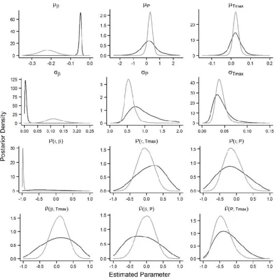
Figure 1.3 Posterior distributions of the mean (μ), standard deviation (σ) of and correlations among (ρ) model
parameters for the naïve model (grey line) and informative prior model (black line). The correlation among the model parameters is estimated via the variance-covariance matrix T (Eq. 1.8). ... 23
Figure 1.4 Scatterplots of stratum-level means for intrinsic growth rate (r) and the return times to equilibrium
(1/-β) within the naïve model (a) and the informative prior model (b). Scatterplots of the stratum-level
estimates of the variance of the stationary distribution of population fluctuation (𝜎𝑁2) and the carrying capacity (K) for the naïve model (c) and the informative prior model (d). Confidence intervals were omitted for clarity. Note the differing y-scales between the naïve and informative model plots. ... 25
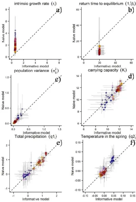
Figure 1.5 Relationships between the per-strata population parameters estimated by the naïve model and the
informative prior model (a-d). Relationships between the estimated parameters for the extrinsic factors in the naïve model and the informative prior model (e,f) Light grey lines represent the 95% credible intervals while the dashed line (all panels) represents a perfect correlation (intercept 0 and slope 1). ... 26
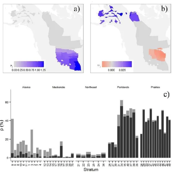
Figure 1.6 a) Mean regression coefficient for total precipitation in the informative prior model; b) mean
regression coefficient for spring maximum temperature in the informative model. For both variables the strata which include 0 in the 95% credible interval are presented as grey; c) proportion of the variance explained by environmental variables in each strata for the informative prior model. The dark grey bar represent the proportion of variance explained by the precipitation during the previous year while the light grey bar represent the proportion of variance explained by temperature in the spring ... 27
Figure 2.1 Map of the Waterfowl Breeding Population and Habitat Survey area with numbers indicating survey
strata used in the analyses (n=24); AB=Alberta, SK=Saskatchewan, MB=Manitoba, MT=Montana; ND=North Dakota; SD=South Dakota. ... 42
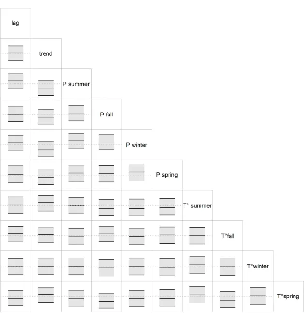
Figure 2.2 Each rectangle presents the posterior distribution of the correlation parameter between the
predictors. Plotting areas range between -1, and 1, the dashed grey lines indicates 0, and the black lines represent the median estimate and the upper and lower 95% Credible Intervals. None of the estimated correlations are significantly different from 0. ... 48
Figure 2.3 Geographical variation in the stratum level, mean pond density(𝑒𝛽0+𝜎22⁄km2), and the predicted coefficient of variation (√𝑒𝜎2
− 1) for pond abundance in the survey area. ... 50
Figure 2.4 Geographical variation in the estimated effects of pond abundance in the previous year (Lag) and
the linear effect of time (Trend). In strata where the 95% Credible Intervals for a coefficient included 0, the effect is considered insignificant; these strata are coloured grey. ... 50
xiv
Figure 2.5 Geographical variation in the predicted effect of seasonal precipitation during the previous year on
pond abundance. In strata where the 95% Credible Intervals for a coefficient included 0, the effect is
considered insignificant; these strata are coloured grey. ... 51
Figure 2.6 Geographical variation in the predicted effect of seasonal maximum temperature during the
previous year on pond abundance. In strata where the 95% Credible Intervals for a coefficient included 0, the effect is considered insignificant; these strata are coloured grey. ... 52
Figure 2.7 Proportions of the within-strata pond variance during the survey period explained by the different
explanatory variables. Seasonal precipitation and temperature are stacked from summer (light grey, bottom) to spring (black, top). ... 53
Figure 3.1 Study area and strata (n=50) used for the analysis. Shading represents waterfowl sub-regions
adapted from Boyd (1991). Numbers indicate strata numbers. ... 68
Figure 3.2 Scatterplots of the return time to equilibrium (1/−𝛽) and the intrinsic growth rate r for each strata (left column) and of the variance of the stationary distribution of the log population size (𝜎𝑁) and the log carrying capacity (K) within each strata (right column). The grey lines represent the 95% Credible Intervals. . 75
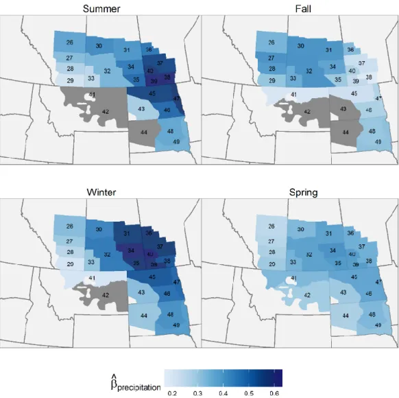
Figure 3.3 Spatial variation in the regression coefficients of local precipitation 𝑞𝑖 during the previous year on the waterfowl population size, by species and season. Shades of blue indicate positive effects of increased precipitation on population growth while shades of red indicate negative effects. Strata where 95% Credible intervals include 0 are coloured grey. ... 77
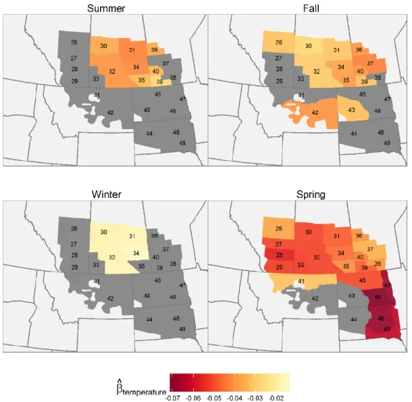
Figure 3.4 Spatial variation in the regression coefficients spring temperature (𝑞𝑖) on the waterfowl population size by species. Shades of blue indicate positive effects of maximum spring temperature on population growth while shades of red indicate negative effects. The strata which include 0 in the 95% credible interval are presented as grey. ... 78
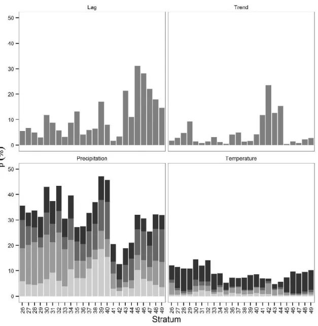
Figure 3.5 Proportions of the population variance (Eq. 3.11) explained by the different extrinsic variables.
Seasonal precipitation and temperature are stacked in top to bottom as : summer precipitation, fall
precipitation, winter precipitation, spring precipitation and spring temperature. ... 79
Figure 3.6 Pair-wise correlations (𝜌̂𝑖,𝑗) among stratum-level populations that do not include zero in their 95% Credible Intervals. The width and hue of the line represent the strength of the correlation. ... 81
Figure 4.1 a) Black Duck breeding distribution according to Nature Serve (dark grey), with breeding and
harvest area delineations used for management (vertical lines). The management zones in Canada are the Western (W), central (C), and eastern (E) breeding and harvest areas; b) Spatial grid used for prediction. Shaded cells represent the 1degree banding blocks where Black ducks were banded during at least one year over the period 1970-2010. ... 97
Figure 4.2 Temporal variation in annual band recovery probability. a) Model predictions (black line) with 95%
credible intervals (CIs; shaded area), and observed proportions of direct recoveries for juveniles (●) and adults (*). Predictions were weighted in function of the proportion of each bands type in the sample for a given year; b) Violin plots of full posterior distribution of the estimated coefficients for band type and c) other model covariates. Light grey represent juveniles while dark grey represent the adults. ... 103
Figure 4.3 Spatial predictions of recovery probabilities (left column) and the proportion of bands recovered in
Canada (right column) for juvenile Black ducks. Predicted probabilities by banding block (a,b); mean random effect for site (c,d) ; variance associated with the site effect (e,f). ... 105
xv
Figure 4.4 Temporal variation in the proportion of recoveries in Canada. a) Model predictions (black line) with
95% credible intervals (CIs; shaded area), and observed proportions of recoveries in Canada for juveniles (●) and adults (*). Predictions were weighted in function of the proportion of each bands type in the sample for a given year; b) Violin plots of full posterior distribution of the estimated coefficients for band type and c) other model covariates. Light grey represent juveniles while dark grey represent the adults. ... 106
Figure 4.5 Harvest probabilities for adult (left column) and juvenile (right column) Black Ducks. Mean derived
harvest probability distributions before the regulation changes (1982) and during the most recent hunting period (2010) (a,b); Risk Ratio between the probabilities of harvest in 2010 and 1982 (c,d); Predicted harvest probabilities (Eq. 4.9) for adult and juvenile Black Ducks for 2010 (e,f). ... 108
xvii
List of appendices
Appendix 1.1 Stan code for the Gompertz population model ... 32 Appendix 1.2 Predicted growth rate in function of the population size for the naïve model (a and c) and the
informed model (b and d). The dark grey circle present the observed growth in function of the observed populations (a and b) and the predicted growth in function of the observed population size (c and d) ... 36
Appendix 2.1 Mean and variance of the total annual rainfall and average maximum temperature as a function
of seasons for each strata between 1961 and 2010... 59
Appendix 2.2 Predicted spatial correlation function (black line) with the 95% Credible Intervals for the
intercept (K0) and the explanatory variables (KB). The dotted line represent the effective range (K = 0.05) ... 60
Appendix 3.1 Calculating priors on the intrinsic growth rate ... 86 Appendix 3.2 Stan code for the Gompertz population model ... 87 Appendix 4.1 Stan code for direct recoveries spatio-temporal model ... 114
xix
Remerciements
Au cours des dernières années, j’ai eu la chance de côtoyer plusieurs personnes qui ont de près ou de loin influencé le résultat de cette thèse. En premier lieu, j’aimerais remercier Steve Cumming, mon directeur de thèse pour m’avoir accueilli dans son laboratoire et pour son support dans la dernière ligne droite. Je veux ensuite remercier Eliot McIntire pour m’avoir fourni les bases nécessaires pour comprendre et utiliser les statistiques bayésiennes ainsi que pour plusieurs discussions stimulantes. J’ai eu la chance d’avoir François Bolduc pour m’accompagner dans mon cheminement. François a trouvé un moyen de me supporter financièrement au cours de mes études, il m’a également permis d’étendre mes horizons de recherche et a toujours été présent pour fournir un soutien moral. Je dois également remercier Stuart Slattery pour avoir essayé tant bien que mal de m’inculquer les connaissances de base pour travailler sur la sauvagine ainsi que pour avoir servi de liens avec tous les autres chercheurs du domaine. J’aimerais aussi remercier Gilles Gauthier d’avoir pris à pied levé le rôle d’examinateur interne et à Mevin Hooten pour avoir accepté le rôle d’examinateur externe.
Merci à Mélina Houle qui a toujours été là pour me prêter main-forte pour les manipulations de données et qui a également su égayer ces longs moments passés devant un écran d’ordinateur. Un grand merci à Jean-Michel Devink, Éric Reed, Jean-Dominique Lebreton, Nathan Zimpfer et Guthrie Zimmerman qui ont répondu à mes questions et qui se sont intéressés à mon projet. J'aimerais ensuite remercier tout le personnel du bureau de Québec de Canards illimités pour m'avoir accueilli parmi eux. Un merci tout spécial à Jason Beaulieu et Sylvie Picard pour leur assistance dans ArcGis. Dan McKenney et Pia Papadopol, du Service Canadien des Forêts, ont aimablement fourni les données climatiques que j’ai utilisées dans ma thèse. Je tiens également à remercier les partenaires qui m’ont supporté financièrement : Le CRSNG, le FQRNT, Canards Illimités Canada, l’Iinstitute for Wetland and Waterfowl Research ainsi que l’Association francophone pour le savoir.
Même s’ils étaient à la base de la « chaine alimentaire » plusieurs de mes collègues étudiants on eut une importance prépondérante dans mon développement intellectuel au cours des dernières années. Un grand merci à mon partenaire dans le crime numéro un : Josh Nowak. Nos sessions interminables de « whiteboard » ont probablement été parmi les moments les plus importants de mon doctorat. Merci à Sébastien Renard, avec qui j’ai partagé les joies et les peines de l’enseignement et des corrections d’examens. Je dois remercier Etienne Bellemare Racine pour son support dans R et pour m’avoir si gentiment poussé dans le rôle de président de l’association étudiante par intérim juste avant le printemps étudiant le plus chaud que l'on ait vécu depuis des décennies. Merci Étienne. Merci à Nicole Barker qui a
xx
essayé de m’enseigner tant bien que mal où l’on devrait mettre les foutus « s » dans un texte en anglais. C’était un rôle plutôt ingrat. Nicole a également eu le rôle, bien malgré elle, de m’empêcher de courir après tous ces si jolis petits “écureuils” intellectuels qu’on peut rencontrer le chemin de sa thèse et qui vous font perdre un temps fou. Merci à Jerrod Merkle qui s’est joint un peu plus tard à notre groupe, mais qui a dès le départ su apporter des idées stimulantes et une grande rigueur scientifique à nos discussions. Finalement, merci à Julien Béguin qui m’a accueilli dans le lab Cumming il y a très très longtemps et qui a toujours eu le mérite de tenir son bout dans nos discussions, ce qui évidemment a rendu nos discussions encore plus plaisantes.
J’aimerais également remercier les membres présent et passé du métalab pour les nombreuses discussions stimulantes lors de nos réunions: Émilie Allard, Yves Aubry, Sarah Bauduin, Nadia Bokenge Aridja, Aude Corbani, Stéphanie Ewen, François Fabianek, Julie Faure-Lacroix, Hermann Frouin, Pamela Garcia-Cournoyer, Marie-Hélène Hachey, Toshinori Kawaguchi, Mélanie-Louise Leblanc, Kara Lefevre, Céline Macabiau, Jean Marchal, Yosune Miquelajauregui, Ghislain Rompré, Philippe Ruiz, Frédérique Saucier, Lukas Seehausen et Maïa Sefraoui. Il ne faudrait pas oublier les étudiants de Canards illimités avec qui j’ai partagé les temps morts au bureau et des aventures sur le « terrain » ou en congrès: Stéphane Bergeron, Laurie Bisson Gauthier, Rahim Chabot, Jérome Cimon-Morin, Audrey Comptois, Geneviève Courchesne, Noémie Gagnon Lupien, Julie Labbé, Marie-Hélène Ouellet D’Amours et Aémlie Perez. Merci aussi à tous les membres de l’association étudiante pour votre dévouement et votre engagement, mais par-dessus tout pour votre bonne humeur contagieuse: Amélie Denoncourt, Édith Lachance, Louis-Vincent Gagné, Alexandre Guay-Picard, Caroline Plante, Ruth Serra, Célia Ventura-Giroux et Kaysandra Waldron.
Finalement, j’aimerais prendre le temps de remercier ma sœur Isabelle, son mari Nicholas ainsi que tous les membres des clans Boulanger et Roy pour leur patience ainsi que pour leur support et leur encouragement au cours de ces dernières années
xxi
Avant-propos
La présente thèse est composée de 4 chapitres dont je suis l’auteur principal. Chaque chapitre a été rédigé en anglais sous forme d’article scientifique. Pour chaque chapitre, j’ai établi les objectifs de recherche et formulé les hypothèses, réalisé les analyses statistiques, l’interprétation des résultats ainsi que de la rédaction de l’article scientifique.
Le premier chapitre démontre qu’il y a des lacunes importantes dans les modèles utilisés pour estimer la densité dépendance dans les séries temporelles de populations animales et comment l’utilisation de priors informatifs peut atténuer ces problèmes. L’article a été rédigé en collaboration avec Steve Cumming et Eliot McIntire et a été soumis à la revue Ecography sous le titre «Unbiasing estimates of density dependence in
time series data: a case for the use of informative priors». Le deuxième chapitre démontre l’applicabilité de la
méthode des « paramètres variables dans l’espace » pour estimer les relations non stationnaires entre les variables climatiques et l’abondance de fondrières dans la région des Prairies. Je suis le seul auteur de l’article et il a été accepté par la revue PLoS ONE sous le titre « Quantifying geographic variation in the
climatic drivers of midcontinent wetlands with a spatially varying coefficient model ». Le troisième chapitre vise
à mesurer les facteurs qui influencent la dynamique des populations de quatre espèces de canards barboteurs dans le milieu du continent et la propension des espèces à survoler la région des prairies en période de sécheresse. L’article a été rédigé en collaboration avec Eliot McIntire, Steve Cumming et Stuart Slattery et sera soumis pour publication prochainement dans une revue scientifique sous le titre « Population
synchrony of dabbling ducks in western North American». Le quatrième chapitre porte sur l’impact de la
chasse sportive sur les populations de Canards noirs sur leurs aires de reproduction au Canada. L’article a été rédigé en collaboration avec Steve Cumming et Eliot McIntire et a été accepté par la revue Ecology
and evolution sous le titre «Spatial and temporal variation in harvest probabilities for American Black Duck».
1
General Introduction
As all ecosystems on the planet experience increasing anthropogenic disturbances, there are growing concerns that our current understanding of ecological processes is too limited to design and deploy effective conservation and management strategies (Vitousek et al. 1997, Steffen et al. 2011, Barnosky et al. 2012). Our world is reportedly facing a ‘toxic cocktail’ of anthropogenic disturbance and climate change, and there is a widespread belief that climate change will only exacerbate the negative effects of anthropogenic disturbance on many species (Travis 2003, Brook et al. 2008). Conservation programs and population management are however clouded by uncertainty since our understanding of the dynamics and conditions of resources affecting populations are incomplete and because the ecological systems are inherently stochastic (Williams and Johnson 2013). In response to this uncertainty, there has been a concerted effort to move from phenomenological approaches (i.e., correlative models) to process-based models (i.e., mechanistic models) that incorporate realistic amounts of complexity to deepen our understanding of ecological systems (Evans 2012, Evans et al. 2012). These process-based modelling exercise are intended to generate a solid understanding of how environmental changes at the global scale can lead to changes in animal populations down at the individual scale (Chave 2013). The overall theme of this thesis is to develop spatially explicit model to assess the variation in the drivers of dabbling ducks populations in North America and asses the importance of this variability.
Dabbling duck ecology
The primary breeding habitat of many dabbling species is concentrated in the Prairie Pothole Region (PPR) but the breeding ranges of many species also extend to the Boreal Forest and the Canadian Arctic (Bellrose 1976, Johnsgard 2010). As with many species, there are currently a host of challenges for the conservation and management of dabbling duck populations due to anthropogenic disturbance and these challenges vary substantially as a function of the region concerned (Nichols and Williams 2006, Slattery et al. 2011). Wetlands in the PPR are highly productive, which make them attractive to waterfowl, but they are also highly dependent on precipitation for their water supply (Covich et al. 1997, Murkin et al. 1997, Euliss et al. 2004). This dependence on climatic conditions induces a cycle of wetness and drought that is one of the defining features of the pothole region (Millett et al. 2009). These characteristics also make PPR wetlands particularly vulnerable to climate change. It is currently predicted that the western PPR will get drier over the 21st century
while the eastern PPR will get wetter (Johnson et al. 2005, 2010). This would be detrimental to waterfowl populations because the best breeding habitat is situated in the western PPR (Johnson and Grier 1988, Johnson et al. 2005, 2010). Should the precipitation regime be altered by climate change, the productivity of
2
the wetland could also be altered, ultimately affecting the productivity of the waterfowl populations nesting in the region (Walker et al. 2013).
The PPR drought cycle is not synchronized across the whole region and some authors have speculated that the size of waterfowl populations track the variation in climate and wetness (Johnson and Grier 1988, Johnson et al. 2005, 2010). During more severe droughts, some species such as the Northern Pintails are believed to “overfly” the drier Prairies and settle further north in the Boreal Forest (Smith 1970, Calverley and Boag 1977, Hestbeck 1995). Some authors have also suggested the reverse, whereby populations in the Boreal may be lower than average during exceptionally good years in the PPR, due to “short stopping” (Hansen and McKnight 1964). A change in hydrological regime could also change the spatial structure of the populations. Finally, In the United States, the conservation Programs that have been used to protect and enhance PPR wetlands are currently being challenged. Some conservation program are also under revision and there are no guarantees that PPR wetlands will benefit from the same extensive protection in the future (Haukos and Smith 2003, Van Der Valk and Pederson 2003, Rashford et al. 2011). The wetlands conservation programs have also failed to keep pace with rising values of agricultural commodities in the US (Rashford et al. 2011).
The picture is even murkier outside of the PPR. Although there is a rich history of studying demographic rates and habitat selection for waterfowl populations in the PPR, the populations in the Boreal Forest are still poorly documented (Slattery et al. 2011). Yet many species of diving ducks reach their highest densities in the Boreal Forest and about 29% of the total waterfowl population breed in this biome each year (Sénéchal 2003, Lemelin et al. 2010, Slattery et al. 2011). Dabbling species such as the Black Duck (Anas rubripes) and the Green-winged Teal (Anas crecca) are also closely associated with the Boreal Forest (Johnson 1995, Longcore et al. 2000b). The importance of Boreal populations have been over-looked for a long time ,in part, because the Boreal Forest has been seen as a remote and virgin environment free of human disturbances (Lynch 1984, North American Waterfowl Management Plan 2004, Slattery et al. 2011). However, there are now a plethora of anthropogenic activities in the Boreal Forest that can negatively affect biodiversity even at high latitude(Schindler and Lee 2010). The conservation opportunities diminish rapidly as the Boreal Forest is affected by forestry, oil and gas exploration, hydroelectric development, and mining(Foote and Krogman 2006, Schindler and Lee 2010). There is currently little demographic information on bird populations in the Boreal Forest and these knowledge limitations hamper our capacity to assess how populations might react to habitat and climate change (Niemi et al. 1998, Schmiegelow and Mönkkönen 2002)
Waterfowl management
Many species of waterfowl are intensively harvested for food and sport. Conservation and management actions for harvested species aim at preserving populations at levels that permit a sustainable use (Williams et
3 al. 2002, Organ et al. 2012).There are currently two major programs concerned with managing North American waterfowl populations to sustainable levels. The first main conservation program is the Adaptive Harvest Management (AHM) framework and is mainly concerned with setting hunting regulations within the United States. The AHM was implemented as a “systematic approach for improving resource management by learning from management outcomes” (Williams et al. 2002). The United States Fish and Wildlife Service, the Canadian Wildlife Service, and various state, provincial and private partners carry out many monitoring population program (Nichols et al. 1995a), however the AHM program relies on two main sources of information to achieve its objectives: extensive population monitoring, and banding programs. The Waterfowl Breeding Population and Habitat Survey which is conducted in May over the most important breeding grounds in the mid-continent and in the east of the continent (Smith 1995, Zimmerman et al. 2012). This systematic survey provides annual estimates of the breeding population size for many species of ducks (Nichols 1991a, Smith 1995). Large scale banding programs have also been implemented to estimates annual survival and harvest rates (Nichols et al. 1995a, Nichols and Williams 2006). Although these dataset represent a unique opportunity for the analysis of population dynamics, these monitoring programs were designed specifically to inform harvest decisions at the continental and flyway scale (Nichols et al. 2007) and present specific challenges for all alternate uses.
The second major conservation program is the North American Waterfowl Management Plan (NAWMP) which is an international partnership that aim at fostering the conservation and protection of wetlands associated with waterfowl in North America. Both major conservation programs have evolved somewhat separately and are infused with a different culture (Runge et al. 2006). Harvest management is centralized and is mainly driven by US authorities while the NAWMP is fundamentally de-centralized, characterized by a plurality of public and private actors, and is concerned in great part by the state of the breeding habitat on the Canadian breeding grounds (Johnson 2011). It was recognized early in both programs that successful management of continental waterfowl populations would depend on the development of ecological knowledge. However, the programs have evolved somewhat independently and due to their different setting, goals, and actors the two programs are sometimes at odds (Runge et al. 2006, Johnson 2011). Particularly problematic are the population goals of the NAWMP that aim at maintaining the population at the levels observed during the 1970’s. These population objectives, do not take account the harvest context and the impact of environmental factors that are affecting population dynamics (Runge et al. 2006, Anderson et al. 2007, Johnson 2011). The lack of cohesion between the two programs is becoming more evident as they move in opposite directions within their respective scale of operation. The management of the continental populations, a top-down management process, is being scaled down increasingly and more information is being made available about the metapopulation dynamics of waterfowl (Esler 2000, Mattsson et al. 2012). Meanwhile the wildlife habitat program, which is a bottom up management process, is being scaled up from local effort to landscape and regional conservation program
4
(Abraham et al. 2007). As the objectives of both programs are being refined there is a clear need for a better integration of programs relating to population and habitat (Runge et al. 2006, Johnson 2011) and there has been a call for the development of an integrated modeling framework for making simultaneous predictions about the effects of harvest and habitat management (Anderson et al. 2007).
Population dynamics
For many years, the emphasis in conservation biology has been on identifying, prioritizing, and managing targeted species’s habitats (Mace et al. 2010). However, conservation priorities have evolved over time and there is now a general acknowledgement that population dynamics are as equally important to address when conserving species (Keith et al. 2008, Mace et al. 2010, Fordham et al. 2013). For migratory birds such as dabbling ducks, current efforts are now directed to a developing, more holistic view, encompassing not just the breeding grounds but also migration routes and wintering ground conditions, both of which can significantly affect the success of conservation programs (Sherry and Holmes 1996, Faaborg et al. 2010). There is also a widespread acknowledgement that understanding population structure is critical to developing effective conservation approaches, both as a tool to define management units but also to identify the demographic constraints that regulate populations (Esler 2000). This shift in research priorities is also reflected in the in the waterfowl management world; it has become evident that traditional approaches to wildlife habitat programs (e.g., land purchase, wetland management) will not be sufficient to meet management objectives (Abraham et al. 2007) and efforts are now being redirected at landscape and regional population management. For exploited species that are widely distributed, it is now readily acknowledged that management strategies require accurate knowledge of landscape conditions, detailed information on species metapopulations, demographic rates, and an understanding of how discrete breeding populations are affected by regional harvest (Runge et al. 2006, Mattsson et al. 2012). For waterfowl species in particular, it has proven difficult to scale up the effects of local conservation effors to continental populations. As a consequence, the examination of population dynamics at regional levels might be a more tractable approach to gauge current management efforts (Abraham et al. 2007).
Change in population size are driven by four fundamental demographic processes: birth, survival, immigration, and emigration (Nichols 1991b, Perrins 1991, Williams et al. 2002). Factors affecting the demographic parameters of a population can themselves be grouped in two broad families: extrinsic factors and intrinsic factors (Williams et al. 2002). Extrinsic factors include resource availability, generalist predators, climate, and weather while intrinsic factors are mainly concerned with the effects of population density on the population demographic rates (Newton 1991, Pasinelli et al. 2011). For this reason, the factors affecting populations have often grouped into density independent (extrinsic) and density dependent (intrinsic) factors. While any process that affects population dynamics will be a limiting factor, only an intrinsic factor can regulate the population
5 (Sinclair 1989).This distinction has led to contentious debates in ecology to determine if populations are limited by their environment or regulated by their own density dependent feedback mechanisms (Andrewartha and Birch 1954, Nicholson 1954, Berryman et al. 2002, White 2008).
Because of the inherent difficulties in measuring density dependence and identifying the mechanisms responsible for it, some have suggested to do away with the concept and focus on the factors limiting populations at the local scale (Wolda 1989, White 2008). However, without density dependence there is no need for conservation as the animals should be able to move out of degraded habitat and crowd the best habitat available without any negative consequences (Sutherland and Norris 2002). In the case of harvested species, absence of density dependence also means that any removed individual is a net loss that cannot be replaced, so that fixed rates of exploitation inexorably leads to extinction (Anderson and Burnham 1976, Lebreton 2005). The concept of density dependence therefore remains central for both conservation and management even if it is sometimes obscured. The current consensus is that populations are both limited by their environment and regulated by density feedback mechanisms, but that the contribution of each process varies over time or space (Bjørnstad and Grenfell 2001, Stenseth et al. 2003). If they can be identified, the form and strength of density dependence in a population should shape the relevant conservation and management actions (Henle et al. 2004, Runge et al. 2006). Research efforts should therefore be directed at teasing apart the effects of each process and identifying their respective contribution to achieve efficient conservation and management strategies (Coulson et al. 2000, Colchero et al. 2009).
Within a species geographic range, there will be a network of subpopulations connected by dispersing individuals. Species populations therefore possess a spatial structure (Pulliam 1988, Ritchie 1997, Goodwin and Fahrig 1998) which can be as important in population dynamics as the fundamental demographics of each individual population (Dunning et al. 1992, Hanski 1998). Population dynamics thus necessarily occur in a spatial context (Ricklefs 1987, Kareiva et al. 1990). Managing local populations is often complicated by the great difficulty in establishing the limits of a population (Berryman and Kindlmann 2008). Moreover, the respective contribution of intrinsic and extrinsic factors can change throughout the species’ range (Royama 1992, Williams et al. 2002). The spatial variability, whether it is in the environmental drivers or within the population itself , can be substantial and managers need to acknowledge this variability and account for it in the implementation on their management actions (Shea 1998).
Spatial hierarchical models
The desire to develop more mechanistic models of spatial population dynamics has led to a surge of “hierarchical” models in ecology (Mackey and Lindenmayer 2001, Royle and Dorazio 2008, Cressie et al. 2009, Halstead et al. 2012). Hierarchical models allow the user to decompose the observed data into a
6
sequence of simpler probabilistic models that are linked together (Wikle et al. 1998, Wikle 2003, McCarthy 2007). They provide a framework to explore the structure of parameters within the model (Sauer and Link 2002, Link and Barker 2009) and allow for the possibility of taking observation error into account within the model structure (Cressie et al. 2009, Ponciano et al. 2009). One of their most powerful features is the ability to combine datasets together to “shrink” the estimates of the individual parameters. That is, by imposing a hierarchy among the dataset, via a random effect, it is possible to “borrow strength for the ensemble” and get better estimates than one would get by estimating for the component datasets independently (Gelman and Pardoe 2006, Gelman and Hill 2007, Kéry and Schaub 2011). Hierarchical models can also directly incorporate spatial dependency at multiple scales (Wikle et al. 1998, Clark 2007, Cressie and Wikle 2011), which is an important challenge in ecology (Levin 1992, 2000, Noda 2004, McMahon and Diez 2007).
Analysis of spatially dependent data is complicated by the fact that assumption of independent errors are often violated(Fortin and Dale 2005). Spatial autocorrelation reflects the axiom that things that are close together are more related than things that are distant. Making inference on data that is thought to be independent, when they are actually correlated, will lead to erroneous inference as the estimated variance will be too small (Cressie and Wikle 2011). Significant efforts have been made in recent decades to develop quantitative methods that can account for spatial autocorrelation (Banerjee et al. 2004, Fortin and Dale 2005, Gelfand et al. 2006, Dormann et al. 2007). Spatial autocorrelation is now generally accommodated by adding a spatial random effect to the mean (Finley 2011, Fortin et al. 2012, Jarzyna et al. 2014).
Most current spatial models, however, assume that the underlying processes are stationary (Fortin and Dale 2005, Finley 2011, Jarzyna et al. 2014), that is to say that the relationship between the response variable and the explanatory variable is expected to be stable though space. However, the strength and the nature of the relationship between predictor and the response variables can vary across large spatial domains, such as between the PPR and the WBF inducing spatial stationarity (Fortin et al. 2012, Miller 2012).This non-stationarity can be due to unobserved interactions or the presence of inherently different mechanisms (Miller 2012). For data collected and modeled across large-scale spatial domains it can therefore be unrealistic to assume that single set of set of regression coefficients will adequately capture the relationship between the predictor and response variables (Finley 2011, Winiarski et al. 2013, Jarzyna et al. 2014). In the ecological literature, non-stationary relationships are especially prevalent for climatic data such as temperature and precipitation (Foody 2004, Grøtan et al. 2009a, Jarzyna et al. 2014) as the relationship between climate and species is often indirect. Despite the importance of this problem, has generally been overlooked in ecology but also in statistics. In recent years, geographically weighted models (GWR) have become increasingly popular to deal with this issue (Fotheringham et al. 2003). A major drawback of GWR are that a regression is fitted for each sampling location, making generalization difficult (Fortin et al. 2012). In contrast, Bayesian
spatially-7 varying coefficient (SVC) models use a multivariate spatial process instead of fitting spatially local regression models (Gelfand et al. 2003, Wheeler and Calder 2007). The SVC approach thus fits naturally within a hierarchical context. This approach could therefore be highly relevant in ecology as it is mostly concerned with the variations in the abundance, diversity, or metabolic activity of organisms through time and space and the cause and consequence of these variations (Currie 2007, Krebs 2009). The application of the SVC approach would be particularly interesting in the context of dabbling ducks population dynamics since the populations limiting factors are thought to vary significantly throughout the range of many species (Grøtan et al. 2009b, Mcnew et al. 2013).
Methodological approach
The main objective of my thesis was to quantify the spatial variation in duck populations of North America, determine the importance of this spatial variation and identify the key factors that may influence it. I used two main axes of research to approach this problem. The first axis aimed at characterizing the relative importance of intrinsic and extrinsic factors in the dabbler populations of the Mid-continent and in the spatial variation associated with those factors. This work relied on analysis of duck counts from the Waterfowl Breeding Population and Habitat Survey. The second axis of research aimed at quantifying the role of harvest in dabbling populations; for this, I used data form the annual banding program
For the first axis of research, my primary task was to develop spatially explicit population models for several species to assess the respective contribution of the intrinsic and extrinsic factors in the population dynamics of dabblers and how their respective contributions vary regionally. There are some important pitfalls associated with the use of population models based on time-series (Dennis et al. 2006, Knape 2008, Clark et al. 2010). Notably the density-dependent term and the intrinsic growth rate are not identifiable and this problem can lead to spurious results, such as biologically impossible reproductive rates (Lillegard et al. 2008, Delean et al. 2013, Lebreton and Gimenez 2013).
In Chapter 1, I introduce a spatially explicit population model to determine the respective contribution of intrinsic and extrinsic factors on population growth of Mallard (Anas platyrhynchos) populations. I show how some of the pitfalls associated with population models can be avoided with the use of informative priors on the intrinsic growth rate. I used the Mallard population data to form the Waterfowl Breeding Population and Habitat Survey and for extrinsic environmental factors I used total precipitation during the year preceding each survey , mean spring daily maximum temperature as both of these factors had been demonstrated to play an important role in the ecology of the Mallard in the mid-continent population (Johnson and Grier 1988, Larson 1995, Miller 2000).
8
In Chapter 2, I assessed the dynamics of wetlands abundance in the PPR. Although the amount of total precipitations is a good indicator of wetland conditions in the Prairie-Pothole Region (Larson 1995, Withey and van Kooten 2011, Niemuth et al. 2014) there has been no integrated model assessing how these ecological drivers vary spatially. To fill this knowledge gap I used the spatially varying coefficient approach to quantity the spatial variation in the main drivers of wetland abundance in the Prairie-Pothole region. I used an auto-regressive model where the abundance of wetlands is correlated with the abundance of wetlands during the previous year, the amount of seasonal precipitation during the previous year and the mean maximum temperature during each season. The results of this chapter demonstrate that winter and fall precipitation are the most important climatic drivers but their respective contribution in wetlands dynamic varied spatially. Pond density in east of the survey area was more dependent on the temporal autoregressive term (e.g., lagged pond abundance) than on lagged precipitation. My results also suggest that the role of lagged summer precipitation has been overlooked in the published accounts of wetlands dynamic for the region.
In Chapter 3 (Overflight) I extended the population model developed in Chapter 1 to assess the importance of ‘”overflight” in the dynamics of four species of dabblers. Because they are migratory, dabbling ducks can demonstrate flexibility in their choice of nesting habitat (Johnson and Grier 1988). Since the PPR is subject to a cycle of drought it has been theorized that some individuals could overfly the PPR and take refuge in the WBF (Crissey 1969, Johnson and Grier 1988, Hestbeck 1995). For this chapter I focused on Mallards, Northern Pintails (Anas acuta), American Wigeons (Anas americana) and Green-winged Teals since these species are widespread in the survey area, and yet have distinct ecological niches and propensities to “overfly” the PPR. I also used a more refined approach for the extrinsic climatic factors based on the results of the second chapter. This approach allowed me to capture important variation in the population dynamics of the four species. The results of this chapter demonstrated that the species that most sensitive to the extrinsic factors are the species that are the more prone to “overflight.” Using lagged seasonal precipitation instead of lagged total annual precipitation demonstrated the importance of summer precipitation during the previous year for the population of all four species. These results suggest that wetland persistence during summer play an important role in the population growth of all four species
In Chapter 4, I use similar statistical approached applied to a more directly management focussed problem. I sought to measure the temporal and spatial variation in harvest rate of American Black Duck populations. Harvesting pressure can be an important factor in population dynamics(Anderson and Burnham 1976, Williams et al. 2002, Lebreton 2005). The analysis of harvest in the mid-continent dabbler populations is however complicated by the use of different flyways by the different populations and the varying reporting rates among flyways and jurisdictions (Boomer et al. 2013). I therefore used the Black Duck in eastern Canada as a reference case as the migratory patterns of the species are less complicated. Moreover, the Black Duck is a
9 species of concern in North-America since its populations declined markedly between the 1950’s and 1990’s (Geis et al. 1971, Longcore et al. 2000b, Devers and Collins 2011). Harvest rates are typically derived from recovery and reporting probabilities from bands analysis (Brownie et al. 1985). However, estimating harvesting probabilities from banding data can be challenging since reporting and recovery probabilities can have distinct spatial patterns. To assess the fine scale spatial variability in harvest probabilities I developed hierarchical logistic regression models with spatially correlated errors on a 1 degree grid. I evaluated the probabilities of band recovery and the proportion of individual harvested in Canada via the spatially explicit logistic regressions. I subsequently derived the probability of harvest from these values, in combination with independent estimates of reporting probabilities in Canada and the USA derived from Garrettson et al. (2013). My results show that the harvest probabilities were correlated with the hunter effort but did not decrease after the implementation of new, stricter, harvest regulations. There is also fine scale variation in harvest probabilities for Black Duck on the Canadian breeding ground and the harvest probabilities should be closely monitored along the Saint Lawrence River system and in the Atlantic to avoid over-exploitation.
All chapters of this thesis address the importance of spatial variation and characterize its importance in population dynamics. In the conclusion, the link between each chapter and the adaptive management of waterfowl population will be addressed. Finally, the implications and future outcome of the results presented in this thesis will be discussed.
11
Chapter 1
Unbiasing estimates of density dependence in time
series data: a case for the use of informative priors
12
Abstract
While there is mounting evidence that the factors regulating population dynamics can be variable across species range most population models are assuming that population parameters are stationary. We therefore developed a spatially explicit Gompertz population model to assess the variation in the intrinsic growth rate (r), density dependence (β) and extrinsic populations drivers and used we used spatially stratified time series population estimates of the Mallard (Anas platyrhynchos) as a case study for our model. We included the effect of precipitation during the previous year and spring maximum temperature in the current year as extrinsic drivers in the model. Because density dependent models can give biased answers for time series abundance data we fitted a naïve model without informative priors and a model where we constrained the mean and variance of r to biologically realistic values that were derived from a comparative demography approach. In the naïve model r and β were not identifiable and the model overestimated their values leading to unrealistic population growth. The naïve model also produced significant differences between the population r and return time to equilibrium (1⁄-β) across the survey area. In contrast, in the informative model, the intrinsic growth rate and the return time to equilibrium term were generally equal across populations. The return time to equilibrium in the informative model were also longer than in in naïve model, and indeed were longer than the wet-dry cycle in some parts of the Prairie- pothole region. The effect of the extrinsic climatic factors were however similar across models. Population growth in the Prairies-Pothole Region is driven in large part by precipitation while spring temperature limits the populations growth in Alaska. Our results that even under the best case density dependent models for time series can have identifiability issues and should be approached with care.
Keywords: demographic models, density dependence, environmental stochasticity, Gompertz population
13
Résumé
Bien qu’il soit reconnu que les facteurs qui régulent la dynamique des populations soient variables à l’intérieur de l’aire de distribution d’une espèce, la plupart des modèles de populations assument que les paramètres intrinsèques de la population sont stationnaires. Nous avons en conséquence développé un modèle de population Gompertz explicitement spatial pour mesurer la variation spatiale dans les taux de croissance intrinsèques, la force de la densité dépendance, ainsi que les effets des facteurs extrinsèques de différentes populations. Nous avons utilisé des séries chronologiques de populations de Canards colverts (Anas
platyrhynchos) stratifiés spatialement pour tester le modèle. Nous avons inclus l’effet des précipitations durant
l’année précédente et la température maximale moyenne durant le printemps de l’année d’inventaire comme facteurs extrinsèques dans le modèle. Les modèles de densité dépendance peuvent produire des résultats biaisés, et afin de contrôler pour ce type de biais, nous avons comparé deux modèles. Nous avons comparé un modèle naïf, sans information à priori, et un modèle où nous avons fixé la moyenne et la variance du taux d’accroissement intrinsèque à des valeurs biologiquement réalistes à l’aide d’une approche comparative de la démographie. Pour le modèle naïf, r et β n’étaient pas uniquement identifiable et le modèle a surestimé les valeurs des deux paramètres. Les résultats du modèle « naïf » indiquent que r et β ne sont pas identifiables individuellement et qu’en conséquence, le modèle surestime grossièrement le taux d’accroissement de la population. Le modèle « naïf » a également produit des différences significatives entre les taux de croissance intrinsèques des populations ainsi que dans les temps de retour à l’équilibre après perturbations (1 −𝛽⁄ ) des différentes populations. Par contre, les résultats du modèle avec des informations à priori montrent que les taux intrinsèques d’accroissement des populations et les temps de retour à l’équilibre n’étaient pas significativement différents entre les populations. Les temps de retour à l’équilibre dans le modèle des informations à priori étaient plus longs que dans le modèle « naïf » et même plus longs que le cycle de sécheresse dans certaines parties de la région des fondrières des prairies. Les résultats pour les facteurs extrinsèques étaient toutefois comparables entre les deux modèles. Les populations de la région des fondrières des prairies sont en grande partie limitées par les précipitations durant l’année précédente tandis que les populations de l’Alaska et de la région de Mackenzie sont limitées par la température durant le printemps. Nos résultats se joignent à un nombre croissant de preuves indiquant que les modèles de densités dépendance pour les séries temporelles peuvent produire des résultats biaisés si le taux de croissance intrinsèque n’est pas contraint à des valeurs qui sont biologiquement réaliste. Bien que ces résultats n'influencent pas l’estimation des paramètres extrinsèques, les modèles qui ne présentent pas les valeurs estimées de croissance intrinsèques devraient être examinés avec soin.
Mots-clés: densité dépendance, modèles démographiques, modèle de population Gompertz, modèles
14
Introduction
Density dependence is often measured at the population level even though the process is related to individual resource availability and performance; this has led to numerous difficulties and controversies (Murdoch 1994, Lebreton 2009). While few now question the existence of density dependence per se (but see White 2008) the key question is whether the intrinsic, biological factors that cause it are important in comparison to other sources of variation in population size (Ives et al. 2003). The key drivers of population dynamics are not always evident and the relative importance of extrinsic factors, such as weather, has been much debated (Bjørnstad and Grenfell 2001, Stenseth et al. 2003). The current agreement is that both intrinsic and extrinsic factors are important for understanding population fluctuations and the emphasis should be put on quantifying the complex interplay between them (Bjørnstad and Grenfell 2001, Stenseth et al. 2003, Ross 2014).
A major hurdle however is that the relative importance of intrinsic and extrinsic factors can vary geographically (Williams et al. 2003, Saether et al. 2008). At large extents, spatial gradients in density dependence have already been demonstrated for ungulates and small mammals with southern populations being more strongly regulated by population feedback than are northern populations, where climatic factors override effects of intraspecific competition (Bjørnstad et al. 1995, Post 2005, Wang et al. 2006). Variation in demographic parameters has also been demonstrated at smaller scales, where landscape heterogeneity has been demonstrated to affect the manner in which animals exploit available resources (Shima and Osenberg 2003, Sibly et al. 2009). Identifying the spatial variation in the drivers of population dynamics can therefore play an important role in the conservation and management of exploited species (Williams et al. 2002), and failing to account for his variation can lead to biased estimates of demographic parameters. The spatial variation in the density dependent process has, however, received limited attention and while recent development in the field allows spatial variation to be estimated in the intrinsic growth rate of the population (Thorson et al. 2014), no models that deal explicitly with spatial variation in density dependent processes and extrinsic drivers have been proposed.
The problem of analysing density dependence is compounded by the limitations imposed by the tools and data that are available. Non-identifiability of parameters in the models used to analyse population time-series poses a major challenge (Lillegard et al. 2008, Clark et al. 2010, Lebreton and Gimenez 2013). Intrinsic growth rate and the density dependent term cannot be estimated separately in classic density dependent models. When fitted with only abundance data, these models tend to have positively biased and ecologically unrealistic estimates of the intrinsic growth rates and, in consequence, to overestimate the strength of density dependence (Polansky et al. 2009, Clark et al. 2010, Lebreton and Gimenez 2013). Recent developments have suggested controlling for observation error via repeated sampling, or resampling of the available data, or including more ecological realism such as extrinsic explanatory variables accounting for spatial variation might
15 alleviate some of the problem, but these solutions have been applied to a limited number of real datasets. A more direct solution that has been suggested is to use a Bayesian approach with informative priors on the intrinsic growth term (Delean et al. 2013, Lebreton and Gimenez 2013). In this instance, an informative prior on growth rate can be derived by the comparative demography approach or from allometry (Niel and Lebreton 2005, Delean et al. 2013)
In this paper we fill a gap in the analysis of density dependent process by introducing a spatially explicit version of the Gompertz model based on the spatially-varying coefficients method and we assess the impact of using informative priors on the conclusions drawn from the model. We used Mallard (Anas platyrhynchos) data from mid-continental North America. Mallard reproductive output is thought to be higher in the south of its breeding range while Mallard survival is thought to increase in northern latitudes (Calverley and Boag 1977, Hestbeck 1990, Hestbeck et al. 1992). Density dependence has been demonstrated at several life stages of Mallard, but is thought to act particularly during the breeding season (Kaminski and Gluesing 1987, Elmberg et al. 2005, Gunnarsson et al. 2006). Extrinsic factors have also been demonstrated to be important in part of the breeding range of the Mallard. Mallard population growth rates vary markedly with wet-dry fluctuations in the Prairie pothole region (Drilling et al. 2002, Viljugrein et al. 2005, Saether et al. 2008). The impact of climatic factors are less clear for northern population, but spring temperature is thought to be limiting recruitment (Miller 2000, Drilling et al. 2002).
Our main objective was to estimate extrinsic and intrinsic effects on population dynamics of a wide-ranging species. To do this, we felt that the possible bias in the estimation of intrinsic factors from time series data would affect the estimation of the intrinsic factors, and might also affect the estimation of the extrinsic factors. We hypothesized that informative priors are required to estimate biologically reasonable, spatially varying values for the intrinsic growth rate and density dependence even when accounting for observation error and including extrinsic covariates. To test this hypothesis we fitted a naïve model without informative priors and a model where informative priors on the intrinsic growth were estimated by comparative demography. We further hypothesised that a model without informative priors would overestimate both the intrinsic growth rate and the strength of density dependence because of non-identifiability. The uncertainty in the estimation of these values should also amplify the differences among populations leading to inaccurate conclusion in regard to the spatial variability of the intrinsic factors. The model with the informative prior is expected to produce more ecologically reasonable results but should also diminish the spatial differences because of the constraints on the model. We also assessed if the estimated effects of extrinsic variables were affected by the use of the informative prior. Our expectation was that the identifiability issue would not affect these estimates and that consequently the results on extrinsic factors would be similar in the two models.
16
Methods
Population data
Annual duck counts were obtained from the Waterfowl Breeding Population and Habitat Survey (WBPHS), conducted annually by the US Fish and Wildlife Service (USFWS) and Canadian Wildlife Service (CWS; Figure 1.1). This aerial survey has been conducted since 1955 over major waterfowl breeding areas in Canada and the United States (Smith 1995). The WBPHS is one of the longest running and most spatially-extensive wildlife survey in the world (Williams et al. 2002, Nichols and Williams 2006) so it is a good candidate to address the strengths and limitations of analyses using time series data. Spatial variation in duck distribution is addressed through systematic stratified sampling (Figure 1.1). Within strata, line transects of variable length are flown by a fixed-wing aircraft approximately 50 m above ground level. Two observer record all waterfowl seen within 200m each side of the flight line. The counts are corrected for detection error using visibility correction factors derived from historical helicopter surveys or annual ground surveys that occur concurrently on a subsample of the aerial survey transects (Smith 1995). Stratum level population estimates are subsequently derived from the visually corrected counts. We used the strata population estimates from 51 survey strata in the Prairie Pothole Region (PPR) and the Western Boreal forest (WBF). We grouped the strata into sub-regions adapted from Boyd (1991) for descriptive purposes but did not use these sub-regions in the analysis. We used annual strata level counts from 1961 through 2010 to ensure overlap between population and climate data.
17
Figure 1.1 Study area and strata (n=51) used for the analysis. Shading represents waterfowl
sub-regions adapted from Boyd (1991). Numbers indicate strata numbers.
Climatic data
We included total precipitation during the previous year and the mean daily maximum temperature during the spring as an explanatory variable in the population model. The amount of wetlands presents in the PPR can be largely explained by the amount of precipitation during the previous year (Larson 1995, Niemuth et al. 2014). Wetlands abundance, has been demonstrated to affect positively the size of Mallard populations in this region (Johnson and Grier 1988, Viljugrein et al. 2005). Spring temperature has also been demonstrated to decrease the numbers of wetlands in the PPR particularly in the eastern part (Larson 1995, Niemuth et al. 2014). It is largely thought that wetlands in the WBF are more stable and thus do not impact waterfowl population dynamics in the WBF (Nudds 1983, Lynch 1984). However, there has never been any formal testing of this hypothesis to our knowledge. There is some empirical data to support that assertion however as the wetlands wet-dry cycle is considerably longer and less pronounced in the WBF than in the PPR (Ferone and Devito 2004, Price et al. 2005). Low spring temperature has also been suggested as a limiting factor for the Mallard population in the WBF but the evidence regarding this hypothesis is limited as well (Miller 2000).
Given these hypotheses, we expect the total precipitation during the previous year to have a strong positive effect on Mallard abundance in the PPR and we expect the positive effect of precipitation to decrease as we move northward from the PPR, through the Parklands and into the boreal forest. We expect the opposite pattern for temperature. In other words, temperature should have negative effect on the breeding population