Science Arts & Métiers (SAM)
is an open access repository that collects the work of Arts et Métiers Institute of Technology researchers and makes it freely available over the web where possible.
This is an author-deposited version published in: https://sam.ensam.eu
Handle ID: .http://hdl.handle.net/10985/19295
To cite this version :
Alberto BADÍAS, David GONZÁLEZ, Icíar ALFARO, Francisco CHINESTA, Elías CUETO - Real time interaction of virtual and physical objects in mixed reality applications - International Journal for Numerical Methods in Engineering - Vol. 121, n°17, p.3849-3868 - 2020
Any correspondence concerning this service should be sent to the repository Administrator : archiveouverte@ensam.eu
Real-time interaction of virtual and physical objects in
mixed reality applications
Alberto Badías
1David González
1Icíar Alfaro
1Francisco Chinesta
2Elías Cueto
11Aragon Institute of Engineering Research, Universidad de Zaragoza, Zaragoza, Spain
2ESI Group Chair @ PIMM - Procédés et Ingénierie en Mécanique et Matériaux, ENSAM ParisTech, Paris, France
Correspondence
Elías Cueto, Aragon Institute of Engineering Research, Universidad de Zaragoza, Edificio Betancourt. Maria de Luna, s.n., Zaragoza 50018, Spain. Email: ecueto@unizar.es
Funding information
Ministerio de Ciencia e Innovación, Grant/Award Number:
CICYT-DPI2017-85139-C2-1-R
Summary
We present a real-time method for computing the mechanical interaction between real and virtual objects in an augmented reality environment. Using model order reduction methods we are able to estimate the physical behavior of deformable objects in real time, with the precision of a high-fidelity solver but working at the speed of a video sequence. We merge tools of machine learning, computer vision, and computer graphics in a single application to describe the behavior of deformable virtual objects allowing the user to interact with them in a natural way. Three examples are provided to test the performance of the method.
K E Y W O R D S
model order reduction, nonlinear materials, real-time interaction, solids contact
1
I N T RO D U CT I O N
New technologies are bringing better tools to improve the augmented and mixed reality experience. These tools are in the form of both hardware and software. On the hardware side we have the development of new devices to show information to the user, such as smartphones, or high-resolution virtual reality glasses (eg, StereoLabs ZED Mini on Oculus Rift, see https://www.stereolabs.com/zed-mini/setup/rift/); we also notice great efforts on the development of devices to capture information around us such as RGB-D systems (Microsoft Kinect for Windows, for instance, see https:// developer.microsoft.com/en-us/windows/kinect), or stereo cameras; and even systems that include both the capture and visualization of information, such as Microsoft Hololens 2 (https://www.microsoft.com/en-us/hololens) or Magic Leap
One(see https://www.magicleap.com/magic-leap-one), which allow the capture of the environment, the visualization of virtual objects and the interaction thanks to built-in controls.
From the software point of view, a great work has been done to generate new environments to reduce complexity in the process of capturing the data, such as the new development kits Apple ARKit 3 (https://developer.apple.com/augmented-reality/) or Google ARCore (https://developers.google.com/ar/); other software development kits are more focused and integrated into helmets such as Hololens; there are also great advances in visualization libraries such as OpenGL (https:// www.opengl.org/) or other proprietary libraries like Nvidia CUDA (https://developer.nvidia.com/cuda-zone) or Apple
Metal(https://developer.apple.com/metal/); and also there has been a big development in new techniques to take robust measures from a scene, such as ORB-SLAM1or LSD-SLAM,2among others.
This paper leverages some of these technologies and develops real-time computational mechanics techniques so as to provide mixed reality systems the ability to seamlessly integrate virtual and physical objects and make them interact
F I G U R E 1 Mixed Reality (MR) as the interaction of three sciences: machine learning, computer graphics, and computer vision [Color figure can be viewed at wileyonlinelibrary.com]
according to physical laws. The interest of adding physical realism to the interaction between real and virtual elements in a scene is to increase the degree of perceived realism for the user. In other words, the degree of presence in the mixed envi-ronment. The addition of physical behavior to this interaction is something not yet explored, to our knowledge, in previous augmented/mixed reality (AR/MR) applications. The degree of perceived realism is expected to increase substantially in this type of applications, and this makes it worth exploring the ways to do it.
We believe that this fusion is novel in the field of mixed/augmented reality and has not been applied in current systems, where augmented reality is understood as the positioning of static information in space3or animated sequences,4 but
in very few cases deformable solids are taken into account.5We are looking for a simple and natural interaction with
virtual objects, which are capable of deform as if they were really in front of the user. We believe that the union between machine learning, computer graphics, and computer vision provides very realistic results. The fusion between virtual and real objects with interaction between them is known as MR, since both realities (virtual and real) are mixed in a not easily separable way. We do not understand the idea of MR without the union of the three scientific communities (Figure 1), where each one provides the necessary tools to obtain the desired result.
2
R E L AT E D WO R K
2.1
Contact on deformable solids
General contact between solids is a classic problem in the engineering mechanics of deformable solids.6,7There are many
published works that solve this problem from a numerical point of view by getting into the contour conditions applied in the formulation of the problem. Two basic known implementations are the Lagrange multipliers,8 and the penalty
method9or the augmented Lagrangian method,10together with multiple variants to adapt the formulation to each type of
problem (such as, for example, the contact dynamics problem11). However, all this complexity cannot be dealt with in real
time by a standard finite element solver. Given the inherent high non-linearity of the problem, we must iterate between linearized approximations until a solution that complies with the physics is found, precluding penetrations from one object to another. To obtain real-time feedback at video rates (some 30-60 Hz, 1kHz if we want to add haptic response12) we
therefore need to use Model Order Reduction (MOR) methods to reduce the problem complexity, that consists in estimating the deformations due to contact, through a series of snapshots or previous observations of these deformations during an off-line or learning phase. In addition, since we want the contact to take place between the virtual object and any physical object for which no previous information is available, we cannot apply classical methods. We therefore apply the idea of collision (well known in computer graphics13) instead of the standard contact between two objects from classical
mechanics, see Figure 2. This idea of collision applied to deformable objects allows us to estimate how the virtual object is deformed when interacting with any object through the application of a system of loads located at a point, without being necessary to mesh and analyze that second object for the contact.
There are some works that estimate the collision of objects in real time, such as Reference 14,15. But, according to our knowledge, there is no work that allows the interaction in real time of deformable virtual objects where the real physics are solved and giving correct values of the tensional state of the object in each instant.
(A)
(B)
(C)
F I G U R E 2 Collision problem showing the load application. A, Standard contact problem, where the boundary forces applied (red arrow) depend, among other factors, on the rigidity of both solids; B, Collision problem implemented in our method with incremental loads applied to the contour, as the rigidity of the second object is not known; C, Example of load application to the Stanford bunny in Section 5.2, showing the nodes where the load is applied to obtain smooth and more realistic deformations [Color figure can be viewed at
wileyonlinelibrary.com]
2.2
Learning the behavior of deformable objects
Estimating the physical response of objects, subjected to severe real-time restrictions, under a priori not known situa-tions is one of the most complex tasks. There are multiple ways to face this problem—based on neural networks, for instance16— but we have chosen the use of model order reduction (MOR) methods to allow these real-time rates, while
certifying that the solution fulfills the physics defined by the mechanics of deformable solids. In a nutshell, what we do is to determine, offline, the response surface of these objects under variable conditions—loads, imposed displacements—for instance, considered as parameters.
MOR methods can be based on data (nonintrusive or a posteriori), or on the differential equation governing the problem (model-based or a priori, these can be intrusive or not). In this work we employ both a priori and a posteriori methods to demonstrate that the results are independent of the method employed. In certain cases the use of one or the other may be more convenient, as intrusive methods require access to the solver while nonintrusive methods only need data arising from a black-box solver. But in general, the use of MOR methods requires a previous work to precompute and store the data in a compressed way, at the same time a correct evaluation of the solution is allowed in real time. The type of MOR methods that we use are approximations based on the projection of the solution on a space of smaller dimension-ality. The goal is to estimate the reduced-order manifold ∈Rnwhere our problem really lives, hopefully being n much
smaller than the dimension N of the original high-fidelity manifold ∈RN. The basic methods are based on linear
projections,17although nonlinear embeddings can be applied if required by the complexity of the response manifold.18-20
There are also other types of methods coming from data science—globally coined as manifold learning—that can be applied to the mechanics of deformable solids, such as the kernel-Principal Component Analysis21or Locally Linear
Embed-ding,22 capable of obtaining nonlinear embeddings to the data. There are, of course, some examples of MOR methods
applied to contact problems.23,24
All the examples shown above can be grouped as classical methods, as opposed to more recent techniques where artificial intelligence is used by means of neural networks. There are a lot of examples where neural networks achieve surprising results, such as in classification25or location26of objects in images, natural language processing27or even the
artificial composition of music.28These complex tasks are not easily expressed with an equation, and that is why neural
networks have conquered these fields. However, it seems that in computational mechanics neural networks are taking longer to be introduced, since in general there are good models that express well the mechanical behavior. But with the advance of technology and the most recent research to generate new branches in deep learning, some results are being applied to computational mechanics, which means computers learn the mechanical behavior29with some restrictions
2.3
User Interaction
Regarding the user interaction experience, there are many published works. Some papers are focused in hand detection using appearance detectors over monocular cameras.32 Other works use stereo cameras or RGB-D systems33for hand
localization and gesture classification. There was also a breakthrough in the creation of devices for tracing hand move-ments, such as the Leap Motion sensor34or the Kinect system.35In recent years, some headsets such as Microsoft Hololens
also developed a good tracking of manual gestures.36There are also haptic devices such as robotic arms37and even gloves
that allow the user to feel a touch experience.38However, our work aims to go further, and not only perform the
inter-action between virtual objects and the hands of the user, but allow an interinter-action with any real object. There are some implementations39that also pretend to simulate the collision that occurs between any type of object, but we remember
that in this work we also solve the real physics of virtual deformable objects.
2.4
Overview
This work aims to resolve in real time the contact between a virtual object and any real object. To do this, we must first anchor the deformable virtual object to a surface in our real world. To that end we use methods of Simultaneous
Localiza-tion and Mapping(SLAM), that allow us to locate the camera at any time while scanning the environment and creating a three-dimensional (3D) map of it. For this task, we used a Zed Mini stereo camera from Stereo Labs (https://www. stereolabs.com/zed-mini/), that directly brings the estimation of the depth in each frame, at the same time it merges the data with the temporal information of the camera movement to build the global map. Once the environment surround-ing the user has been scanned, we anchor the virtual object to a real surface in the scene. Since the stereo recovers the correct scale, the size of the virtual object is consequent with the scale environment. Now it is possible to interact with the virtual object in order to deform it by contact with any real object.
To detect virtual-physical collisions, we employ a variant of the voxmap pointshell algorithm.40Basically, the boundary
of the virtual object is discretized, for collision detection purposes, as a collection of boundary points. These could be finite element nodes on the boundary, a subset of them, or simply different points. In turn, the physical object is equipped with a distance field (level set), computed directly by the stereo camera. Once one of the boundary points crosses the zero-level surface of the physical solid, contact takes place. Figure 3 shows a summary of the process.
The outline of the paper is as follows. In Section 3 we present the formulation of the problem. In Section 4 we intro-duce the strategy for real-time simulation, formulated as a data assimilation problem that takes measurements from the video stream. In Section 5 we show three different examples of the performance of the proposed strategy, showing its potentialities. Finally, in Section 6 we discuss the results.
3
P RO B L E M FO R M U L AT I O N
The problem as a whole can be divided into three main tasks: the offline phase in which a reduced-order parametric model is constructed, scanning the scene and contact detection in real time.
3.1
Physical description of virtual solids
In this work we focus on deformable solids, but our method can be applied to any other physical problem, such as fluid mechanics with the estimation of aerodynamics in a car41or even electromagnetic problems.42
In general, and without loss of generality, we consider the virtual solids to be hyperelastic. More simplified assump-tions, such as linear elasticity, are well-known to produce unrealistic results in this context. The equilibrium equation thus reads
𝜵 ⋅ P + B = 0 in Ω0, (1)
where P is the first Piola-Kirchhoff stress tensor, B collects the set of volumetric forces and Ω0represents the volume of
F I G U R E 3 Summary of the whole process, starting from the application of reduced models to the precomputed solution (Machine Learning), through the scanning process (Simultaneous Localization and Mapping) and finally the visualization and interaction with the object in real time [Color figure can be viewed at wileyonlinelibrary.com]
u(X) = ¯u on Γu,
P⋅ N = t on Γt.
where u(X) is the displacement field,̄u the imposed displacements, Γuthe portion of the boundary where essential condi-tions are imposed, N the normal vector and t the traction forces imposed in Γt, the portion of the boundary where natural
conditions are imposed. The behavior of hyperelastic materials is defined by the strain-energy function (Helmholtz free-energy potential)43Ψ, which is related to the second Piola-Kirchhoff stress tensor by
S = 𝜕Ψ
𝜕E, (2)
Ebeing the Green-Lagrange strain tensor. Equations (1) and (2) are related by P = FS where F is the deformation gradient tensor. Finally, the weak form of the problem can be obtained by multiplying Equation (1) by a test function u∗
(Galerkin standard projection) and integrating over Ω0,
∫Ω0
(𝛻 ⋅ FS + B) ⋅ u∗dΩ. (3)
The above equation will ultimately depend on the constitutive law chosen to describe the behavior of the material (through S). In this work we show examples applying Saint Venant-Kirchhoff behavior and neo-Hookean behavior (see Section 5 for more information).
The resolution of the weak form also depends on the model order reduction method used, since some methods are intrusive and require some modifications in the original equation. Therefore, the following section shows the application of MOR methods in both the intrusive and nonintrusive approaches.
3.2
Model order reduction
The above formulation, Equations (1)-(3) imposes very stringent restrictions due to its inherent complexity. This prevents standard finite element methods to run at video rates (30-60 Hz). Thus, some form of model order reduction is mandatory
to achieve such feedback rates. In order to create a general methodology, we have applied both a priori (equation-based) and a posteriori (data-based) MOR methods. In both we have used the Proper Generalized Decomposition (PGD) method-ology, in its intrusive version44 and in its nonintrusive version (either Data Compression PGD45 or sparse PDG46). An
alternative nonintrusive implementation of PGD also exists, where a commercial solver is used to perform the com-putation tasks by means of continuous calls to the solver that computes the problem equation and feedbacks the PGD algorithm.47In our work, we apply a different approach, where we only use the non-intrusive PGD algorithm to project
the high-dimensional data coming from an external solver.
The intrusive version of the PGD method requires accessing and modifying the tangent stiffness operator of our dif-ferential equation, which in the case of deformable solids refers to Equation (3). In any case, intrusive or not, the PGD is based on the approximate expression of the solution u(X) as a finite sum of separate functions—also termed affine decomposition,
u(X, 𝝁) ≈ uROM(X, 𝝁) =
n∑mod i=1
Fi(X)◦G1i(𝜇1)◦G2i(𝜇2)◦ … ◦Gpi(𝜇p),
where nmodis the number of summands or modes needed to approximate the real solution, which is a finite number,
hope-fully small. “◦” stands for the Hadamard, or component-wise product of vectors. Terms Fi, Gji, i = 1, … ,nmod, j = 1, … , p,
are the functions expressed in separate variables depending on parameters𝝁, being p the number of those parameters. This affine representation of the solution allows us to avoid the curse of dimensionality,48by reducing the initial
solu-tion, defined in a space of a high number of dimensions (three spatial dimensions plus p parameters) to a sequence of one 3D problems plus p one-dimensional problems, whose computation time is negligible.
However, it is also relevant to mention that the larger p is, the more complicated the convergence of the method is, in general. Convergence depends on the operator of the differential equation to be solved and the appropriateness to linearly project the solution. Some works try to improve convergence rates working with local subdomains (nonlinear in global domain),20and other works adapted nonlinear operators to the PGD algorithm by cross approximations49or asymptotic
expansions.50
On the other hand, the nonintrusive version of the PGD method (NI-PGD) requires only knowing the data, regardless of where the information comes from. It is about applying a projection in the style of high-order algebraic decompo-sitions such as High-Order Singular Value Decomposition51based on tensorial decompositions such as Tucker352,53or
PARAFAC,54which are also not necessarily optimal in high dimensions.
Like methods based on algebraic decompositions, NI-PGD is also a nonoptimal method in high dimensions, but the greedy algorithm of PGD is very simple to implement and obtains the modes very quickly, which in the end translates into a very simple tool to implement the projection in separate variables.
This nonintrusive method makes sense when we do not know the differential equation from which the data come, or even for complex solutions where the intrusive aspect of PGD requires a significant effort. As it happens in two of our examples in this article, for complex 3D geometries with nonlinear behavior the standard PGD method needs for a dedicated code that can be overcome by using any of the before-mentioned nonintrusive PGD approaches.
3.3
Stereo visual SLAM
Although there are very precise monocular systems, we decided to use a stereo system to reduce the complexity of the spatial scanning process.
A standard monocular camera (like the one we can have in our smartphone) requires, in general*, the application of
the triangulation process to estimate the 3D position of points in space. The transformation applied by the pinhole camera model55(basic model for the camera obscura), the pillar on which conventional computer vision is based, can be modeled
as a mapping Π ∶R3→R2, whereR3 is the 3D euclidean space of the real 3D world (object space) andR2represents
the 2D image. However, due to the type of projective geometry of the process, the inverse function Π−1∶R2→R3that
relates the objects in the image to the objects in the real scene is not so easy to obtain. More than one 2D image taken
*Three-dimensional reconstructions are also possible from one image if some information about the scene is known (Single view reconstruction55), and even some systems based on artificial intelligence are able to estimate the depth of the scene from a single 2D image,56,57but we do not use this type of systems in our work since in this case we bet more on a system based on measurements instead of learning to estimate the 3D position of objects in space.
(A) (B)
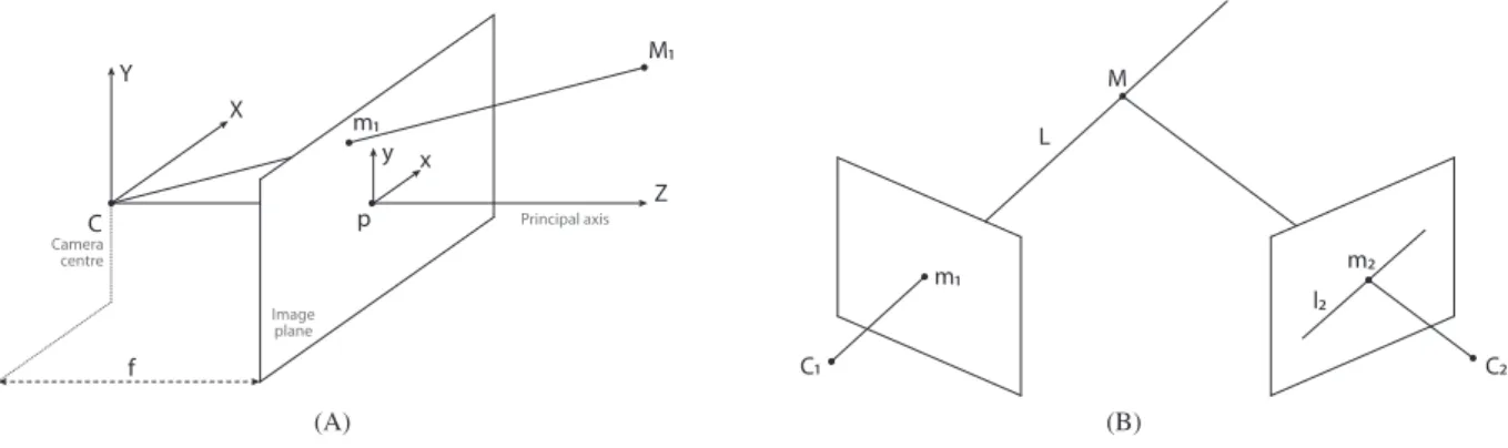
F I G U R E 4 Projective geometry in a pinhole camera. A, Simple scheme showing the projection of a point in the image plane; B, Standard triangulation method where the three-dimensional space coordinates of a point observed from two camera positions can be estimated
from different positions of the same objects are required (and with certain restrictions†) in order to accurately estimate
the 3D position of objects in space using triangulation techniques, also known as Structure from Motion58(Figure 4B).
Figure 4A shows the scheme of a pinhole camera, where C is the camera centre, p is the principal point, f is the focal distance and the image plane represents the plane where the image is formed. M1is any point in the space that is projected
onto m1on the image plane, with coordinates m1 = (m1x, m1y)with respect to the origin p.
The projection of a point from the real 3D space to the image is carried out by the mapping that we have defined as
m = Π(M), and can be written in matrix form as P = K[R|t], where K corresponds to the camera intrinsic matrix and [R|t] represents the camera extrinsic matrix. In its expanded view, the projection can be expressed as
⎡ ⎢ ⎢ ⎢ ⎣ m1x m1y m1s ⎤ ⎥ ⎥ ⎥ ⎦ = ⎡ ⎢ ⎢ ⎢ ⎣ f∕ dx 0 cx 0 0 f∕ dy cy 0 0 0 1 0 ⎤ ⎥ ⎥ ⎥ ⎦ [ R t 0 1 ] ⎡⎢ ⎢ ⎢ ⎢ ⎣ M1x M1y M1z 1 ⎤ ⎥ ⎥ ⎥ ⎥ ⎦ .
The camera extrinsic matrix transforms the original 3D scene points to the camera reference. It can be decomposed in an SO(3) rotation matrix (R) and translation vector (t), and it is used to reference the points observed in the image with respect to a global coordinate system for all frames. The camera intrinsic matrix K applies the projection from 3D camera points into 2D pixel coordinates, and it stores the projection centre (cx, cy), the pixel size (dx, dy) and the focal distance (f ). The third component of m1(m1s) refers to the scaling factor according to the homogeneous coordinate system.
In short, to estimate the position in space of a point M we apply the triangulation process, which is usually done by minimizing the reprojection error d(m, ̂m) on the 2D image, having a set of corresponding points in (at least) two images (although, of course, other techniques exist59). Point ̂m refers to the projected 3D point M in the image.
Since a stereo vision system—see Figure 5—consists of two monocular cameras rigidly joined together, the triangu-lation process can be carried out on each frame (which are actually two images taken at the same time). In addition, the fact that both cameras are rigidly fixed implies that a series of assumptions can be applied to simplify the process, which can be summarized step-by-step below:60
• Image undistortion: lenses used in conventional cameras apply radial and/or tangential distortions that must be
corrected in order to obtain the real image.
• Image rectification: adjustment of the two images captured with the stereo camera to produce alignment and
rectification.
• Correspondences: relate the points observed in the left image with their counterparts in the right image, producing the
disparity map.
• Reprojection: obtaining the depth of each point from the disparity map.
F I G U R E 5 Stereo camera system, where the triangulation process is simplified assuming coplanarity. fleftis the left focal distance, cxleft, cyleftare the points
where the left principal ray is intersecting the left image plane,
Oleftis the origin of the left principal ray, T is the displacement between left and right camera centers and d is the disparity (difference) of the horizontal coordinates of the left and right projections of point P. [Color figure can be viewed at wileyonlinelibrary.com]
As the images from both cameras have been previously undistorted and rectified, the triangulation process is simplified with the known baseline separation between cameras, where the cameras are assumed perfectly coplanar (Figure 5).
Assuming that a point P of the scene is captured by both cameras in pleftand pright, respectively, and that the calibration and rectification processes have been successful, for a frontal parallel camera both points appear on the same vertical coordinate, being ypleft =ypright(row aligned). The difference between the horizontal coordinates defines the disparity d = xpleft−xpright, which can be related to depth by the equation
Z = f T xpleft−xpright
,
where f is the focal length (assuming same value for both cameras) and T is the displacement between camera centers of projection.
Once the geometric problem has been defined, only the points observed in left and right images should be matched to estimate the depth of the scene. This can be done by searching for relevant points extracting features61 or in a
dense way by comparing left and right image by applying energy based techniques.62 The second technique is the
most desirable since it produces a dense map of the scene, estimating depth values for each pixel. As can be expected, this process is computationally expensive, so modern computers equipped with GPUs are used to perform this mas-sive computation. It is usual to obtain frequencies of 30 frames-per-second (fps) for 1080p video resolution or 60 fps for 720 p.‡.
In addition to the online stereo depth perception, a virtual reality system must be self-localized at any time, so it is necessary to merge the depth captured in each frame for all time instants (SLAM). It builds a 3D map of the static objects that surround the camera at the same time the camera trajectory is estimated (Figure 6).
3.4
Collision Estimation
As mentioned before, we employ a pointshell-type algorithm, see Figure 7. Basically, the virtual solid is equipped with a collection of points placed on its boundary. In turn, the physical object is equipped with a level set (distance field), provided by the stereo camera, see Figure 8.
F I G U R E 6 Trajectory of a stereo system, where the path traveled over time is shown by the blue line. The stereo camera estimates the depth in each frame, so it is necessary to merge the information of all frames to create a complete map of the scene. Optionally, it is possible to apply a mesh algorithm to estimate the surface of the objects and get more information about the scene.63[Color figure can be viewed at wileyonlinelibrary.com]
F I G U R E 7 Sketch of the pointshell method for collision detection. The virtual object (in blue) is equipped with a collection of boundary points. Their collision with the zero-distance isosurface of the physical object (in red) is checked at each time step (frame of the video sequence) [Color figure can be viewed at wileyonlinelibrary.com]
In the development of the collision algorithm care must be taken with the limitations imposed by the hardware. In this case, the Zed mini stereo camera is designed to operate in the range of 0.2 to 15 m. Stereo vision algorithms employ triangulations to estimate depth from the disparity of both recorded images. The depth resolution accuracy decreases with distance in a quadratic fashion, with an accuracy of 1% in the near distance to 9% in the far field range.
The particular examples developed herein make intensive use of interactions in the near field range—say, 0.1 to 0.5 m— precisely where the error is minimal. This affects critically the discretization of the contact regions, that will be chosen among the most salient features of the surface of the object. It is simply a waste of computer power to perform a very fine discretization of the contact regions, since the error is limited by the mentioned 1% value given by the camera, much more than usual values for high-fidelity simulations in applied sciences and industry. It is expected, nevertheless, that these values will dramatically decrease in the years to come.
F I G U R E 8 An example of the distance field computed by the stereo camera. Top: original image. Bottom: the computed field as a contour map. It indicates the distance to the camera. Blue objects are closer to the lens, while red objects are farther [Color figure can be viewed at wileyonlinelibrary.com]
At every frame cycle, contact penalty forces are determined by querying the points of the virtual solid Ω2against the
distance field associated to Ω1. This is possible thanks to the fast rates of the stereo camera where the graphic acceleration
ensures real time frequencies to estimate in any frame the depth of each pixel. Therefore, the camera is capable to estimate also the position of dynamic objects, while they are excluded from the SLAM algorithm. It means a natural and robust feeling in the interaction, where static objects are used to locate the camera in space while real dynamic objects are used in the collision estimation.
The computation of 3D distances between virtual and real objects for collision detection is sketched in Algorithm 1.
Algorithm 1. Pseudo-code of the collision-deformation algorithm
matricesMemoryAllocation(3DCoordinatesVirtualObject, 3DCoordinatesStereo); while (True) do
3DCoordinatesStereo = decimate3DStereoData(Raw3DCoordinatesStereo, Nstep);
(dmin, nodeVirtualObject) = parallelizedDistance(3DCoordinatesVirtualObject, 3DCoordinatesStereo);
if (dmin<𝛿Incr) and (deformationPseudoTime < maxDeformationPseudoTime) then
deformationPseudoTime++;
update3DNodePositions(nodeVirtualObject, deformationPseudoTime);
else if (𝛿Incr< dmin<𝛿Decr) and (deformationPseudoTime > minDeformationPseudoTime) then
deformationPseudoTime–;
update3DNodePositions(nodeVirtualObject, deformationPseudoTime); end if
F I G U R E 9 Occlusions implementation to visualize in a natural way the objects that are closer to the camera. Frames extracted from one of our videos (https://www.youtube.com/watch?v=jtMe47mg82k), working in real time and with no postproduction modifications. A, Hand of the user (real object) closer to the camera than the virtual object; B, Virtual object closer to the camera than the hand of the user (real object); C, Interaction between both objects, virtual and real, with the occlusion system working properly [Color figure can be viewed at wileyonlinelibrary.com]
A decimation was applied on the depth image to reduce the computational complexity of estimating distances with the virtual object. Objects of 1 pixel size or less will not appear, in general, inside the normal distance range from the camera, so we consider this simplification has no drawbacks. In addition, there is an intrinsic error associated with estimating depth from disparity map, which means that the tolerance of the 3D reconstruction error may involve noise in the estimation of the correct depth for 1 pixel objects. The decimation is only applied to the distance estimation algorithm, so that the visualization process is carried out in high resolution.
As can be seen in Algorithm 1, contact with the virtual object is only allowed at one point of the contour per instant, since deformation does not comply with the principle of superposition when the material does not follow a linear behavior. In the case that more than one contact point at a time is desired, new simulations need to be precomputed including these new loading states. Thus, the manifold obtained after applying the MOR method to project the solution would store all that new information.
3.5
Visualization
To visualize all the content in a smooth way we used OpenGL, that allows to render primitives in an efficient way get-ting real-time rates (the maximum frequency of visualization is imposed by the capture frequency of the stereo camera). Thanks to the simplicity and optimization of OpenGL we added lighting effects that translate into a more natural visu-alization of virtual objects, fitting better into the real scene. It is not our goal to create a hyper-realistic rendering, so we have employed basic visualization techniques.
Occlusions are a characteristic that gives a natural behavior to the augmented reality interaction. However, its com-putation is one of the most complex tasks, since it is not easy to perfectly estimate the depth of all objects to draw in front those that are closest to the camera. This procedure is known as Z-culling, a term used in the computer graphics commu-nity for this process.64Since the stereo camera estimates the depth of all the pixels in the image, we have implemented a
small algorithm capable of applying occlusions to the video sequence in real time. For this task we use shaders (written in OpenGL Shading Language or GLSL, see https://www.khronos.org/opengl/wiki/Core_Language_(GLSL)), which are small programs that run directly on the GPU and are able to perform simple tasks in parallel and very efficiently. Occlu-sions are estimated between real and virtual objects for each pixel of the image as a function of the distance to the camera, see Fig. 9. It is important to notice that we are not using object recognition techniques, but only the depth information from the stereo camera.
4
DATA A S S I M I L AT I O N P RO C E S S
The fusion of all ingredients described in previous sections builds the whole method. It is the interaction between all of them where the advantage lies, and we understand this process as a particular instance of data assimilation: collecting
F I G U R E 10 Beams location in space. Load is applied in the upper face of the blue beam and when it deforms enough, contact between both beams arises [Color figure can be viewed at wileyonlinelibrary.com]
data that comes from the images so as to determine the particular values of parameters in our physical model and to finally visualize the updated result of these models.
Data come directly from the camera where, thanks to the contact algorithm, the contact (loading) point xcontactand the
displacement u(xcontact)are estimated. Displacements are related to the module of the applied load, so with it is
straight-forward to reconstruct the particular solution for that set of parameters𝝁contact= (xcontact, u(xcontact)). This reconstruction
is actually a mapping from the reduced, low-dimensional space to the original space where the high-fidelity solution lies. The displacements and the stress field can then be plotted on the object at video frequency (30 frames per second).
4.1
Implementation details
We used a stereo camera from StereoLabs, model ZED Mini. To carry out all computational tasks we use a workstation with an Intel Core i7-8700K CPU, where the graphics part was the most critical since the stereo camera needs graphic acceleration, for which we used a Nvidia GeForce RTX 2070. We used and integrated the SDK of the stereo camera with our own code, where the functions to obtain the depth of the camera and the SLAM fusion have been provided by the manufacturer.
5
E X P E R I M E N TA L R E S U LT S
In this section we show three different examples to show the potentialities of our method. The first example shows the con-tact between two virtual objects and any real object. Subsequent examples consider only one virtual object, but interaction is allowed with any object of the physical environment.
5.1
Cantilever beams
The first example consists of two cantilever beams placed perpendicularly, where free ends of both beams overlap, being that part where contact occurs (see Figure 10).
Both beams are made of a hyperelastic material (Saint Venant-Kirchhoff), where the energy density function can be expressed as
Ψ(E) = 1
2𝜆[tr(E)]
2
+𝜇E ∶ E.
We applied the PGD method in its classical, intrusive standard version with one parameter s that serves to parameter-ize the position of load t. For more details of this implementation, the reader is referred to previous works of the authors, see, for instance, Reference 65. The code for this problem is available at Reference 66. The solution in separate variables
takes the form
u(X, s) ≈
n∑mod i=1
Fi(X)Gi(s), (4)
where X = (X, Y, Z) are the reference coordinates of each beam node, s = (sX, sY)are the application positions of the load on the top face of the blue beam (see Figure 10) and nmodis the number of modes needed to approximate the solution. To
obtain the solution evaluated for a specific position of the load in the original high-dimensional space it is necessary to particularize the solution at a value of s, which is computed by simple multiplications.
The weak form of the equation to solve, therefore, is expressed as
∫Γ∫Ω
𝜵su∗∶𝝈 dΩdΓ = ∫
Γ∫Γ
u∗ t dΓdΓ, (5)
where Ω represents the volumetric solid, Γ is the boundary region discretized by s where the load can be applied, u∗is
the test function,𝛁sthe symmetric gradient operator, “∶” the double contraction operator,𝝈 the stress tensor and t the
load applied at the boundary. The load function can be separated as
t ≈
M
∑
j=1
fj(X)gj(s). (6)
By substituting Equations (4) and (6) into (5), it is possible to solve the parametric problem by projecting the solution into separate spaces (intrusively). For more information about the PGD application to the nonlinear equation of Saint Venant-Kirchhoff, reader can consult,67and for more information about the original PGD method (intrusive) applied to
differential equations, see.44
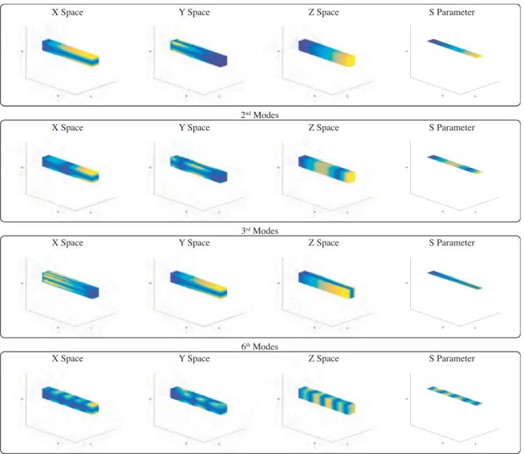
The mesh used has a total of 3381 nodes with 6758 elements in space, while the number of nodes for the s parameter are 1749 (possible load positions). More information about the implementation can be found in Reference 12. The result of some of the spatial modes as well as those for the s parameter can be seen in Figure 11. In the case of modes related to the parameter s, we plot only the upper surface, since the load can only be applied within that domain.
The parametric solution obtained for the contact in one beam is actually applied on both beams, since the problem to be solved is the same, although the origin of the load is different. For the upper beam, contact is made with any real object captured by the stereo camera. For the lower beam, contact is produced by the deformed upper beam (which in turn has been deformed with the contact of the real object) and therefore the load is assumed to be always vertical. Therefore, we have solved the problem only once, although the solution is evaluated online in two beams.
The resulting sequence can be seen at https://youtu.be/PaK7STfWGfs. Some frames are shown in Figure 12.
5.2
Stanford Bunny
The second example uses the Stanford bunny68as virtual object to deform. The material law applied is homogeneous and
isotropic throughout the solid, with a Neo-Hookean compressible hyperelastic model. The energy density function can be expressed as
Ψ =C1(I1−3 − 2lnJ) + D1(lnJ)2, (7)
being C1and D1material constants, J = det(F), with F the deformation gradient and I1the first deviatoric strain invariant
defined as
I1=𝜆21+𝜆22+𝜆23, (8)
where𝜆i=J−1∕3𝜆i. In this problem, we used the Non-Intrusive PGD method by making external calls to the well-known
F I G U R E 11 Modes of the cantilever beam example. The three first columns represent the three first components, respectively, of the modes Fi(X), for i = 1, 2, 3, and 6. The fourth column represents the modes Gi(s)[Color figure can be viewed at wileyonlinelibrary.com]
information, and modes Gidepend on s, that defines the position and module of the load. To simplify the problem, all
loads are applied in the direction of the center of mass of the object. The discretization of the geometry is composed by a mesh of 16 519 nodes and 87 916 elements, where we defined 34 possible contact points where the force is gradually applied during 26 pseudo-time increments. However, to reduce the cost of visualization we only show boundary nodes (although calculations have been made with all the nodes), being reduced to 3733 nodes and 7462 elements. The result of the modes in space and stress can be seen in Figure 13.
Each sampling point s of the Stanford bunny problem takes in Abaqus more than 34 minutes running on a PC equipped with Intel i5 chipset at 2.9 GHz. As can readily be noticed, direct computation is far from being a solution for real-time frequencies. And most likely will continue to be so in the near future.
Figure 14 plots the L2-norm error made by the approximation in the projection.
Finally, Figure 15 shows four frames extracted from a video sequence (https://www.youtube.com/watch?v= lmApbJA6gH4) recorded in a desktop. They show a person interacting with the virtual object touching it in different points, using his own hands but any other object could be used.
F I G U R E 12 Two frames of the contacting beams sequence [Color figure can be viewed at wileyonlinelibrary.com]
F I G U R E 13 Spatial modes for the Stanford bunny problem [Color figure can be viewed at wileyonlinelibrary.com]
5.3
Stanford Dragon
The third and last example uses the Stanford dragon68as a deformable virtual object. The material law is the same as
for the Stanford bunny. The number of possible contact points in this case is 32 (Figure 16, right) with 16 pseudo-time increments to apply the loads progressively. Since the geometry of the dragon is more intricate than the bunny one, the directions of application of the loads follow the normal directions to the planes that form each set of load application points. The dragon mesh is discretized in 22 982 nodes and 46 540 elements. Up to 200 modes have been considered in our PGD reduced-order model, see Figure 17.
As in the bunny example, we plot the error reconstruction due to projection in Figure 18. Figure 19 shows four frames extracted from the same video sequence than the bunny. Here the user is touching two points of the dragon contour producing displacements and showing in color the stress map that the contact generates.
F I G U R E 14 L2-norm error due to the projection process for the Stanford bunny [Color figure can be viewed at
wileyonlinelibrary.com]
F I G U R E 15 Some frames extracted from the bunny sequence. Colors show the stress map associated with the deformations imposed by contact with real objects [Color figure can be viewed at wileyonlinelibrary.com]
F I G U R E 16 Contact points for the Stanford bunny and dragon. The applied loads simulating contact are centered on the orange dots and have an application range of two neighbors (graph distance), marked in the figure with yellow and violet colors) [Color figure can be viewed at wileyonlinelibrary.com]
F I G U R E 17 Spatial modes for the Stanford dragon problem [Color figure can be viewed at wileyonlinelibrary.com]
F I G U R E 18 Reconstruction errors due to the projection process for the Stanford dragon. The left graph shows the L2-norm error, the center one shows the median error along the different load positions, and the right one shows the maximum error for any loading point and any pseudo-time increment [Color figure can be viewed at wileyonlinelibrary.com]
F I G U R E 19 Some frames extracted from the dragon sequence. Colors show the stress map associated with the deformations imposed by contact with real objects [Color figure can be viewed at wileyonlinelibrary.com]
6
CO N C LU S I O N S
In this work we present a method for the real-time interaction of virtual and physical objects in MR applications. Three examples are analyzed that showed real-time performance in our experiments. Although the examples may seem related to the entertainment industry we would like to note the relevance that this type of work could have in other areas such as surgery or industry. The visualization of relevant data in real time has an enormous importance in decision-making, and by relevant data we mean visual information that our eyes cannot perceive directly. In the mechanical case we are talking about stress distribution in a solid, but we could talk about any other physical phenomenon that provides information with physical sense and a simple and natural user interaction.
We believe that the introduction of MOR methods has much to say in this field. We have used several methods, but of course there are many other MOR methods, each with its own advantages, which can be applied in the visualization of data in real time. Physical engines (such as those used in video games) serve to greatly simplify physical equations working at video frequencies, but the results are far from what we really want to solve: high-fidelity models.
Visualization tasks and measurements with the camera are possible here thanks to the graphic acceleration. In our case we used a workstation, but nowadays it is also possible to use mobile devices with graphical acceleration, although of course the resolution is drastically reduced to maintain video frequencies around 30 fps. The problem of occlusions has been treated in this work by brute force, analyzing the depth of each pixel by graphical acceleration and GLSL shaders, but it is still an open problem, where some works use dense segmentations of objects in images, see https://developer. apple.com/augmented-reality/arkit/. Using a stereo camera, some small errors may appear in the measurement of the depth, which are usually due to areas not visible from both cameras at the same time, or surfaces that are oriented in the direction of the camera projecting rays. However, there are some works to correct these effects in geometry and texture by applying neural networks.69Sometimes, spurious effects are perceived due to the difficult identification of depth in a
flat image, when the video stream is being observed from the computer screen, for instance. Implementations on stereo glasses such as Hololens or similar are expected to very much improve this sensation of realism.
AC K N OW L E D G E M E N T S
This project has been partially funded by the ESI Group through the ESI Chair at ENSAM ParisTech and through the project “Simulated Reality” at the University of Zaragoza. The support of the Spanish Ministry of Economy and Com-petitiveness through grant number CICYT-DPI2017-85139-C2-1-R and by the Regional Government of Aragon and the European Social Fund, are also gratefully acknowledged.
CO N F L I CT O F I N T E R E ST S
The authors declare that they have no conflict of interest.
O RC I D
Elías Cueto https://orcid.org/0000-0003-1017-4381
R E F E R E N C E S
1. Mur-Artal R, Montiel JMM, Tardos JD. ORB-SLAM: a versatile and accurate monocular SLAM system. IEEE Trans Robot. 2015;31(5):1147-1163.
2. Engel J, Schöps T, Cremers D. LSD-SLAM: large-scale direct monocular SLAM. European Conf Comput Vision. 2014;834-849.
3. Fedorov R, Frajberg D, Fraternali P. A framework for outdoor mobile augmented reality and its application to mountain peak detec-tion. Paper presented at: Proceedings of the International Conference on Augmented Reality, Virtual Reality and Computer Graphics; 2016:281-301.
4. Paavilainen J, Korhonen H, Alha K, Stenros J, Koskinen E, Mayra F. The Pokémon GO experience: a location-based augmented reality mobile game goes mainstream. Paper presented at: Proceedings of the 2017 CHI Conference on Human Factors in Computing Systems; 2017:2493-2498.
5. Haouchine N, Dequidt J, Kerrien E, Berger MO, Cotin S. Physics-based augmented reality for 3D deformable object. Paper presented at: Proceedings of the Eurographics Workshop on Virtual Reality Interaction and Physical Simulation; 2012; Darmstadt, Germany.
6. Wriggers P, Zavarise G. Computational contact mechanics. Encyclopedia of Computational Mechanics. Chichester: Wiley; 2004.
7. Teschner M, Kimmerle S, Heidelberger B, et al. Collision detection for deformable objects. Comput Graph Forum. 2005;24(1):61-81. https:// doi.org/10.1111/j.1467-8659.2005.00829.x.
8. Chaudhary AB, Bathe KJ. A solution method for static and dynamic analysis of three-dimensional contact problems with friction. Comput
9. Períc D, Owen D. Computational model for 3-D contact problems with friction based on the penalty method. Int J Numer Methods Eng. 1992;35(6):1289-1309.
10. Simo J, Laursen T. An augmented Lagrangian treatment of contact problems involving friction. Comput Struct. 1992;42(1):97-116. 11. Brunßen S, Hüeber S, Wohlmuth B. Contact dynamics with Lagrange multipliers. IUTAM Symp Comput Methods Contact Mech.
2007;17-32.
12. González D, Alfaro I, Quesada C, Cueto E, Chinesta F. Computational vademecums for the real-time simulation of haptic collision between nonlinear solids. Comput Methods Appl Mech Eng. 2015;283:210-223.
13. Breen DE, Rose E, Whitaker RT. Interactive Occlusion and Collision of Real and Virtual Objects in Augmented Reality. Munich, Germany: European Computer Industry Research Center; 1995.
14. Takeuchi I, Koike T. Augmented reality system with collision response simulation using measured coefficient of restitution of real objects. Paper presented at: Proceedings of the 23rd ACM Symposium on Virtual Reality Software and Technology; 2017:49; ACM.
15. Montero A, Zarraonandia T, Diaz P, Aedo I. Designing and implementing interactive and realistic augmented reality experiences. Univ
Access Inf Soc. 2019;18(1):49-61.
16. Fulton L, Modi V, Duvenaud D, Levin DIW, Jacobson A. Latent-space dynamics for reduced deformable simulation. Comput Graph Forum. 2019;38(2):379-391.
17. Berkooz G, Holmes P, Lumley JL. The proper orthogonal decomposition in the analysis of turbulent flows. Ann Rev Fluid Mech. 1993;25(1):539-575.
18. Chaturantabut S, Sorensen DC. Nonlinear model reduction via discrete empirical interpolation. SIAM J Sci Comput. 2010;32(5):2737-2764. 19. Amsallem D, Zahr MJ, Farhat C. Nonlinear model order reduction based on local reduce order bases. Int J Numer Methods Eng.
2012;92(10):891-916.
20. Badias A, González D, Alfaro I, Chinesta F, Cueto E. Local proper generalized decomposition. Int J Numer Methods Eng. 2017;112(12):1715-1732.
21. Smola A, Müller KR. Kernel principal component analysis. In: Gerstner W, Germond A, Hasler M, Nicoud JD. (eds) Artificial Neural Networks—ICANN’97. ICANN 1997. Lecture Notes in Computer Science, vol 1327. Berlin, Heidelberg: Springer; 1997.
22. Roweis ST, Saul LK. Nonlinear dimensionality reduction by locally linear embedding. Science. 2000;290(5500):2323-2326.
23. Krenciszek J, Pinnau R. Model reduction of contact problems in elasticity: proper orthogonal decomposition for variational inequalities.
Progress in Industrial Mathematics at ECMI 2012. New York, NY: Springer; 2014:277-284.
24. Petrov E. A high-accuracy model reduction for analysis of nonlinear vibrations in structures with contact interfaces. J Eng Gas Turb Power. 2011;133(10):102503.
25. Xie S, Girshick R, Dollár P, Tu Z, He K. Aggregated residual transformations for deep neural networks. Paper presented at: Proceedings of the IEEE Conference on Computer Vision and Pattern Recognition; 2017:1492-1500.
26. Redmon J, Farhadi A. Yolov3: An incremental improvement; 2018. arXiv preprint arXiv:1804.02767.
27. Young T, Hazarika D, Poria S, Cambria E. Recent trends in deep learning based natural language processing. IEEE Comput Intell Mag. 2018;13(3):55-75.
28. Payne C. OpenAI MuseNet. openai.com/blog/musenet.
29. Bailey SW, Otte D, Dilorenzo P, O'Brien JF. Fast and deep deformation approximations. ACM Trans Graph (TOG). 2018;37(4):119. 30. Raissi M, Perdikaris P, Karniadakis GE. Physics informed deep learning (part i): Data-driven solutions of nonlinear partial differential
equations; 2017. arXiv preprint arXiv:1711.10561.
31. Lee K, Carlberg K. Model reduction of dynamical systems on nonlinear manifolds using deep convolutional autoencoders; 2018. arXiv preprint arXiv:1812.08373.
32. Kölsch M, Turk M. Robust hand detection. Proceedings of the FGR'04; 2004:614-619.
33. Suarez J, Murphy RR. Hand gesture recognition with depth images: a review. Paper presented at: Proceedings of the 21st IEEE International Symposium on Robot and Human Interactive Communication 2012 IEEE RO-MAN; 2012:411-417.
34. Potter LE, Araullo J, Carter L. The leap motion controller: a view on sign language. Paper presented at: Proceedings of the 25th Australian Computer-Human Interaction Conference: Augmentation, Application, Innovation, Collaboration; 2013:75-178.
35. Ren Z, Yuan J, Meng J, Zhang Z. Robust part-based hand gesture recognition using Kinect sensor. IEEE Trans Multimedia. 2013;15(5):1110-1120.
36. Chaconas N, Höllerer T. An evaluation of bimanual gestures on the microsoft hololens. Paper presented at: Proceedings of the 2018 IEEE Conference on Virtual Reality and 3D User Interfaces (VR); 2018:1-8.
37. Quesada C, Alfaro I, González D, Chinesta F, Cueto E. Haptic simulation of tissue tearing during surgery. Int J Numerical Methods Biomed
Eng. 2018;34(3):e2926.
38. Perret J, Vander Poorten E. Touching virtual reality: a review of haptic gloves. Paper presented at: Proceedings of the 16th International Conference on New Actuators (ACTUATOR 2018); 2018:1-5.
39. Lundgren B. A demonstration of vertical planes tracking and occlusions with ARKit+Scenekit. https://github.com/bjarnel/arkit-occlusion.
40. Barbiˇc J, James DL. Six-DoF haptic rendering of contact between geometrically complex reduced deformable models. IEEE Transactions
on Haptics. 2008;1(1):39-52. https://doi.org/10.1109/TOH.2008.1.
41. Badias A, Curtit S, Gonzalez D, Alfaro I, Chinesta F, Cueto E. An augmented reality platform for interactive aerodynamic design and analysis. Int J Numer Methods Eng. 2019;120(1):125-138. https://doi.org/10.1002/nme.6127.
42. Chinesta F, Aguado JV, Abisset-Chavanne E, Barasinski A. Model reduction & manifold learning—based parametric computational electromagnetism: fundamentals & applications. Paper presented at: Proceedings of the2016 IEEE Conference on Electromagnetic Field Computation (CEFC); 2016:1.
43. Reddy JN. An Introduction to Continuum Mechanics. Cambridge, MA: Cambridge University Press; 2013.
44. Ammar A, Mokdad B, Chinesta F, Keunings R. A new family of solvers for some classes of multidimensional partial differential equations encountered in kinetic theory modeling of complex fluids. J Non-Newtonian Fluid Mech. 2006;139(3):153-176.
45. Chinesta F, Keunings R, Leygue A. The Proper Generalized Decomposition for Advanced Numerical Simulations: A Primer. Springer Science & Business Media; 2013.
46. Ibáñez R, Abisset-Chavanne E, Ammar A, et al. A multidimensional data-driven sparse identification technique: the sparse proper generalized decomposition. Complexity. 2018;2018:5608286.
47. Zou X, Conti M, Diez P, Auricchio F. A nonintrusive proper generalized decomposition scheme with application in biomechanics. Int
J Numer Methods Eng. 2018;113(2):230-251.
48. Chinesta F, Cueto E. PGD-Based Modeling of Materials, Structures and Processes. Switzerland: Springer International Publishing; 2014. 49. Aguado J, Borzacchiello D, Kollepara KS, Chinesta F, Huerta A. Tensor representation of non-linear models using cross approximations.
J Sci Comput. 2019;1-26. https://doi.org/10.1007/s10915-019-00917-2
50. Niroomandi S, Alfaro I, Cueto E, Chinesta F. Model order reduction for hyperelastic materials. Int J Numer Methods Eng. 2010;81(9):1180-1206.
51. De Lathauwer L, De Moor B, Vandewalle J. A multilinear singular value decomposition. SIAM J Matrix Anal Appl. 2000;21(4):1253-1278. 52. Andersson CA, Bro R. Improving the speed of multi-way algorithms: Part I. tucker3. Chemometr Intell Laborat Syst. 1998;42(1-2):93-103. 53. Tucker LR. Some mathematical notes on three-mode factor analysis. Psychometrika. 1966;31(3):279-311.
54. Bro R. PARAFAC Tutorial and applications. Chemometr Intell Laborat Syst. 1997;38(2):149-171.
55. Hartley R, Zisserman A. Multiple View Geometry in Computer Vision. Cambridge, MA: Cambridge University Press; 2003.
56. Liu F, Shen C, Lin G. Deep convolutional neural fields for depth estimation from a single image. Paper presented at: Proceedings of the IEEE Conference on Computer Vision and Pattern Recognition; 2015:5162-5170.
57. Facil JM, Ummenhofer B, Zhou H, Montesano L, Brox T, Civera J. CAM-Convs: camera-aware multi-scale convolutions for single-view depth. Paper presented at: Proceedings of the IEEE Conference on Computer Vision and Pattern Recognition; 2019:11826-11835. 58. Ullman S. The interpretation of structure from motion. Proc Royal Soc London Ser B Biol Sci. 1979;203(1153):405-426.
59. Lee SH, Civera J. Triangulation: why Optimize? 2019. arXiv e-prints 2019: arXiv:1907.11917.
60. Bradski G, Kaehler A. Learning OpenCV: Computer Vision with the OpenCV Library. O'Reilly Media, Inc; 2008.
61. Fua P. A parallel stereo algorithm that produces dense depth maps and preserves image features. Mach Vis Appl. 1993;6(1):35-49. 62. Alvarez L, Deriche R, Sanchez J, Weickert J. Dense disparity map estimation respecting image discontinuities: a PDE and scale-space
based approach. J Visual Commun Image Represent. 2002;13(1-2):3-21.
63. Lin HW, Tai CL, Wang GJ. A mesh reconstruction algorithm driven by an intrinsic property of a point cloud. Comput-Aid Des. 2004;36(1):1-9.
64. Greene N, Kass M, Miller G. Hierarchical Z-buffer visibility. Proceedings of the 20th Annual Conference on Computer Graphics and Interactive Techniques; 1993:231-238.
65. Niroomandi S, Gonzalez D, Alfaro I, Cueto E, Chinesta F. Model order reduction in hyperelasticity: a proper generalized decomposition approach. Int J Numer Methods Eng. 2013;96(3):129-149. https://doi.org/10.1002/nme.4531.
66. Cueto E, González D, Alfaro I. Proper Generalized Decompositions: An Introduction to Computer Implementation with Matlab. New York, NY: Springer Briefs in Applied Sciences and Technology Springer International Publishing; 2016.
67. Niroomandi S, Gonzalez D, Alfaro I, et al. Real-time simulation of biological soft tissues: a PGD approach. Int J Numer Methods Biomed
Eng. 2013;29(5):586-600.
68. The stanford 3D scanning repository. http://graphics.stanford.edu/data/3Dscanrep/.
69. Martin-Brualla R, Pandey R, Yang S, et al. LookinGood: enhancing performance capture with real-time neural re-rendering. SIGGRAPH Asia 2018 Technical Papers; 2018:255.