Science Arts & Métiers (SAM)
is an open access repository that collects the work of Arts et Métiers Institute of
Technology researchers and makes it freely available over the web where possible.
This is an author-deposited version published in: https://sam.ensam.eu Handle ID: .http://hdl.handle.net/10985/12915
To cite this version :
Pascal POMAREDE, Fodil MERAGHNI, Laurent PELTIER, Stéphane DELALANDE, Nico Felicien DECLERCQ - Damage Evaluation in Woven Glass Reinforced Polyamide 6.6/6 Composites Using Ultrasound Phase-Shift Analysis and X-ray Tomography - Journal of Nondestructive Evaluation - Vol. 37, p.12 - 2018
Any correspondence concerning this service should be sent to the repository Administrator : archiveouverte@ensam.eu
Science Arts & Métiers (SAM)
is an open access repository that collects the work of Arts et Métiers ParisTech
researchers and makes it freely available over the web where possible.
This is an author-deposited version published in: http://sam.ensam.eu Handle ID: .http://hdl.handle.net/null
To cite this version :
Pascal POMAREDE, Fodil MERAGHNI, Laurent PELTIER, Stephane DELALANDE, Nico F. DECLERCQ - Damage Evaluation in Woven Glass Reinforced Polyamide 6.6/6 Composites Using Ultrasound Phase-Shift Analysis and X-ray Tomography - Journal of Nondestructive Evaluation - Vol. 37, p.12 - 2018
Any correspondence concerning this service should be sent to the repository Administrator : archiveouverte@ensam.eu
Damage Evaluation in Woven Glass Reinforced Polyamide 6.6/6
Composites Using Ultrasound Phase-Shift Analysis and X-ray
Tomography
Pascal Pomarède1,2 · Fodil Meraghni1 · Laurent Peltier1 · Stéphane Delalande3 · Nico F. Declercq2,4
Abstract
The paper proposes a new experimental methodology, based on ultrasonic measurements, that aims at evaluating the anisotropic damage in woven semi-crystalline polymer composites through new damage indicators. Due to their microstructure, woven composite materials are characterized by an anisotropic evolution of damage induced by different damage mechanisms occurring at the micro or mesoscopic scales. In this work, these damage modes in polyamide 6.6/6-woven glass fiber reinforced composites have been investigated qualitatively and quantitatively by X-ray micro-computed tomography (mCT) analysis on composite samples cut according to two orientations with respect to the mold flow direction. Composite samples are initially damaged at different levels during preliminary interrupted tensile tests. Ultrasonic investigations using C-scan imaging have been carried out without yielding significant results. Consequently, an ultrasonic method for stiffness constants estimation based on the bulk and guided wave velocity measurements is applied. Two damage indicators are then proposed. The first consists in calculating the Frobenius norm of the obtained stiffness matrix. The second is computed using the phase shift between two ultrasonic signals respectively measured on the tested samples and an undamaged reference sample. Both X-ray mCT and ultrasonic investigations show a higher damage evolution with respect to the applied stress for the samples oriented at 45◦ from the warp direction compared to the samples in the 0◦ configuration. The evolution of the second ultrasonic damage indicator exhibits a good correlation with the void volume fraction evolution estimated by mCT as well as with the damage calculated using the measured elastic modulus reduction. The merit of this research is of importance for the automotive industry.
Keywords Composite materials · Ultrasonics · X-ray tomography · Damage Indicator
1 Introduction
Woven reinforced thermoplastic composite materials are gaining interest in automotive applications [1–3], due to their important weight reduction in comparison with applications using metals. In addition, compared to a unidirectional
rein-forcement, a woven fabric allows a better equilibrium and uniformity of the mechanical properties. Furthermore, they also have a better ability to withstand buckling and impact [4]. The latter characteristic is of critical interest for the automotive industry [5]; indeed it is essential to ensure a maximal resistance of structural parts, in the case of impact in particular for the driver’s safety. To assess the in-service strength of an automotive component made of woven fab- ric composite that is subjected to damage accumulation, the development of an efficient methodology evaluating the dam- age is mandatory. This assessment should guide decisions to replace, to repair or to keep a composite component based on its damage tolerance. Non-destructive methods based on ultrasonic investigation naturally emerge as promising damage evaluation techniques thanks to their practicality, efficiency, diversity and their applicability on composite parts in-service. Nevertheless, ultrasonic techniques require
appropriate signal processing to extract damage indicators that permit estimation of the residual stiffness, which is related to the component integrity.
In order to nondestructively assess all the elastic constants
of a material, Markham [6] has studied a method based on
ultrasonic measurements in immersion of bulk wave veloci- ties and the use of the well-known Christoffel equation. He applied the method on an undamaged transversely isotropic composite material to determine the stiffness components. The method was then successfully used to measure the stiff- ness reduction of composites submitted to different levels of impact [7,8] and tensile tests [9,10]. One of the advan- tages of this method is that the tested material is investigated in all directions (i.e. sample orientations) and therefore can provide all the components of the stiffness tensor and accord- ingly a complete anisotropic damage evaluation of the tested sample. This method was also extended for use with guided waves in several studies because of their established advan- tages [11,12]. In the industry one normally do not require full understanding of all physical phenomena involved but rather seek practical and workable techniques that are reli- able. To our knowledge, no damage indicator, with simple interpretation, useful in the industry, for the global damage state, has been reported in the literature. Such task is carried out here, where an experimental methodology is developed for identifying proper damage indicators.
An alternative method, somewhat similar to the method proposed by Markham, is the polar-scan method [13,14]. As indicated by its name, a specific point of a sample is scanned for all accessible angles of incidence. For each polar angle, the signal amplitude is recorded and represented in a polar plot. Information such as damage level, stiffness, fiber misalignment, etc can be extracted from this polar figure. However, this technique requires a more complex appa- ratus than the one proposed by Markham because of the unavoidable double angular rotations. This limits therefore its application on site (in-service). Due to this limitation, the present approach measures the elastic constants using the ultrasonic method based on wave velocities measurement and described in the preceding paragraph. The aim of this study is then to propose an ultrasonic methodology to detect and to quantify damage growth, even when the cracks that propagate inside the sample cannot be detected by classical ultrasonic imaging techniques. As mentioned, this method could provide the whole stiffness tensor of a sample. How- ever, it is more interesting to obtain a sole value to efficiently transcribe the global damage state of a tested sample. Two different experimental damage indicators are proposed for this purpose: The first is the norm of the stiffness tensor and the second is the phase angle shift between wave signals propagated through a damaged and an undamaged sample. It is worth noting that the time required to analyze the
exper-imental results in order to obtain the first indicator can be quite long.
The woven reinforced composite material exhibits a spe- cific damage scheme that is highly dependent on both the loading direction and the fiber orientation [15,16]. In this work, the damage characterization and evolution was performed on samples made of co-polyamide 6.6/6 based composites reinforced with woven glass fibers and submit- ted to tension tests interrupted at different stress levels. Two configurations of material samples were tested: (i) samples oriented at 0◦ with respect to the warp direction and (ii) sam-ples oriented at 45◦ from the warp direction corresponding to the mold flow direction. A first damage estimation for the two samples configurations was carried out using the elastic modulus reduction. Various nondestructive tests were performed on the samples after loading, such as ultrasonic C- scan imaging that was not able to capture the damage zone in all tested samples. To address this aspect, the damage mecha- nisms induced by the different tensile tests were investigated by X-ray micro-computed tomography (mCT). This provided a qualitative description of the main damage mechanisms and the quantitative estimation of void volume fraction evolution. The latter was compared to the damage indicators evolution obtained with the ultrasonic technique.
The paper is organized as follows: in Sect. 2 the inves- tigated composite material and the tensile tests procedure are presented. Ultrasonic C-scan imaging results obtained on samples after interrupted tensile tests are presented and discussed. X-ray mCT investigation procedure and results, on samples in both 0◦ and 45◦ configurations are discussed in Sect. 3. Ultrasonic analysis and the estimation of the dam- age evolution are presented in the 4th section. The evolution of the stiffness components function of the applied stress level is also discussed for both 0◦ and 45◦ samples. In Sect.
5, the two proposed damage indicators are calculated using
the ultrasonic results from the previous section. Both ultra- sonic damaged indicators are compared with the estimation of damage calculated using the elastic modulus reduction (presented in Sect. 2) and with the void volume fraction evo- lution (discussed in Sect. 3) leading to concluding remarks.
2 Material Description and Preliminary Tests
2.1 Material
The composite material considered for this study is refer- enced as VizilonTM SB63G1-T1.5-S3 and is manufactured by DuPont. The studied composite is produced by a thermo- compression molding process and it consists of a 2/2 twill weave glass fabric reinforced co-polyamide 6.6/6, with three plies, of 1.53 mm thick in total. The overall 3D woven fabric of the studied composite material is shown in Fig. 1. The
E
2. The two different microstructures can be observed in the
Fig. 3. All the samples are stored in a humidity chamber in order to have the same initial conditions in terms of relative humidity. The latter is set at a level of 50% for all tested composite material. Initial tensile tests are performed on the material until failure for both 0◦ and 45◦ sample configura-tions. The experimental stress/strain curves are normalized with respect of the tensile ultimate strength of the 0◦ sample configuration.
Fig. 1 Overall 3D mesostructure of the studied composite consisting
of 2/2 twill weave fabric reinforced polyamide 6.6/6 matrix
Fig. 2 Position of the samples oriented at 0◦ and 45◦ with respect to the warp direction assumed as the mold flow direction of the composite plate
2.2 Tensile Tests Procedure
The tested samples are subjected to an interrupted tensile loading at different levels. For 45◦ samples configuration, the tensile tests are interrupted at the following stress levels: 0, 30.5, 61.1, and 91.6% of σ UTS45◦ , whereas for 0◦ config-uration, the interruption occurs at the levels of 0, 30.8, 46.3, 61.7, 77.2, and 92.6% of σ UTS0◦ . The chosen loading values
are schematically illustrated by means of red circles on the representative stress/strain curves in Fig. 4. All the tensile tests presented in this paper follow the same procedure.
To estimate the modulus reduction caused by these inter- rupted tensile tests, the samples are loaded to the prefixed stress values and then are unloaded (elastic release) back to zero force. The evolution of damage was computed as:
En
weight fiber content is 63% corresponding to a fiber volume
D = 1 −
0
(1)
fraction of 43%. Ten samples are cut in rectangular plate of 45 mm length and 150 mm width. Four samples are cut at 45◦ with respect to the warp direction (mold flow direction) and six other ones are cut along the warp direction. The ori- entations of these two sets of samples are indicated in Fig.
Where E0 is the elastic modulus of the tested sample during
the first loading and En represents the Young’s modulus of the
tested sample during the elastic release. The E0 is estimated
for every single sample between 0.2% and 0.4% of strain
according to the standard ISO 527. The En values are
cal-Fig. 3 Cross-sectional
observation with optical microscope of the 2/2 twill weave fabric reinforced polyamide composite microstructure for samples oriented at 0◦ and 45◦. a 0◦ sample, b 45◦ sample and c Zoom-in on a sample’s yarns in the 0◦ orientation
Longitudinal yarn
(a)
Resin rich area
Tension loading direction
Transversal yarn
500 um
(b) (c)
17 um
+45° -45° Resin rich area
Fig. 4 Typical stress/strain responses of the 2/2 twill weave fabric rein-
forced polyamide composite under tension at 0◦ and 45◦. The red circles show schematicaly where the tensile tests have been interupted for both tested configurations
culated after the unloading according to a common damage measurement procedure [17]. A representation of the elastic moduli calculation is depicted in Fig. 5a, b for the two tested sample configurations.
The samples are all loaded in tension at room temperature and at a constant strain rate of 10−4 s−1 to avoid the influ-ence of viscosity. Tensile tests are performed in compliance with the standard ISO 5893 on a machine Z 050 designed by Zwick Roell. The strains are measured using a “clip-on” extensometer manufactured by Epsilon Technology Corp.
As shown in Fig. 5, a noticeable difference is observed between the overall stress-strain responses of the two config-uration samples, namely 0◦ and 45◦. In fact, for the samples tested at 0◦, the behavior in tension is mostly linear and brittle since it is governed by the fiber breakage whereas the
behav-ior of the samples tested at 45◦ exhibits a nonlinear ductile response mostly governed by the matrix rheology.
This is particularly clear for the evolution of the damage estimated on the elastic modulus reduction when the applied stress increases, as illustrated in Fig. 6. For the samples ori-ented at 45◦ from the warp direction, the damage D reaches a value of 0.53 close to the final failure. However, for the
0◦ case, it only goes up to 0.1. The values of damage for
every tested sample are summarized in Table 1. This dam-
age estimation is employed as a first reference to validate the proposed ultrasonic damage indicators detailed in fur- ther sections. Indeed, as discussed, Fig. 6 indicates a higher amount of damage induce by the loading for the 45◦ configu-ration, which could imply different damage mechanisms with different associated typical scales. In fact, to investigate the sensitivity of the ultrasonic techniques, it is necessary to con- sider different scales of induced damage. Hence, the typical scale of those mechanisms for the two sample configuration requires further study.
2.3 Ultrasonic C-Scan in Transmission
Ultrasonic imaging was performed on all tested samples to investigate the overall damage state of the samples cut at 0◦ and 45◦. Classical ultrasonic 2D C-scans in transmission were performed using a 5 MHz frequency transducer, the maximal amplitude of the ultrasonic signal is measured and recorded at each point of the scanned area with a spatial resolution of 0.5 mm. It is then plotted on Fig. 7 for both considered sample configurations. It is worth noting, that the values reported in Fig. 7 are the actual values of the ultra- sound amplitude’s signal without any averaging process on the scanned area of the tested specimen. As illustrated in Fig.
Defined loading 0%σ ◦ 30.8%σ ◦ 46.3%σ ◦ 61.7%σ ◦ 77.2%σ ◦ 92.6%σ ◦ UTS
Strain 0 0.005 0.007 0.010 0.013 0.016
Damage 0 0.038 0.061 0.074 0.086 0.089
UTS45 UTS45 UTS45 UTS45
D= 1− E /En 0 0.5 0.4 0.3 0.2 0.1 0
Tensile test results
0° 45°
nor accurate for the detection of microscopic damage and the related stiffness reduction in the samples.
Note that other detection techniques based on spectrum analysis in the nonlinear ultrasonic domain could be applied for the detection of early damage with more sensitivity and spatial resolution. Among them, one can mention those using vibro-acoustic modulation [18,19] or using higher harmonics [20,21].
scopic scale are investigated using X-ray micro-computed tomography (mCT). The damage characterization at this scale provides a quantitative estimation of void volume frac- tion evolution, which is related to the Young’s modulus reduction.
0 10 20 30 40 50 60 70 80 90 100
Normalized applied stress (MPa) (%σ 0deg failure)
Fig. 6 Evolution of the the damage for 0◦ and 45◦ sample’s configu-rations. The damage is estimated from the Young’s modulus reduction for different applied stress levels
7a related to the samples tested at 0◦ from the warp direction, the attenuation of the ultrasound amplitude’s signal remains low and a very slight difference, if any, was noticed when increasing the applied stress level from 0 to 92.6%σ UTS0◦ .
For the sample in 45◦, the Fig. 7b shows the evolu-tion of amplitude attenuaevolu-tion (C-scan images) between the unloaded state and the ultimate state level prior failure
(92.6%σ UTS45◦ ). Two damage zones were actually observed
macroscopically and the related high attenuations in the signals were associated to the fibers buckling and the local delamination. In addition, the low signal attenuations observed at the border of the samples were clearly induced by a well-known border effect and were not caused by the mechanically induced damage.
As a partial result, one can conclude that the classical ultrasonic C-scan imaging, as applied in this study, suitably aimed at detecting the macroscopic damage in tested compos- ite samples. It appears as a method which is neither reliable
3 Damage Investigation Using X-ray Micro
Computed Tomography
3.1 Experimental Procedure
The X-ray micro-computed tomography (mCT) investigation and acquisitions were carried-out with an EasyTom (Nano) from RX solutions. The general principle of mCT is detailed in the Fig. 8. The acquisition parameters were chosen in order to analyze a representative volume element (RVE) of the composite material. A resolution of 5.5-micrometer (μm) voxel has been adopted for the acquisitions. With this
res-olution, material volumes of 16.5 × 16.5 × 1.5 mm were
reconstructed after the acquisition. The analyzed areas on the samples were close to the middle of the sample, where the extensometer was clipped-on during the tensile tests. All the information about the selected parameters is summarized in Table 2. The sample was positioned on a rotating table while X-rays pass through to a flat panel detector. Images were recorded as grey level maps, for all rotation angles, on a computer, before a 3D reconstruction with the X-Act software
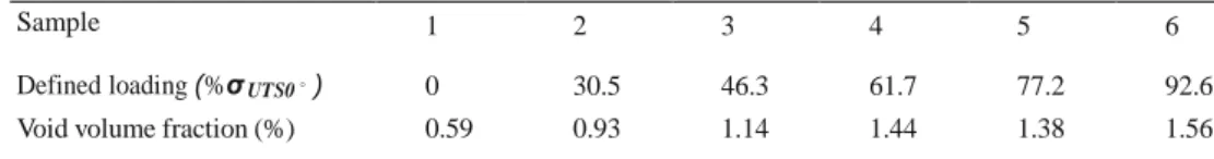
Table 1 Samples with their defined tensile loading for 0◦ and 45◦ samples configuration as well as their tensile induced damage
Sample 1 2 3 4 5 6
Configuration 0◦ 0◦ 0◦ 0◦ 0◦ 0◦
UTS0 UTS0 UTS0 UTS0 UTS0 0
Sample 7 8 9 10
Configuration 5◦ 45◦ 45◦ 45◦
Defined loading 0%σ ◦ 30.5%σ ◦ 61.1%σ ◦ 91.6%σ ◦
Strain 0 0.021 0.082 0.162
Fig. 7 Preliminary C-scan results on 2/2 twill weave fabric reinforced polyamide composite previously loaded in tension with different amplitude. a Samples in 0◦ configuration; b Samples in 45◦ configuration. For the latter, besides the large damage zones, one can easily distinguish the 45◦ orientation of the yarns
Fig. 8 Principle of the X-ray micro computed tomography techniques
[22]
The matrix and the fibers of the composite are character- ized by distinctive values of X-ray absorption. Hence, they can be easily separated on a grey level map. Air cannot signifi- cantly absorb X-ray. Consequently, the voids cannot be easily observed inside the composite samples, however during the image 3D-reconstruction, the voids appear as completely black volumes. A median filtering was first applied to the raw results to reduce the amount of noise in the images. A despeckle filter was then applied to remove the main part of the remaining interference noise. The different reconstruc- tions were then segmented in three classes (void, matrix and fibers) using a grayscale thresholding. The Avizo software segmentation enables an accurate estimation of the volume fraction of each of the three phases. Figure 9 illustrates an
example of a 3D reconstruction of the considered composite material containing an initial porosity.
Prior to a discussion on the evolution of void volume frac- tion, it must be emphasized that the damage mechanisms have been observed for both considered orientations of samples. A characteristic length of the different damage mechanisms was also determined. Those data are critical to understand the damage scheme of the studied material and to validate the results from the ultrasonic study.
3.2 Damage Mechanisms
3.2.1 Sets of Samples Oriented at 0◦ from the Warp Direction
Some examples of damage mechanisms observed for samples in the 0◦ configuration are illustrated in Fig. 10. For tensile tests along the warp fiber axis, the main damage mechanisms observed were the formation of cracks near the end of the yarns (Fig. 10b, c, d), and transverse cracks inside the yarns (Fig. 10a, c), for example). Some longitudinal cracks that follow the transverse yarns very locally in the last step of
damage were also observed (Fig. 10d). As the loading level
increased, the number and the size of defects (cracks and voids) increased too (Tables 3, 4).
The crack inside the yarns has a characteristic thickness of 20 μm, which of the order of magnitude of the size of the fibers. Indeed, it is worth noting that those cracks are caused by fiber/matrix debonding, which propagates perpendicu- larly to the loading direction from one fiber to another. The cracks at the extremities of the yarn have a typical thickness
Table 2 X-ray mCT acquisition parameters
Detector resolution Exposure Voltage Voxel size Focus to detector (FDD) Focus to object distance (FOD)
Sample 1 2 3 4 5 6
Defined loading (%σ UTS0◦ ) 0 30.5 46.3 61.7 77.2 92.6
Void volume fraction (%) 0.59 0.93 1.14 1.44 1.38 1.56
Fig. 9 a As received
mesostructure of the 2/2 twill weave fabric composite obtained by 3D reconstruction prior to mechanical loading. b Initial voids and
process-induced defects are represented by light color and their content is estimated using Avizo software segmentation
(about 0.6% volume)
(a)
(b)
Fig. 10 Three main damage mechanisms identified for 0◦ sample configuration under tension loading. These main mechanisms consist in cracks near the extremities of the yarns, transverse cracks in yarns and longitudinal cracks
Table 3 Void volume fraction
of the tested samples oriented at 0◦ from warp direction
Table 4 Void volume fraction of the tested samples oriented at 0◦ from warp direction
Sample 7 8 9 10
Defined loading (%σ UTS45◦ ) 0 30.5 61.1 91.6 Void volume fraction (%) 0.59 1.69 3.04 5.51
of 50 μm for the highest damaged samples. These longitudi-
nal cracks can then propagate along the warp yarns as shown in Fig. 10d.
3.2.2 Sets of Samples Oriented at 45◦ from the Warp Direction
For samples in the 45◦ configuration, all the observed mech- anisms are shown in Fig. 11. Firstly, cracks at the extremities of yarns (visible in Fig. 11a) as well as cracks along the yarns were observed in Fig. 11a, b. On the 91.6% σ UTS45◦ loaded sample many local fiber breakages were also observed, some of them were already visible in Fig. 11c for the sample tested at 61.1% σ UTS45◦ . Those defects were observed around the central region of the sample, along the loading direction, especially near the edges. In Fig. 11d, some micro buckling
Fig. 11 The different damage mechanisms that appear when a sample in the 45◦ configuration is submitted to tension. These mechanisms consist in transverse cracks, cracks at the extremities of the yarns, fiber breakage, fiber buckling and yarns pseudo-delamination due to the propagation of the longitudinal cracks
of fibers was noted, more notably in the sample loaded at the highest stress level. This is due to the reorientation of fibers during the loading test. Indeed, as the load increases the angle between the fibers tends to decrease but when the tension is interrupted, the fibers cannot return to their orig- inal position because of the section reduction caused by the Poisson effect. This effect of the fibers’ reorientation during off-axis loading was also observed by Vieille and Taleb [23] among others. Pseudo-delamination also appeared locally
after roughly 60.1% σ UTS45◦ of loading in some specimen,
as visible in Fig. 11e. It was propagated inside a yarn and followed the fiber orientation until it reached the location where the weft and warp yarns were intertwined together. When the stress level continued to increase, the crack turned and started propagating along the direction of the other yarn.
It was noticed that the pseudo delamination and fiber buck- ling were the most important damage mechanisms during this study. These mechanisms are actually the only ones that were detected by the ultrasonic C-scan method described in Sect.
2. They both had a characteristic length of 200 μm.
3.3 Micro Computed Tomography Based Void
Volume Fraction Estimation
As previously mentioned, a grey level thresholding, was performed on all the X-ray mCT 3D reconstructions. The evolution of void volume fraction was therefore evaluated. Indeed, the increase of void volume fraction can often be used as a good indicator of damage evolution [24,25].
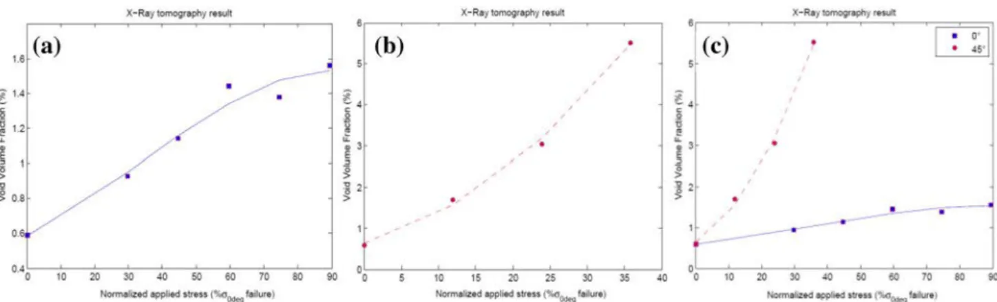
The evolution of the void volume fraction is plotted for both orientations in Fig. 12. The experimental data 0◦ and 45◦ configurations are plotted as function of the stress to failure of the 0◦ sample (respectively Fig. 12a, b). The Fig.
12c allows an easy comparison of the two results.
The void volume fraction clearly increased with the ten- sion loading level for both considered orientations. However, a higher growth of damage in the set of samples oriented at 45◦ from warp direction was observed. In fact, for the sam-ples oriented at 0◦ and loaded at 92.6%σ UTS0◦ , a void volume fraction of 1.56% was measured as it can be seen on the mCT-
3D reconstruction in Fig. 13. On the other hand, as shown
in Fig. 14, for the sample tested at 45◦ for a stress level of 91.6%σ UTS45◦ , the estimated volume void content was about 5.51%. These results are in agreement with the difference in terms of the behavior between the two sample’s orientations discussed in Sect. 2. Indeed, the overall response of the 45◦ samples was more ductile compared to the behavior of a sample tested at 0◦, which exhibited a linear elastic brittle behavior.
The evolution of the void volume fraction as a function of the applied stress level (Fig. 12c) exhibited a similar increase as the evolution of the macroscopic damage estimated from the Young’s modulus reduction plotted in Fig. 6. Accord- ingly, these two quantitative estimations of the damage state, namely void volume content and Young’s modulus reduction will be two actual measurements of the damage that validate the proposed new damage indicators.
Qualitatively, Fig. 13b shows a clear preferred orientation of the damage accumulation, which is perpendicular to the
Fig. 12 Evolution of void volume fraction for a 0◦ and b 45◦ configuration of sample with increasing loading. In c data of both configurations are plotted for comparison purpose
Fig. 13 mCT-3D reconstructions of composite samples in the 0◦ configuration respectively a before and b after tensile loading at a stress level of 92.6%σUTS0◦
Fig. 14 mCT-3D reconstructions of composite samples in the 45◦ configuration respectively a before and b after tensil loading at a stress level of 91.6%σUTS0◦
tension loading direction for the samples oriented along the warp direction (0◦). In the case of the 45◦ samples, the cracks grow along the two yarns direction as visible in the Fig. 14b.
It is worth noting that the estimation of void volume frac- tion and the observation of the damage mechanisms were performed after unloading to zero force (elastic release).
e
Ci j kl nk n j − ρ V 2 i j
Therefore, some of the opened cracks could be partially closed during the unloading and hence cannot be observed. Consequently, the actual void volume content may be to some extent higher than what was measured in the present study. This is especially the case for the 0◦ configuration samples.
For the 45◦ configuration, there is permanent deformation
and higher presence of matrix permanent strain at high load- ing levels reduced the cracks closure effect.
4 Stiffness Components Measurements
Various methods based on ultrasonic wave propagation mea- surements can be utilized to detect the damage in composite materials. It was shown in Sect. 2 that the widely used ultra- sonic C-scan imaging technique may be inefficient to detect the early damage stages for the composite samples oriented at 0◦ and 45◦. As a first approach, a measurement of stiffness components using wave velocity propagation was considered in this section to measure the damage evolution. This stiff- ness components measurement method is described in the first sub-section. Results on samples oriented at 0◦ and 45◦ from warp direction are then presented in further sub-sections and compared. Because of the samples’ low thickness, guided waves propagation is considered for some of the measured signals, further below called plane 1–2; Whereas bulk waves
one can find three different theoretical bulk wave modes: Quasi-Longitudinal, a fast Quasi-Transversal 1 and a slow Quasi-Transversal 2. The QL has a polarization primarily parallel to the direction of n, whereas the QT has a polariza- tion primarily perpendicular to the direction of n.
In order to use this Christoffel’s equation to describe the relation between the velocities of wave propagation inside the material and its stiffness components, these components must not depend on the position inside the material i.e. the material
must be considered as a homogenous medium [26]. There-
fore, the wavelength of the propagating wave must exceed the smallest microstructural features of the undamaged com- posite i.e. the fibers.
From an experimental point of view, the velocity of waves traveling through the sample is obtained by calculating the time delay δt , whether positive or negative measured using an experimental set-up in transmission, visible in Fig. 15b . The latter provides the difference between the time of flight (ToF) of the wave from the emitter to the receiver with the sample and the time of flight of the ultrasonic waves in water (without the sample). So, a first wave time travel measure- ment, without the sample, needs to be performed and used as a reference. Then, the two following equations are used to calculate, respectively, the refraction angle θr and the wave
phase velocity VP:
measurement in transmission are treated for the remaining part of the measured signals, propagating in what we will call, further down, the plane 1–3. The procedure is described
θr = atan 1
sin (θi ) \
cos (θi ) − V0 δt
(3) in the following sub-section. The difference in approach is of
course linked to whether waves propagate as guided waves in the plate or pass through as bulk waves.
Vp = V0 sin (θr )
(4) sin (θi )
4.1 Principle of the Method
The main idea of this method is to measure the velocity of wave propagation at different incidence angles on dif- ferent principal planes. Indeed, it can be shown that, for plane waves, the velocity of wave propagation trough a solid homogenous medium is a function of the stiffness and den- sity of the sample via the following equation, also known as the Christoffel’s equation:
The values are calculated for all considered incidence angles in the plane 1–3 (defined in Fig. 15b).
Because of the dimensions of the samples, measurements of bulk waves in transmission in plane 1–3 were performed but not in the plane 2–3. In order to have sufficient measure- ments to compute at least 7 stiffness constants, additional measurements in the 1–2 plane, (azimuth plane defined in Fig. 15a), were performed. Indeed because of the small thick- ness of the sample, bulk wave measurement in transmission cannot be done since it may cause the sound passing by the (
p δ
\
Ul
= 0 (2) sample and not passing through the sample while rotating
the emitter-receiver couple. As a consequence, the ultrasonic waves propagating in this plane are guided waves that are Where C is the stiffness tensor, n is the vector normal to
the plane of the wave (i.e. n is a vector in the direction of phase propagation), ρ is the material’s density, V is the phase velocity, U is the polarization vector of the mechanical wave and δ is the Kronecker delta symbol.
Depending on the incidence angle, various wave modes may appear. Indeed, by solving the Christoffel equation,
described by other sets of equations.
Indeed, one must be sure that correct descriptors of the acoustic fields inside the plate are considered. For the first arriving pulse passing through the plate along the shortest (straight) path between two transducers facing each other, plane waves are considered responsible of the measured through transmitted pulse. However, guided waves or later
1 2 3 1 1 2 3 2 1 2 3 1 2 2 3 Fig. 15 Schematic
representation of the two planes of interest: a the plane 1–2 or azimuth plane and b the plane 1–3
arriving pulses caused by multiple scattering phenomena can- not be described as plane waves.
In the plane 1–3, considered first, such bulk plane wave approach is acceptable and typically performed, however when guided waves are therefore used in the plane 1–2, we are obliged to use more complicated expressions for guided waves that will be described further below. In fact, guided waves, contrary to the bulk waves described above, are known to be dispersive, and accordingly their phase velocities are function of the frequency and sample thickness, in addition to the material properties. In addition, this dispersive effect induces a phase velocity and a group velocity of the guided waves modes different from one another which affect the interpretation of measured signals.
Although theoretically they can be linked through the same Christoffel’s equation through a plane wave expansion of the acoustic field, experimentally one must take caution as to not confuse one by the other.
Specific experimental procedures must be used if mea- surements of the first or the second velocity is required. Group velocity is usually obtained by ToF measurements on a specific peak in the wave signal for two distances between emitter and receiver (or time-delay measurement). An exper-imental set-up different from the first one presented and
group velocity. However, when the time of arrival is used in the Sect. 5.2, a phase shift is then extract as is and not convert to velocity.
The two experimental set-ups are depicted in Fig. 15. The relation between the frequencies and the group/phase veloc- ities is usually represented on dispersion curves. They were computed for propagation in the considered composite sam- ple along the direction of the fibers using the commercially available Disperse software and are visible in the Fig. 16. The frequency spectrum of every recorded signal is also carefully measured to compare the experimental results with numeri- cal dispersion curves.
Because guided waves propagation along off-principles planes will be considered, the guided wave equations, in explicit format, are needed to be given for a monoclinic stiff- ness tensor. The latter is obtained with a rotation along the axis 3 at a chosen angle of the orthotropic stiffness matrix. In this case, the equations of motion are defined with the following systems of equations. Please note that for more details about the guided waves characteristic equations the reader can refer to the book of Nayfeh [29].
∂2u ∂2u ∂2u
depicted in Fig. 15a is used for acquiring the phase velocities
C11 1 + C44 1 + C55 1
in the plane 1–2. This set-up in immersion using two trans-ducers in pitch-catch, both at a chosen incidence/reflection
∂ x 2 ∂2u 1 ∂ x 2 ∂2u 2 ∂ x 2 ∂2u 2 ∂2u2
angle, can be used to measure the phase velocities [27,28]. The phase velocities VLWP, in the plane of the plate, for Lamb
+ 2C14
∂ x ∂ x + C14
∂ x 2 + C24∂ x 2 + C56 ∂ x 2
waves, are then obtained with the use of the Snell’s law with
θr = 90◦ i.e. equation (4) transforms into: (C12 + C44) ∂
2u 2 ∂ x1∂ x2 + (C13 + C55) ∂ 2u 3 ∂ x1∂ x3 V V0 (5) Lwp = sin (θ ) ∂2u 3 + (C34 + C56) ∂ x ∂ x ∂2u 1 = ∂t 2 (6) i C14 ∂2u 1 ∂ x 2 + C24∂ 2u 1 ∂ x 2 + C56∂ 2u 1 ∂ x 2
For each azimuthal direction of propagation (ψ) in the 1–
2 plane, the incidence angle is adjusted in order to find the same guided wave mode at every acquisition. If the time of
+ (C12 + C44) ∂ 2u 2 ∂ x1∂ x2 + C 44∂ 2u 2 ∂ x 2 + C22 ∂2u 2 ∂ x 2
3 1 2 1 3 linked to the ∂2u2 +C66 ∂ x 2 ∂2u 2 + 2C24 ∂ x ∂ x ∂2u 3 + (C34 + C56) ∂ x ∂ x
2 1 2 1 1 1 3 3 3 3 2 2
Fig. 16 Dispersion curves computed with the Disperse software for guided wave propagation in a 1.53mm thick studied composite along the fibers
direction. a Phase velocities, b group velocities
∂2u 3 + (C23 + C66) ∂ x ∂ x ∂2u 1 ∂2u 1 = ∂t 2 (7) ∂2u 1 And D1q = C13 + C34 Vq + C33αq Wq (C13 + C55) ∂ x ∂ x + (C34 + C56) ∂ x ∂ x D2q = C55(αq + Wq) + C56αq Wq ∂2u 2 + (C34 + C56) ∂ x ∂ x ∂2u 2 + (C23 + C66) ∂ x ∂ x D3q = C56 (αq+ Wq) + C66αq Wq (12) ∂2u 3 + C55 ∂ x 2 ∂2u 3 + C66 ∂ x 2 ∂2u 3 + C33 ∂ x 2
The amplitude ratio Vq and Wq are given by 1 ∂2u 3 2 3 ∂2u 3 V U2q q = U1q and W U3q q = U1q (13) + 2C56 ∂ x ∂ x = ∂t 2 (8)
An overdetermined minimization problem can then be Based on those wave equations the following guided waves
characteristic equations can consequently be obtained:
A = D11 G1 tan (γ α1) − D13 G3 tan (γ α3)
defined. This problem is classically solved by considering a least squares method approach and using a Levenberg- Marquardt algorithm. The stiffness components can be obtained by minimizing the functional F (Ci j ) defined as: + D15 G5 tan (γ α5) = 0;
for the antisymmetric modes
(9 ) F (Ci j ) = [Vex p − Vnum (Ci j ) 2 ] , n S = D11 G1 cot (γ α1) − D13 G3 cot (γ α3) + D15 G5 cot (γ α5) = 0;
for the symmetric modes (10)
wi t h n : t he number o f ex per i ment al velocities
(14)
αq;q=1,3,5 being the solution of the wave equations when the
displacement field is of the forms u j = U j ei ξ (x1+αx3−ct ).
Here U j is the wave amplitude, c is the guided wave phase
velocity, ξ is the wavenumber and γ = ξ d/2 = π fd/c where d is the sample’s thickness and f the wave frequency.
Finally Gi and Diq are given by: G1 = D23 D35 − D33 D25
G2 = D21 D35 − D31 D25
The numerical velocities are determined by solving the
Christoffel equation and the guided waves
characteristic equations for a given set of Ci j . In order
to avoid finding a local minimum solution, it is important to initiate the algo- rithm with a first guess of Ci j that is
relatively close to the real solution.
In this paper, the initialization values of the algorithm are calculated by periodic homogenization computation [30], they are indicated in Table 5. The values of identified stiff- ness components depend on this initial guess but also on the number of experimental velocities considered and the num- ber of principal planes investigated. Therefore it is necessary
∂ F (C i j ) m
Table 5 Comparison between numerical and experimental results of the stiffness constants for undamaged glass fiber reinforced woven composite
C11 C12 C13 C22 C23 C33 C44 C55 C66
Numerical (periodic homogenization) 20 2.1 1.5 20 1.5 4.5 2.3 1.3 1.3
Experimental 22.21 (0.2) 2.57 (0.15) 1.41 (0.76) 21.81 (0.08) – 4.1 (0.07) 2.33 (0.09) 1.58 (0.21) – The numbers between parentheses are the confidence intervals
Fig. 17 a Emitted pulse signal and spectrum b for a 2.25 MHz center frequency transducer. The experimentally mesured center frequency is about
2.1 MHz
to estimate a confidence interval, ci(i), for each component of the identified stiffness matrix. It was proposed by Audoin et al. [31] to use the covariance matrix φ to obtain statistical information of the deviation from the analytical solutions for each stiffness component. This covariance matrix is calcu- lated as:
rt ∗ r t 1
to satisfy the homogenous media hypothesis. The shape and the spectrum of the emitted pulse are represented at Fig. 17.
4.2 Application to Sets of Samples Oriented at 0
◦from the Warp Direction
The composite is considered as orthotropic prior to loading and remains so even after the damage induced by the tensile
φ = n− ∗ ([J] ∗ [J])− (15) loading. The elastic linear behavior of the composite can be
described using nine stiffness components. However,
con-where: [J] = ∂C
i j is the Jacobian matrix, r is the vector
sidering the dimensions of the sample, only measurements in two principal planes were performed as illustrated in Fig. of the residual values i.e. the functional evaluated with the
identified solution, n is the number of experimental velocities and m is the number of stiffness parameters to be identified.
The values of confidence interval can then be extracted from the diagonal terms of the covariance matrix.
ci (i ) = jφ i i (16)
The acquisitions were carried out using a customer-designed five axes immersion scanner fabricated by Inspection Tech-
nology Europe BV. The pulses were emitted by the dual
pulser-receiver DPR500 made by JSR ultrasonics. The exper- imental data were acquired with Winspect software and were post-processed with Matlab. An immersion Panasonic trans- ducer with a central frequency of 2.25 MHz was used in order
15. These measurements only permitted obtaining seven out
of nine stiffness components. It was observed that along the plane 1–3, quasi longitudinal and quasi transversal mode 1 can be measured. For the plane 1–2, on which guided waves propagate, the frequency and phase velocity of the trans- mitted signal was measured. Consequently, after comparison with the dispersion curves in Fig. 16, the mode S2 was prop- agating in the composite.
Before running the optimization procedure for obtaining the stiffness constants, a computation of the expected velocity as a function of the incidence angle was performed. The quasi longitudinal, the quasi transversal 1 and the quasi transversal 2 modes propagated in the 1-3 principle plane were calculated for a refraction angle ranging from 0 to 90◦. This computa-tion was based on the stiffness matrix obtained by periodic
Fig. 18 Comparison of numerically and experimentally determined propagation wave velocities. The experimental values are represented by points
whereas numerical values are represented in continuous line. a Plane 1–3; b Plane 1–2 or azimuth plane
Fig. 19 Evolution of seven of the stiffness constants, function of the tensile stress, with the increase of the loading for the 0◦ configuration of sample with their respective confidence interval
homogenization (Table 5). The computed velocities were compared to those obtained experimentally for the undam- aged sample. The same calculation was made for Lamb wave propagation in the 1-2 planes, more particularly for the S2 mode. The comparison of experimental and analytical veloc- ities of wave propagation is illustrated in Fig. 18. It confirms that the mode experimentally measured corresponds to the actual wave mode that was assumed to propagate in the com- posite material.
For the undamaged sample oriented along the warp direc- tion (0◦), the experimental stiffness constants were close
to the numerically obtained results as observed in Table 5. The evolution of the stiffness constants is plotted in the Fig.
19 with their respective confidence interval. Furthermore, it was noticed that the global evolution of the stiffness compo- nents was close to the results discussed by Hufenbach et al. [9]. An important decrease of the components C11 and C13
almost no change of C33, C22 and C44 compared to the other
stiffness components is remarked (Fig. 19).
One can then conclude that the components depending on the loading direction (direction 1), namely C11 and C13 were
more affected by the damage. The component C12 was also
impacted by the damage but at a lower extent.
4.3 Application to Sets of Samples Oriented at 45
◦from the Warp Direction
In the 45◦ configurations, another propagation plane, named X-3 is considered (defined in Fig. 20). The latter is oriented at 45◦ from the plane 1–3 used in the 0◦ configuration. Indeed, when the sample is oriented at 45◦ from the warp direction, the axis of the sample will correspond to the axis of the plane X-3. The different planes of propagation are illustrated in the Fig. 20. The X-3 plane is not a principal plane of the compos- ite but remains an axis of symmetry in its undamaged state. The same procedure can then be applied. However, when sub-mitted to tension at 45◦ from the warp direction, the damage induced in the sample can introduce loss in elastic symmetry. This can be provoked by the fiber’s reorientations or unex- pected micro cracks perpendicular to the loading direction; even though the Fig. 14b indicates that the majority of the damage is appearing along the two fiber axis (i.e. −/ + 45◦). Therefore, to describe the elastic behavior of the samples oriented at 45◦ with respect to the warp direction, thirteen stiffness components are necessary. The Christoffel equa- tion is consequently modified by considering C56, C14, C24
and C34components for the stiffness tensor. However, ultra-
sonic measurements in four planes are needed to have a good estimation of these thirteen stiffness components. Some non- negligible errors may result from this limitation in the number of measurements.
The evolution of the stiffness components is plotted in Fig.
21 with their respective confidence interval. During the first steps of the loading, the components that are a function of the loading direction (especially C11 and C13) did not change at
Fig. 20 Schematic representation of the different propagation planes
of ultrasonic waves. For samples in the 0◦ configurations, the planes 1–3 and 1–2 were used. For the samples in the 45◦ configuration, the plane X-3 and 1–2 (or azimuth plane) were used
all, but they dropped drastically after 61.1%σ UTS45◦ . The
shear components C44 and C12 were of course impacted
from the beginning of the test. The components C33 and C55
did not really change during the tensile tests. This led to a very different damage behavior compared to the other sam- ple configurations. Some minor changes were observed for the C56, C14, C24 and C34 components. However, the con-
fidence interval was very large when compared to the other stiffness components. This is explained by the lack of mea- surement in two additional planes as mentioned earlier. The major impact from the loading on the shearing components was clearly detected with the present method. Furthermore, this was in agreement with the damage mechanisms observed in the previous section. Indeed, it is worth recalling that the fiber buckling was caused by the reorientation of the fibers which was induced by important local shearing in the meso- structure.
This method can be used to obtain non-destructively the evolution of the stiffness components on a structure sub- mitted to various complex solicitations schemes without performing post-loading tensile tests. This is a significance help for non-destructive damage evaluation.
In the present ultrasonic study, a complete 3D characteri- zation of the stiffness tensor for different damage states was obtained via the velocity of wave propagation through the composite material. An anisotropic evolution of damage dif- ferent from one another was observed for each of the both samples configurations. In addition, the sensitivity of the cho- sen method to detect and quantify different damage scheme was verified. However, it is necessary to note the influence of cracks closed effect that may reduce the amount of damage that can be efficiently quantify. Even if X-ray tomography results indicated the presence of an increasing amount of defects, the stiffness reduction measurements in the present study were only representative of the cracks that remain open after unloading to zero force. As mentioned earlier, the 0◦ configuration might be concerned by this effect at a higher extent than the 45◦ configurations.
It is clear that this leads to an excessive amount of infor- mation that may be difficult to analyze quickly in terms of global damage state. For this reason, two damage indicators are considered in the next section to provide information that could be more easily interpreted in terms of global damage state of a sample.
5 Proposition of New Ultrasound Based
Damage Indicators
In the previous section it was shown that damage growth can be detected and quantified via measurement of wave veloc- ities. This allowed obtaining an almost complete stiffness tensor for each sample. However, it still remains difficult to
/
Fig. 21 Evolution of seven of the stiffness constants with the increase of the applied stress level for different 45◦ configuration of sample with their respective confidence interval
compare the damage state between the different samples. The post processing time to obtain the stiffness constants can be long, so it is interesting to identify a method that can quickly estimate the damage state of the studied material by using the ultrasonic signal directly. In this study, a scalar variable as damage indicator is proposed that is applicable in the indus- try as a practical tool. Usually in the field of ultrasonic, the damage estimation is based on the amplitude attenuation, which is extracted from the raw ultrasonic results (transmit- ted time signals) presented in the previous section. However, it is not really efficient in the present case because it exhibits important oscillations when increasing the loading. There- fore, another damage indicator is necessarily required.
Two damage indicators are presented in this section. The first is the Frobenius norm of the computed stiffness and the second is based on the phase angle shift between wave signals propagated through a damaged and an undamaged sample.
5.1 Frobenius Norm of the Stiffness Tensor Based
Damage Indicator
The Frobenius norm of a tensor is defined as follows:
N f (C) = tr ace (C ∗ C) (17)
With C: the stiffness tensor and C : its conjugate transpose. Taking into account that a proper damage indicator should have a cumulative evolution with the increase of the damage state, the following damage indicator is adopted:
D I1 = abs (N f (C)− N f 0 (C0)) (18)
where N f 0 is the Frobenius norm of an undamaged sample’s
stiffness matrix and C0 is the undamaged sample’s stiffness
matrix. It is recalled that the Frobenius norm actually com- putes the norm of the eigenvector of the matrix C. This is
0
( \
Fig. 22 Evolution of the Frobenius norm of the stiffness matrix for the two configurations of samples a 0◦ and b 4 5◦ function. In c data of both configurations are plotted for comparison purpose
more convenient for this study compared to the quadratic norm or the largest singular value that does not take into account all the components of the eigenvector.
The resulting evolution of the Frobenius norm is plotted, for the configuration 0◦ and 45◦, in the Fig. 22a, b respec-tively. The Fig. 22c with the two configurations is plotted for an easy comparison. A global increase of the indicator for both cases was clearly observed as expected. Furthermore, it was noticed that the indicator increases moderately faster for the 45◦ than for the 0◦ configuration. This aspect is consistent with the different response of the samples when submitted to tension, since the behavior is ductile for 45◦ and brittle for 0◦. The propagation of more cracks in the 45◦ samples was observed by mCT as presented in Sect. 3. The indicator’s value of the 45◦ sample loaded at 91.6%σ UTS45◦ is actually
even higher than the corresponding one for the 0◦ sample loaded at 92.6%σ UTS0◦ .
5.2 Phase Shift Based Damage Indicator
The global shape of the transmitted signal remains mostly unchanged whatever the damage severity at this frequency range as it can be observed in Fig. 23. The phase shift of the signal is therefore considered as a pertinent choice to quan- tify damage state evolution. The non-evolution of the global shape of the signal is induced by the choice of a frequency with which the composite sample is considered as homoge- nous. It is worth mentioning that the time shift corresponds
Fig. 23 Response of ultrasonic signals that propagates through the 1–3
plane, at 0◦ of incidence, of a 0◦ undamaged sample and loaded at a stress level of 150MPa
is possible. This was demonstrated in Sect. 5, and is an impor- tant advantage of the proposed damage indicator. Therefore, as for the previous indicator, the average of all incidence angles of the phase shift was calculated. An increase of the phase shift of the signals induces an increase of the damage indicator. The phase shift indicator is calculated as follow:
nmax
to change in phase or group velocity depending on the case when they are different from each other, as visible in Fig. 16.
1 D I2 = n ∗ 1 abs( ph (n) − ph (n)) , (19) 0
However, the damage indicator that is determined is not an extraction of that velocity but is used as is.
This shift is of course function of the wave propagation
ph (n) =
sp ∗ t
⎛
ph (t , n) (20)
I m (H(t , n)\ ⎞
velocity change that was seen to be effective for quantifying damage, as shown in Sect. 4. In addition, by considering mul- tiple incidence angles, an anisotropic investigation of damage
ph (t , n) = atan ⎝ ⎠ = Im (Log (H(t , n)\\ , Real H(t , n)
Fig. 24 Absolute phase angles evolution with increasing tensile stress to the sample for a 0◦ and b 45◦ configuration of sample. In c data of both configurations are plotted for comparison purpose
Fig. 25 Proposed ultrasonic damage indicators. a Evolution of Frobenius Norm and b Phase shift indicator. Those indicators a plotted for the sets
of samples oriented at 0◦ and 45◦ from the warp direction and function of the normalized applied stress level
with n the considered incidence angle; sp the sampling points of the evaluated signal; H (n) the Hilbert transform of the signal responsefor a given n.
The evolution of this proposed damage indicator for the two samples configurations 0◦ and 45◦ is respectively plotted in Fig. 24a and in Fig. 24b. In the Fig. 24c, the evolu- tion of the damage indicator is plotted for the two samples configurations for comparison purpose. The Fig. 24 points out that the damage measured, using the phase shift indi-cator, for the sample in the 45◦ configuration loaded at stress level of 91.6%σ UTS45◦ reach a level of 0.9. This is
clearly higher than the damage level of 0.3 measured on the sample in the 0◦ configuration and loaded at a stress level of 92.6%σ UTS0◦ . This was also observed with the first
damage indicator based on the Frobenius norm depicted in Fig. 22. It must be emphasized that the proposed dam- age indicator is a relative estimation of the damage with respect to a reference state, which is generally the undamaged state. The experimental procedure and arrangements must be rigorously identical when performing the ultrasonic wave measurements both on the undamaged composite sample and on the damaged one. Indeed, issues with the align- ment of the transducers or the measurement triggering could induce errors in the signals comparison and lead to inaccurate diagnosis.
The two proposed ultrasound based damage indicators
(DI1 and DI2) are respectively plotted in Fig. 25a, b. As illus-
Fig. 26 Damage indicators used as validation tools. a Damage estimated on the elastic modulus reduction and b Void volume fraction. Those
indicators a plotted for the sets of samples oriented at 0◦ and 45◦ from the warp direction and function of the normalized applied stress level
the two sets of samples is very close, until an applied stress ratio of 30%σ UTS0◦ . Beyond this ratio, the Frobenius norm for the 45◦ samples has a faster evolution than that of the 0◦ samples. For the phase shift based indicator, the difference between the two samples orientations is more pronounced. For an applied stress ratio of 12%σ UTS0◦ on the 45◦
sam-ples the value of DI2 reach 0.32 which is close to the highest
value reach for the 0◦ samples. Globally, the two new ultra-sound based damage indicators reveal a higher increase of
the damage state for the samples oriented at 45◦ from the
warp direction.
The estimation of damage based on the elastic modulus
reduction determined in Sect. 2 as well as the void volume
evolution from the X-ray mCT measurements presented in Sect. 3 are respectively plotted in Fig. 26a, b. This figure presents the experimental results used as validation for the new indicators. They indeed exhibit a similar damage evo- lution as function of the applied stress ratio with a higher increase for samples in the 45◦ configurations. It must be noted that the kinetic growth of damage is better predicted by the proposed phase angle shift indicator when compared to those two validation criteria.
6 Concluding Remarks
The anisotropic evolution of damage in polymer based woven composite material is strongly affected by fiber orientation and loading direction. This leads to the appearance of various
damage mechanisms that influence the structural integrity differently. The development of nondestructive evaluation techniques is therefore necessary to determine the possible degradation of composite components on-site in a very appli- cable fashion, in service. These techniques should, however simple, still be sensitive to different damage state evolution schemes.
The present study and results aimed at detecting and quan- tifying the anisotropic evolution of damage with ultrasonic techniques. More specifically polyamide 6.6/6 reinforced with 2/2 twill weave glass fabric samples, preliminary dam- aged by stepwise increase interrupted tensile loading, were used. Two sample configurations were considered: (i) sam-ples oriented at 0◦ and (ii) at 45◦ from the mold flow direction (corresponding to the warp direction). This choice was based on the knowledge of the different behavior between the two orientations, which is from brittle to ductile. The decrease of the elastic modulus was also measured for every considered stress level and used as a first validation result for the pro- posed damage indicators. A higher evolution of damage was observed for the samples oriented at 45◦ from the warp fiber direction.
After highlighting the limitations of classical ultrasonic C-scan imaging to detect early damage state, X-ray mCT has been used to observe the different damage mechanisms such as matrix cracking, micro-buckling and fiber breakage. The void volume fraction was also measured on all considered samples. From the first experimental results, it was observed and confirmed that the largest damage mechanisms appear
on samples in the 45◦ configuration. Those samples exhib-ited also a higher increase of void volume fraction than the samples oriented at 0◦ from the warp direction.
Measurements of the stiffness components on several samples previously damaged at different levels were also performed based on ultrasonic methods. A clear evolution of the stiffness components’ values was observed even for the lowest damage state considered. Both studied samples con- figurations actually exhibit a response that differs from one another. However, it may be difficult to have evident informa- tion on the global damage state from the full stiffness matrix. It was proposed to consider scalar variables, obtained using results from the same ultrasonic method, as damage indi- cators. . It may be true that scalar variables in general lack extensiveness compared with higher dimensional vector or tensor variables, but if what they represent as information is functional as damage indicator then they can be used in the industry. The Frobenius norm of those stiffness matrixes was firstly used as a damage indicator. A damage indicator based on phase angle shift was also proposed to estimate the damage. The information delivered by those two damage indicators showed similarities with the results given by void volume fraction evolution and elastic modulus reduction. In other words, the samples oriented at 45◦ from the warp direc-tion exhibited a higher damage increase with increasing the loading level than the samples in the 0◦ configuration. How-ever, the kinematic increase of damage of the two studied configurations of samples was more successfully evaluated by the phase angle shift damage indicator, if referring to the tensile tests and X-ray mCT results.
The presented ultrasonic method provides an appropriate approach to evaluate the global damage state of a compos- ite material reinforced with a complex fabric. Now that the method is effective under laboratory condition on standard samples, the next step is to validate the method on more complex automotive parts. The proposed method requires adaptations for practical applications. It must be robust in order to provide good repeatability of the measurement to avoid measurement errors that could alter the quality of the damage evaluation, such as wrong ultrasonic transducers’ alignment and measurement triggering. An investigation of the method’s sensitivity with air-coupled transducer could also be considered. Indeed, for more practical applications of the damage evaluation procedure on assembly lines, immer- sion of samples in water should be avoided to improve the method’s applicability.
Acknowledgements The present work was funded by PSA Group and
made in the framework of the OpenLab Materials and Processes. This OpenLab involves PSA Group, The Arts et Metiers ParisTech and Geor- gia Tech Lorraine.
References
1. Volgers, P., Kuhlmann, H., Zhang, Z.: New constitutive model for woven thermoplastic composite materials . In: 2015 SIMULIA Community Conference, pp. 1–13 (2015)
2. Artero-Guerrero, J.A., Pernas-Sánchez, J., López-Puente, J., Varas, D.: Experimental study of the impactor mass effect on the low velocity impact of carbon/epoxy woven laminates. Compos. Struct.
133, 774–781 (2015). https://doi.org/10.1016/j.compstruct.2015. 08.027
3. Malpot, A., Touchard, F., Bergamo, S.: Effect of relative humidity on mechanical properties of a woven thermoplastic composite for automotive application. Polym. Test 48, 160–168 (2015). https:// doi.org/10.1016/j.polymertesting.2015.10.010
4. Atas, C., Sayman, O.: An overall view on impact response of woven fabric composite plates. Compos. Struct. 82, 336–345 (2008). https://doi.org/10.1016/j.compstruct.2007.01.014
5. Golzar, M., Poorzeinolabedin, M.: Prototype fabrication of a com-posite automobile body based on integrated structure. Int. J. Adv. Manuf. Technol. 49, 1037–1045 (2010). https://doi.org/10.1007/ s00170-009-2452-6
6. Markham, M.F.: Measurement of the elastic constants of fibre com-posites by ultrasonics. Comcom-posites 1, 145–149 (1969)
7. Marguères, P., Meraghni, F., Benzeggagh, M.L.: Comparison of stiffness measurements and damage investigation techniques for a fatigued and post-impact fatigued GFRP composite obtained by RTM process. Compos. Part A Appl. Sci. Manuf. 31, 151–163 (2000)
8. Marguères, P., Meraghni, F.: Damage induced anisotropy and stiff-ness reduction evaluation in composite materials using ultrasonic wave transmission. Compos. Part A Appl. Sci. Manuf. 45, 134–144 (2013)
9. Hufenbach, W., Ritschel, T., Böhm, R., Langkamp, A.: Ultrasonic determination of anisotropic damage in fibre and textile reinforced composite materials. In: Conference on Damage in Composite Materials (2006)
10. Baste, S., Aristégui, C.: Induced anisotropy and crack systems ori-entations of a ceramic matrix composite under off-principal axis loading. Mech. Mater. 29, 19–41 (1998). https://doi.org/10.1016/ S0167-6636(98)00003-9
11. Ong, W.H., Rajic, N., Chiu, W.K., Rosalie, C.: Determination of the elastic properties of woven composite panels for Lamb wave stud-ies. Compos. Struct. 141, 24–31 (2016). https://doi.org/10.1016/j. compstruct.2015.12.017
12. Moreno, E., Galarza, N., Rubio, B., Otero, J.A.: Phase velocity method for guided wave measurements in composite plates. Phys. Procedia 63, 54–60 (2015). https://doi.org/10.1016/j.phpro.2015. 03.009
13. Satyanarayan, L., Vander Weide, J.M., Declercq, N.F.: Ultrasonic polar scan imaging of damaged fiber reinforced composites. Mater. Eval. 68, 733–739 (2010)
14. Kersemans, M., Martens, A., Van Den Abeele, K., et al.: Detection and localization of delaminations in thin carbon fiber reinforced composites with the ultrasonic polar scan. J. Nondestruct. Eval.
33, 522–534 (2014). https://doi.org/10.1007/s10921-014-0249-5 15. Karayaka, M., Kurath, P.: Deformation and failure behavior of
woven composite laminates. J. Eng. Mater. Techol. 116, 222–232 (1994)
16. Pandita, S.D., Huysmans, G., Wevers, M., Verpoest, I.: Tensile fatigue behaviour of glass plain-weave fabric composites in on- and off-axis directions. Compos. Part A Appl. Sci. Manuf. 32, 1533– 1539 (2001). https://doi.org/10.1016/S1359-835X(01)00053-7 17. Ladeveze, P., Le, Dantec E.: Damage modelling of the elementary
ply for laminated composites. Compos. Sci. Technol. 43, 257–267 (1992)


![Fig. 8 Principle of the X-ray micro computed tomography techniques [22]](https://thumb-eu.123doks.com/thumbv2/123doknet/7377420.215268/8.892.87.429.356.601/fig-principle-x-ray-micro-computed-tomography-techniques.webp)