Design and validation of a real-time spiking-neural-network decoder for brain–machine interfaces

spiking-neural-network decoder for brain-machine

interfaces

Julie Dethier1,∗_{‡, Paul Nuyujukian}1,2,∗_{, Stephen I. Ryu}3,4_,

Krishna V. Shenoy1,2,5 _{and Kwabena Boahen}1

1_{Department of Bioengineering, Stanford University, Stanford, CA 94305} 2_{Medical Scientist Training Program, Stanford University, Stanford, CA 94305} 3_{Department of Electrical Engineering, Stanford University, Stanford, CA 94305} 4_{Department of Neurosurgery, Palo Alto Medical Foundation, Palo Alto, CA 94301} 5_{Department of Neurobiology, Stanford University, Stanford, CA 94305}

∗_{These authors contributed equally to this work.}

E-mail: jdethier@ulg.ac.be Abstract.

Objective: Cortically-controlled motor prostheses aim to restore functions lost to neurological disease and injury. Several proof of concept demonstrations have shown encouraging results, but barriers to clinical translation still remain. In particular, fully-implanted pure cortical prostheses must satisfy stringent power dissipation constraints so as not to damage cortex.

Approach: One possible solution is to use ultra-low power neuromorphic chips to decode neural signals for these pure cortical implants. The first step is to explore in simulation the feasibility of translating decoding algorithms for brain-machine interface (BMI) applications into spiking neural networks (SNNs).

Main results: Here we demonstrate the validity of the approach by implementing an ‡ Present address: Research Fellow F.R.S.-FNRS, Systmod Unit, Montefiore Institute, University of Liege, Belgium.

existing Kalman-filter-based decoder in a simulated SNN using the Neural Engineering Framework (NEF), a general method for mapping control algorithms onto SNNs. To measure this system’s robustness and generalization, we tested it online in closed-loop BMI experiments with two rhesus monkeys. Across both monkeys, a Kalman filter implemented using a 2000-neuron SNN has comparable performance to that of a Kalman filter implemented using standard floating point techniques.

Significance: These results demonstrate the tractability of SNN implementations of statistical signal processing algorithms on different monkeys and for several tasks, suggesting that a SNN decoder, implemented on a neuromorphic chip, may be a feasible computational platform for low-power fully-implanted prostheses. The validation, robustness, and generalization of this closed-loop decoder system hold promise for SNN implementations on ultra-low power neuromorphic chip using the NEF.

1. Cortically-controlled brain-machine interfaces

1.1. The challenge

Neural motor prostheses aim to help disabled individuals to use computer cursors or robotic limbs by extracting neural signals from the brain and decoding them into

useful control signals (figure 1). Several proof of concept demonstrations have shown

encouraging results. For example, a cortically-controlled motor prosthesis capable of quick, accurate, and robust computer cursor movements by decoding neuronal activity

from 96 channel electrode arrays in monkeys [1]-[4]. This prosthesis, similar to other designs (e.g., [5]), uses a Kalman-filter-based decoder ubiquitous in statistical signal

processing. Such a filter and its variants have demonstrated the highest levels of brain-machine interface (BMI) performance in both humans [5] and monkeys [4]. Even though

successes with non-linear alternative decoder types, such as the unscented Kalman

filter [6] and the population vector algorithm [7], are reported in the literature, this paper focuses on the linear version of the Kalman filter because of its ease of implementation

in steady state and the previous experience with the ReFIT-KF [4].

The lack of low-power electronic circuitry to run decoding algorithms is a major

obstacle to the successful clinical translation of cortical motor prostheses. Fully-implanted pure cortical motor prostheses must meet several criteria: high performance,

robustness, autonomy, biological viability, and a strict power budget. The brain

must not be heated by more than 1◦C to maintain long-term neural cell health. To remain below this limit, a 6 × 6mm2 _{implant may dissipate no more than 10mW [8].}

Conventional processors cannot meet these power constraints. A modern x86 processor consumes approximately 1.8mW [9] just to perform 2D Kalman filtering on a 96 channel

array and operates on the order of Watts, hundreds of times above the upper threshold. This approach will not meet the demands of recording from higher electrode densities

and controlling more degrees of freedom, which require substantially more

computer-intensive decode/control algorithms.

Alternatively, decoding may be performed outside the brain by a wearable computer, allowing the 10mW power budget to be dedicated entirely to recording,

signal preprocessing (amplifying, filtering and digitizing), data preconditioning (syncing, scrambling, and coding), and wireless transmission. For 96 signals sampled at 31.25KHz

and digitized at 10 bits (30Mb/s), a 120nm-CMOS FPGA preconditioner consumes 14mW (scaled from [10]) and a 65nm-CMOS UWB transmitter consumes 0.35mW (8.5

pJ/b) [11]. Assuming a custom preconditioner implementation consumes two orders of

magnitude less power, the preconditioning and transmission power for 96 channels can be reduced to 0.49mW. Extrapolating this number yields 5mW for the 1000 channels

thought to be needed for fast and robust control of a six degree-of-freedom robotic arm [12]. This number can be reduced from 50% to 0.005% of the power budget

if decoding is performed inside the brain. The data transmission rate is reduced from 30Mb/s to 3Kb/s—six signals sampled at 50Hz and digitized at 10bits—with

a proportionate reduction in power. A viable approach if the neural signals can be

decoded using a lot less power than it takes to transmit them in raw form§.

1.2. The neuromorphic alternative

The required power constraints could be met with an innovative ultra-low power

technique: the neuromorphic approach. This approach follows the brain’s organizing

principles and uses large-scale integrated systems containing microelectronic analog circuits to morph neural systems into silicon chips [16, 17]. It combines the best

features of analog and digital circuit design—efficiency and programmability—offering

§ Previous studies suggest that low-noise amplification, analog-to-digital conversion, and spike sorting do not prevent scaling to 1000 channels as they can be performed with a total of 3.5µW per channel if the input-referred noise specification is relaxed from 2.2 to 13µV [13, 14, 15].

potentially greater robustness than either of them [16, 17]. With as little as 50nW

per silicon neuron when spiking at 100Hz [18], these neuromorphic circuits may yield

tremendous power savings over conventional digital solutions because they use an analog approach based on physical operations to perform mathematical computations.

Before designing and fabricating such a dedicated neuromorphic decoding chip, we explored the feasibility of translating decoding algorithms into a spiking neural network

(SNN) in software. Recent studies have highlighted the utility of neural networks for decoding in both off-line [19] and online [20] settings. Similarly, we encouragingly

achieved off-line (open-loop) SNN performance comparable to that of the traditional

floating point implementation [9]. We also realized simulation algorithm enhancements that enable the real-time execution of a 2000-neuron SNN on x86 hardware and reported

preliminary closed-loop results obtained with a single monkey performing a single task [21].

In this study, we extended our preliminary closed-loop tests of the SNN Kalman-filter-based decoder from one to two monkeys and evaluated its performance on multiple

tasks. We first describe the linear filter we used in our system, the Kalman filter already

presented in [1]-[3], and how it functions as a decoder. Next, the Neural Engineering Framework (NEF), the method we use to map this algorithm on to an SNN, is outlined,

together with the optimizations that enabled the software-based SNN to operate in a loop experimental setting. An analysis of the performance achieved in the

closed-loop tests demonstrates the validity of this approach and concludes this paper.

2. Kalman-filter-decoder algorithm

In the 1960’s, Rudolf E. K´alm´an described a new type of linear filter that will be later called the Kalman filter [22]. This filter tracks the state of a dynamical system

Occipital Temporal Frontal Parietal FEF FEF PO sprd Lu IO _sT L Pr iPd spcd OT EC FrO C iA sA spA IP S1 MIP VIP AIP LIP M1 cPMv cPMd SMA preSMA rPMd rPMv 7a 7b Motor prosthesis A B C D E F G H I J K L M N O P Q R S T U V W X Y Z Communication prosthesis Neural signals Control signals Threshold-crossing times Decode algorithm Threshold

Figure 1. System diagram of a BMI. Electronic neural signals are measured from motor regions of the brain, converted to spike trains by detecting threshold-crossings, and translated (decoded) into control signals for a computer or prosthetic arm. Current implementations record neural signals with an implanted silicon microelectrode array, threshold and wirelessly transmit these signals with a battery-powered head-mounted unit, and decode them with a remote desktop computer.

throughout time using a weighted average of two types of information: a value predicted from the output state’s dynamics and a value measured from external observations, both

subject to noise and other inaccuracies. More weight is given to the value with the lower uncertainty as calculated by the Kalman gain, K, which is computed as follows.

The system is modeled by the following set of equations:

xt = Axt−1+ wt (1)

yt = Cxt+ qt (2)

where A is the state matrix modeling the output state’s dynamics, C is the observation matrix, and wtand qtare additive, multivariate Gaussian noise sources that are modeled

with wt ∼ N (0, W ) and qt ∼ N (0, Q). The model provides an estimate of the output

the noisy observations at time t to arrive at a final estimate:

xt = (I − KC)Axt−1+ Kyt= Mxxt−1+ Myyt (3)

where K = (I + WCQ−1C)−1WCTQ−1 is the steady-state formulation of the Kalman

gain. Mx and My are the two matrices in the steady-state Kalman-filter-update

equations. It is this steady-state equation that we implemented in the SNN using the

NEF.

For neural prosthetic applications [1], the system’s state vector, xt, was

the kinematic state of the cursor: xt = [posxt, pos y

t, poszt, velxt, vel y

t, veltz] and the

measurement vector, yt, was the neural spike rate (binned threshold-crossing counts

of measured neural potential) of the recorded neurons. For our system, the state vector

was limited to velocities in two directions (xt = [velxt, vel y

t]) to limit the amount of

computational resources required (Kim et al. [5] compare position and velocity decoders

and finds that velocity decoders tend to outperform position decoders in tetraplegic

patients). This velocity was integrated to yield the 2D position. The bin width of the decoder, a tradeoff between rapidity and accuracy [1], was 50ms long. To allow for a

fixed offset compensation (baseline firing rates), a constant 1 was added to the state vector: xt = [velxt, vel

y

t, 1]. The neural spike rate observations yt came from 96-channel

silicon electrode arrays implanted in areas of cortex responsible for arm movement (M1 and PMd).

The model parameters (A, C, W and Q) were fit by correlating recorded

neural signals and measured arm kinematics, obtained during training trials. Arm measurements were captured by a Polaris Optical Measurement System (Northern

Digital Inc), with a passive reflective bead tied to the tip of the monkey’s finger. The measurements were sampled at 60Hz and were plotted directly to the screen. For our

Cha nn el 10 15 0 0.5 -0.5 -0.5 0 0.5 Time (s) 0 5 y-ve loc ity (m /s ) x-ve loc ity (m /s ) 0 12 -12 -12 0 12 Trials: 0322 - 0337 x-position (cm) y-pos it ion (c m ) (A) (B) (C)

Figure 2. Neural and kinematic measurements (monkey J, 2011-04-16, 16 continuous trials) used to fit the Kalman-filter model. (A) The 192 channel recordings that were fed as input to fit the Kalman-filter matrices (grayscale refers to the number of threshold crossings observed in each 50ms bin, black saturation at 4 spikes/bin). (B) Hand x- and y-velocity measurements that were correlated with the neural data to obtain the Kalman-filter matrices. (C) Hand position kinematics of the 16 continuous trials recorded using a Polaris Optical Measurement System (Northern Digital Inc).

to neural signals recorded under brain control, and that the observed arm kinematics matched the desired neural cursor kinematics. Therefore, the parameters could be fit

from observed arm kinematics (figure 2).

For neuroprosthethic applications, the Kalman filter converges to its steady-state

matrices, Mx and My, rapidly—typically less than 100 iterations [23]. The steady-state

implementation differs from the full Kalman-filter implementation by less than 1% in the first few seconds, for both open-loop and closed-loop systems [23]. The steady-state

update equations decrease execution time for typical decoding by approximately a factor seven [23], a critical difference for real-time applications. Thus, efficiency is improved

without any meaningful loss of accuracy.

To map the steady-state version of this linear neural decoder on to an SNN, we

3. Mapping onto spiking neural networks

The SNNs employed in the NEF are composed of highly heterogeneous spiking neurons characterized by a nonlinear multi-dimensional vector-to-spike-rate function—

ai(x(t)) for the ith neuron—with parameters (preferred direction, maximum firing rate,

and x-axis intercept) drawn randomly from a wide distribution (standard deviation

comparable to mean) and with connection strengths programmed to perform the desired

computations. To map control-theory algorithms onto SNNs, three principles—neural representation, transformation, and dynamics—apply [24]-[27].

3.1. Representation

Neural representation is defined by nonlinear encoding of a stimulus, x(t), as a spike

rate, ai(x(t)), combined with optimal weighted linear decoding of ai(x(t)) to recover, in

the stimulus space, an estimate of x(t), ˆx(t) =P

iai(x(t))φxi , where φxi are the optimal

decoding weights.

3.1.1. Nonlinear encoding The nonlinear encoding process is exemplified by the neuron

tuning curve (figure 3 Representation), which captures the overall encoding process from a multi-dimensional stimulus, x(t), to a one-dimensional soma current, Ji(x(t)), and

finally to a firing rate, ai(x(t)):

ai(x(t)) = G(Ji(x(t))), (4)

where G() is the nonlinear function describing firing rate’s dependence on the current’s value. In the case of the leaky integrate-and-fire neuron model (LIF) that we used for

this application, this function G() is given by:

G(Ji(x(t))) = h τref − τRC_{ln (1 − J} th/Ji(x(t))) i−1 , (5)

where Ji is the current entering the soma of the cell, i indexes the neuron, τref is

the absolute refractory period, τRC _{is the membrane RC time constant, and J} th is

the threshold current. The LIF neuron has two behavioural regimes: sub-threshold and super-threshold. The sub-threshold regime is described by an RC circuit with

time constant τRC. When the sub-threshold soma voltage reaches the threshold, Vth,

the neuron emits a spike δ(t − tn). After this spike, the neuron is reset and rests

for τref seconds before it resumes integrating. Ignoring the soma’s RC time-constant when specifying the SNN’s dynamics is reasonable because the neurons cross threshold

at a rate that is proportional to their input current, which thus sets the spike rate

instantaneously, without any filtering [24].

The conversion from a multi-dimensional stimulus, x(t), to a one-dimensional soma

current, Ji, is performed by assigning to the neuron a preferred direction, ˜φxi, in the

stimulus space and taking the dot-product:

Ji(x(t)) = αi

D

˜

φx_i · x(t)E+ J_ibias, (6)

where αi is a gain or conversion factor, and Jibias is a bias current that accounts for

background activity. In the one-dimensional case, the preferred direction vector reduces to a scalar, either 1 or −1, resulting in a positive or negative slope, respectively (i.e.,

ON neurons that increase their firing rate as the value of the stimulus variable increases and OFF neurons that do the opposite).

3.1.2. Linear decoding The linear decoding process converts spike trains back into a

relevant quantity in the stimulus space. This process is characterized by the synapses’ spike response, h(t) (i.e., post-synaptic current waveform), and the decoding weights,

φx_i, which are found by a least-squares method [24], described next.

of introducing uncertainty into any signal sent by the transmitting neuron. With this

noise term, the transmitted firing rate can be written as ai(x(t)) + ηi. That is, the firing

rate that the receiving neuron actually perceives is the noiseless firing rate, ai(x(t)),

plus some variation introduced into that neuron’s activity by the noise sources, ηi.

The noise sources are modeled by a random variable drawn from a normal distribution. Consequently, the mean square error between the actual stimulus, x(t), and its estimate,

ˆ x(t) =P i(ai(x(t)) + ηi) φxi , can be written as [24]: E = 1 2 D [x(t) − ˆx(t)]2E x,η,t (7) = 1 2 *" x(t) −X i (ai(x(t)) + ηi) φxi #2+ x,η,t (8)

where h·i_x,η denotes integration over the range of x and η, the expected noise. We assume that the noise is independent and has the same variance for each neuron [24],

yielding: E = 1 2 *" x(t) −X i ai(x(t))φxi #2+ x,t + σ2X i (φx_i)2, (9)

where σ2 is the noise variance. This expression is minimized by choosing the decoding weights such that:

φx_i =

N

X

j

Γ−1_ij Υj, (10)

with Γij = hai(x)aj(x)i_x + σ2δij, where δ is the Kronecker delta function, and

Υj = haj(x)xi_x [24]. One consequence of modeling noise in the neural representation

is that the matrix Γ in (10) is invertible despite the use of a highly overcomplete

representation. In a noiseless representation, Γ would be generally singular because, due to the large number of neurons, there would be a high probability of having two

Representation Transformation Dynamics x and ˆx y = Ax x = Ax˙ 0 0.2 -0.2 Encoded signal V el oc ity 0 2 4 6 8 10 -0.2 0 0.2 Time (s) x-velocity(m/s) y-velocity(m/s) A y(t) = A x(t) x(t) ai(t) bj(t) ωji(t) A dt _x(t) x(t)˙ V el oc ity Decoded signal N euron N um be r _{Spike raster} x(t) ai(t) A x → ai(x) and ˆx = Piai(x)φxi x → ai(x) x = h ∗ [A0x] ai(x) = G(αi D ˜ φx i · x E + Jbias i ) bj(A ˆx) = G(Piωjiai(x) + Jjbias) A0 = τ A + I

Figure 3. NEF’s three principles. Top row represents the control-theory level and lower rows the neural level. Representation. Encoded signal, spikes raster, and decoded signal with a population of 200 leaky integrate-and-fire neurons. The neurons’ tuning curves map the encoded signal (x) to spike rates (ai(x)); this

nonlinear transformation is inverted by linear weighted decoding to retrieve the decoded signal ( ˆx). G() is the neurons’ nonlinear current-to-spike-rate function. Transformation. SNN with populations ai(t) and bj(t) representing x(t) and

y(t), respectively, with decoding, transformation, and encoding performed via the feedforward weights ωji = αjD ˜φyj · Aφ

x i

E

. Dynamics. The system’s dynamics is captured in a neurally plausible fashion by replacing integration with the synapses’ spike response, h(t), and replacing the matrix with its neurally plausible equivalent, A0= τ A + I, to compensate.

3.2. Transformation

Neural transformation is a special case of neural representation performed by using alternate decoding weights in the decoding operation. The transformation, f (x(t)),

is mapped directly into transformations of ai(x(t)) by using the appropriate linear

decoders, φf (x(t))_i , to extract the function from the encoded information. For example, y(t) = Ax(t) is represented by the spike rates bj(A ˆx(t)) (figure 3 Transformation),

P

iai(x(t))Aφxi, an alternative linear weighting.

3.3. Dynamics

Neural dynamics brings the first two principles together and adds the time dimension

to the circuit. This principle aims at reuniting the control-theory and neural levels by modifying the matrices to render the system neurally plausible, thereby permitting the

synapses’ spike response, h(t), to capture the system’s dynamics.

For example, in control-theory, an integrator is written ˙x(t) = Ax(t) + By(t) with Laplace transform x(s) = 1/s [Ax(s) + By(s)]. In the neural space, convolution

replaces integration and the system takes the form x(t) = h(t) ∗ [A0x(t) + B0y(t)] and its Laplace transform is x(s) = h(s) [A0x(s) + B0y(s)]. The synapses’ spike response

takes the form h(t) = τ−1e−t/τ where τ is the synaptic time constant, and the transfer function is h(s) = 1/ (1 + sτ ). The two systems are therefore equivalent if A0 = τ A + I

and B0 = τ B, so called neurally plausible matrices (figure 3 Dynamics).

4. Spiking neural network decoder

To implement the Kalman filter in an SNN by applying the NEF, we used the three principles described in the previous section (figure 4). To render the system neurally

plausible as explained in section 3.3, we started from a continuous time (CT) system in

the control-theory space, and we therefore converted (3) from discrete time to CT:

˙

x(t) = MCT_x x(t) + MCT_y y(t) (11)

where MCT

x = (Mx− I) /∆t and MCTy = My/∆t are the CT Kalman matrices and ∆t

is the discrete time step (50ms).

From (11), by applying the dynamics’ principle, we replaced integration with convolution by the synapse’s spike response and the CT matrices with neurally plausible

ones, which yielded:

x(t) = h(t) ∗ (A0x(t) + B0y(t)) , (12)

where A0 = τ MCT

x + I = τ (Mx− I)/∆t + I and B0 = τ MCTy = τ My/∆t.

The jth neuron’s input current (see (6)) was computed from the system’s current state, x(t), which was computed from estimates of the system’s previous state ( ˆx(t) =

P

iai(t)φxi) and current measurements ( ˆy(t) =

P

kbk(t)φyk) using (12). These quantities

were decoded from the firing rates of the corresponding neural populations using the representation principle. This procedure yielded:

Jj(x(t)) = αj D ˜ φx_j · x(t)E+ J_jbias (13) = αj D ˜ φx_j · h(t) ∗ (A0x(t) + Bˆ 0y(t))ˆ E+ J_jbias (14) = αj * ˜ φx_j · h(t) ∗ A0X i ai(t)φxi + B 0X k bk(t)φyk !+ + J_jbias (15)

This last equation can be written in a neural network form (figure 4):

Jj(x(t)) = h(t) ∗ X i ωjiai(t) + X k ωjkbk(t) ! + J_jbias (16) where ωji= αj D ˜ φx_j · A0_φx i E and ωjk = αj D ˜ φx_j · B0_φy k E

are the recurrent and feedforward weights, respectively.

4.1. Efficient implementation

A software SNN implementation involves two distinct steps [21]: network creation

and real-time execution. The network does not need to be created in real-time and therefore has no computational time constraints. However, executing the network has

to be implemented efficiently for successful deployment in closed-loop experimental

settings. To speed-up the simulation, we exploited the NEF mapping between the high-dimensional neural space and the low-high-dimensional control space. This mapping updated

1 ωji ωjk _a j(t) aj(t) ωji ωjk bk ( t )

Figure 4. SNN implementation of a Kalman-filter-based decoder with populations bk(t) and aj(t) representing y(t) and x(t). Feedforward and recurrent weights, ωjk

and ωji, were determined by B0 and A0, respectively.

neuron interactions circuitously, using the decoding weights φx

j, dynamics matrix A 0_,

and preferred direction vectors ˜φx

j from (15), rather than directly using the recurrent

and feedforward weights in (16). The circuitous approach yielded an almost 50-fold speedup [21], enabling real-time execution of a 2000-neuron network.

Other improvements to the basic SNN consisted of using two one-dimensional integrators instead of a single three-dimensional one, feeding the constant 1 into the

two integrators continuously rather than obtaining it internally through integration, and connecting the 192 neural measurements directly to the recurrent pool of neurons,

without using the bk(t) neurons as an intermediary (figure 4) [9].

4.2. Choice of parameters

Various parameters needed to be set for this network. They are recapitulated in table 1. Neural spike rates were computed in 50ms time-bins and, therefore, the

sum τRC

j + τjref + τjPSC had to be smaller than 50ms, which was indeed the case. It was

Table 1. Model parameters.

Symbol Range Description

max G(Jj(x)) 200-400 Hz Maximum firing rate

G(Jj(x)) = 0 −1 to 1 Normalized x-axis intercept

Jbias

j Satisfies first two Bias current

αj Satisfies first two Gain factor

˜ φx_j ˜ φx_j

= 1 Preferred direction vector σ2 _{0.1 Gaussian noise variance}

τRC j 20 ms RC time constant τref j 1 ms Refractory period τPSC j 20 ms PSC time constant

randomly selected from a wide distribution. Specifically, the preferred direction vectors, ˜

φx

j, were drawn between -1 and 1. The maximum firing rate, max G(Jj(x)), and the

normalized x-axis intercept, G(Jj(x)) = 0, were drawn from a uniform distribution on

[200, 400] Hz and [-1, 1], respectively. The gain and bias current, αj and Jjbias, were

chosen to satisfy these constraints. τRC

j was chosen at 20 ms, close to typical membrane

time constant values, and τref

j was set to 1 ms, again a typical value [26] . The time

constant for the synapses’ spike response dynamics, τPSC

j , was set to 20 ms, dynamics

consistent with post-synaptic currents [26].

Noise was not explicitly added. It arose naturally from the fluctuations produced

by representing a scalar through the filtering of spike trains, which has been shown to have effects similar to Gaussian noise [24]. For the purpose of computing the linear

decoding weights (i.e., Γ), we modeled the resulting noise as Gaussian with a variance of 0.1 [24].

5. Off-line open-loop implementation

We first performed an off-line open-loop validation of our SNN decoder [9] by using

a previously recorded BMI experiment that utilized a standard Kalman filter (SKF)

trained to perform a point-to-point arm movement task in a 3D experimental apparatus

for a juice reward [1]. All animal procedures and experiments were approved by the

Stanford Institutional Animal Care and Use Committee. A 96-electrode silicon array (Blackrock Microsystems) was implanted in the dorsal pre-motor (PMd) and motor (M1)

cortex areas responsible for hand movement as guided by visual cortical landmarks. Array recordings (-4.5× RMS threshold crossing applied to each channel) yielded tuned

activity for the direction of arm movements. For both monkeys (Monkey L and J) the electrode array used in these experiments spanned approximately 4-6 mm of

anterior-posterior distance on the pre-central gyrus associated with primary motor cortex (M1).

Electrical stimulation and/or manual arm palpation further localized the area to the upper shoulder region/muscles (monkey J) and forearm (monkey L). It should be kept

in mind that the border between M1 and the dorsal premotor (PMd) cortex is not sharp neurophysiologically, and it is possible that the anterior aspect of either array could be

within PMd. In addition, for monkey J, we also recorded simultaneously from a second array which is the same as the first array except that it was implanted 1-2 mm anterior

to the first array, and is thus nominally in PMd (see [28], supplementary figure 5, for

an intraoperative photo of the arrays). For the purposes of the current experiments the distinction between these two areas is not of primary importance since both areas have

robust movement-related activity and modulation.

As detailed in [1], a Kalman filter was fit by correlating the observed hand

kinematics with the simultaneously measured neural signals (figure 2). The resulting model was used online to control an on-screen cursor in real time. This model and 500 of

these trials (L20100308) served as the standard against which the SNN implementation’s

performance is compared. Starting with the steady-state Kalman-filter matrices derived from this experiment, we built an SNN using the NEF methodology and simulated it in

Time (s) 0 1 2 3 4 5 −0.2 0 0.2 Time (s) x− ve loc it y (m /s ) 0 1 2 3 4 5 y− v e loc it y (m /s ) 200 neurons - RMS: 21% (A) (B)

Standard Kalman Filter Spiking Neural Network

(C) −0.2 0 0.2 Time (s) 0 1 2 3 4 5 2000 neurons - RMS: 6% 20 000 neurons - RMS: 3% (D) (E) (F)

Figure 5. Comparing the x and y-velocity estimates decoded from 96 recorded cortical spike trains (5s of data) by the SKF (red) and the SNN (blue). Networks with (A and B) 200, (C and D) 2000, and (E and F) 20 000 spiking neurons. Absolute RMS (RMS error normalized by maximum velocity) in indicated above each plot.

Nengo, a freely available software, using the parameter values listed in table 1.

The SNN performed better as we increased the number of neurons (figure 5). For 20 000 neurons, the x and y-velocity decoded from its two 10 000-neuron populations

matched the standard decoder’s prediction to within 3% (RMS error normalized by

maximum velocity) [9]. There was a tradeoff between accuracy and network size. If the network size was decreased to 2000 neurons, the network’s error increased to 6%; an

even bigger decrease to 200 neurons led to an error of 21% [9]. Even with a 6% RMS error at 2000 neurons, we believed that this may provide sufficient accuracy to use in

closed-loop experiments.

6. Online closed-loop performance

These off-line results encouraged us to test our SNN decoder in an online closed-loop setting. Despite the error, we suspected that the monkeys would actively compensate

for any noticeable cursor deviation. Two adult male rhesus macaques (Monkey L and

J) were trained to perform a point-to-point arm movement task in a 3D experimental apparatus for a juice reward using the ReFIT-KF training protocol as detailed in the

Decoder Neural Spikes Cursor Velocity (A) 1 2 3 4 5 6 2cm (B) (C)

Figure 6. Experimental setup and tasks. (A) Data are recorded from silicon electrode arrays implanted in motor regions of cortex of monkeys performing a center-out-and-back or pinball task for juice rewards to one of eight targets with a 500ms hold time. (B) Center-out and back task. (C) Pinball task.

methods section of [4] (figure 6 (A)). Unlike Monkey L who only had one array, Monkey

J had two 96-electrode silicon arrays (Blackrock Microsystems) implanted, one in PMd and the other in M1. The Kalman filter was built as described in prior work [4]. The

resulting models were used in a closed-loop system to control an on-screen cursor in real-time (figure 6 (A), Decoder block) and once again served as the base performance

against which the SNN’s performance was compared.

A 2000-neuron SNN decoder was built using the simulation algorithm enhancements mentioned earlier and simulated on an xPC Target (Mathworks) x86 system (Dell T3400,

Intel Core 2 Duo E8600, 3.33GHz). It ran in closed-loop, replacing the SKF as the decoder block in figure 6 (A). Real-time execution constraints with our hardware limited

the network size to no more than 2000 neurons.

6.1. Center-out and back task

Once the Kalman filter was trained and the SNN was built, we tested the two Kalman filter implementations (SKF and SNN) against each other. Each test was composed of

200 trials of target acquisition on a center-out and back task. The target alternated from the center of the workspace to one of eight peripheral locations chosen at random

the target and holds within the 4 cm square acquisition region for 500 ms during the

alloted 3 seconds. Once a block of 200 trials was completed with one implementation,

the decoder was switched to the other implementation and another block was collected. This ABA block switching was continued until the monkey was satiated and enabled an

accurate comparison of just the relative difference in implementations. This ABA block style experimentation was repeated for at least three days with each monkey.

Success rates were higher than 94% on all blocks for the SNN implementation (94.9% and 99.6% for Monkey L and J, respectively) and 98% for the SKF (98.0%

and 99.7% for Monkey L and J, respectively). Thousands of trials were collected and

analyzed (5235 with Monkey L and 5187 with Monkey J). These reflect only center-out trials, not those that returned to the center from the periphery. The latter were not

included in the analysis because the monkey anticipated the return to the center after navigating out to the periphery and thus initiated movement earlier than when the

target location is unknown. About half of the trials, 2615 (2484), were performed with the SNN for Monkey L (Monkey J) and 2518 (2599) with the SKF. The average time to

acquire the target was moderately slower for the SNN for both monkeys—1067ms vs.

830ms for Monkey L and 871ms vs. 708ms for Monkey J. Around 100 trials under hand control were used as a baseline comparison for each monkey.

Although the speed of both implementations was comparable, as evidenced by the traces being nearly on top of each other up until the first acquire time, the SNN has

more difficulty settling into the target (Figure 8). Whereas the time at which the target was first successfully acquired (average indicated by trace becoming thicker) is

comparable for both BMI implementations, the time at which the target was successfully

last acquired (average indicated by trace’s cutoff) occurs latter for SNN. That is, the monkey spent more time wandering in and out of the acquisition region, before

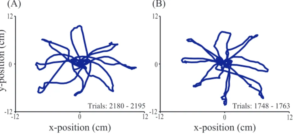
Trials: 1748 - 1763 0 12 -12 -12 0 12 x-position (cm) Trials: 2180 - 2195 -12 0 12 -12 0 12 y-pos it ion (c m ) x-position (cm) (A) (B)

Figure 7. Center-out and back task (monkey J, 2011-04-16). (A) BMI position kinematics of 16 continuous trials for the SKF implementation. (B) BMI position kinematics of 16 continuous trials for the SNN implementation.

0 500 1000

0 5 10

Time after target onset (ms)

Distance to target (cm) 0 500 1000

Hand SNN SKF

(A) (B)

Figure 8. SNN (red) performance compared to SKF (blue) (hand trials are shown for reference (yellow)). The SNN achieves similar results as the SKF implementation. Plot of distance to target vs. time after target onset for different control modalities. The thicker traces represent the average time when the cursor first enters the acceptance window until successfully beginning the 500ms hold time. Results for Monkey L (A) and results for Monkey J (B).

subsequently successfully staying inside it for the required hold time. This longer

dial-in time (dial-indicated by length of thick trace) suggests that the SNN provides less precise control when attempting to stop.

Towards the end of the day’s experiments, the SNN decoder would occasionally

fall to edge of the workspace and the monkey would lose interest in the task. The cursor was reset to the center of the screen so the monkey would continue the block.

center-out trials. The off-line results shown earlier (see figure 5) suggest that this difference

usability, as well as the difference in performance, is a result of the network’s neuron

count, which was limited by the real-time execution capacity of the x86 hardware. These performance issues could be improved by using more neurons, as would be the case in

a neuromorphic chip. Nevertheless, even with only 2000 neurons, the success rate and acquire times of the SNN decoder are comparable to that of the SKF decoder.

6.2. Pinball task

Another important measure when evaluating decoders is generalization and stability. To

test this, we instructed a new pinball task under the SNN decoder. In this task, targets appeared randomly in a 16 cm square workspace without any systematic structure to

target placement (see figure 6 (C)). The monkey received a reward by navigating to the target and holding within the 4cm acquisition region for 500 ms. Successfully performing

this task highlights the SNN decoder’s generalization. There was no block structure in

this set of experiments. The monkeys were started on this task and were allowed to run continuously without interruption until satiated. Successfully performing this task

highlights the SNN decoder’s stability over an extended period of time.

Both monkeys sustained performance at around 40 targets per minute for over an

hour on the pinball task (figure 9). On the day tested, monkey L lost interest in the task after approximately 61 minutes and monkey J after approximately 85 minutes. The

sustained performance of the SNN decoder across both monkeys in a more generalized

task demonstrates the robust performance of the system over uninterrupted periods, suggesting that the decoder is capable of sustained performance across long stretches

of time. This performance is comparable to the hit rate and session duration achieved under hand control [20].

0 30 60 90 0 20 40 60 Time (minutes)

Hit Rate (min

−1

)

0 30 60 90

(A) (B)

Figure 9. Sustained performance plots for both monkeys using the SNN decoder under the pinball task. The sharp falloff represents a loss of interest in the task, which occurred when the monkey was satiated. Results for Monkey L (A) and for Monkey J (B).

7. Conclusions and future work

The SNN decoder’s performance was comparable to that produced by a SKF. The

2000-neuron network had success rates higher than 94% on all blocks but took moderately longer to hold the cursor still over targets. Performance was sustainable for at

least an hour under a generalized acquisition task. As the Kalman filter and its variants are the state-of-the-art in cortically-controlled motor prostheses [1]-[5], these

simulations increase confidence that similar levels of performance can be attained with a

neuromorphic chip, which can potentially overcome the power constraints set by clinical applications. A neuromorphic chip could implement a 10 000-neuron network while

dissipating a fraction of a milliwatt, likely increasing the performance of the system compared to the simulated SNN shown here.

This demonstration is an important proof-of-concept that highlights the feasibility of mapping existing control theory algorithms onto SNNs for BMI applications. For

BMIs to gain widespread clinical deployment, they must packaged in low-power,

completely implantable, wireless systems. The computational demands of BMI decoding are high, and thus present a problem for low-power applications. Implementing the SNN

complex and demanding computations at a fraction of the power draw of conventional

processors. Translating the SNN from software to ultra-low-power neuromorphic chips is

the next step in the development of a fully-implantable neuromorphic chip for cortical prosthetic applications. Currently, we are exploring this mapping with Neurogrid, a

hardware platform with sixteen programmable neuromorphic chips that can simulate up to a million spiking neurons in real-time [17].

Acknowledgments

The authors would like to thank the support of Joline M Fan and Jonathan C Kao

for assistance in collecting monkey data; Mackenzie Mazariegos, John Aguayo, Clare Sherman, and Erica Morgan for veterinary care; Kimberly Chin, Sandra Eisensee,

Evelyn Castaneda, and Beverly Davis for administrative support. We also thank Chris Eliasmith and Terry Stewart for valuable help with Nengo.

This work was supported in part by the BAEF and F.R.S-FNRS (J. Dethier),

Stanford NIH Medical Scientist Training Program (MSTP) and Soros Fellowship (P. Nuyujukian), DARPA Revolutionizing Prosthetics program (N66001-06-C-8005,

K. V. Shenoy), two NIH Director’s Pioneer Awards (DP1-OD006409, K. V. Shenoy; DPI-OD000965, K. Boahen), and an NIH/NINDS Transformative Research Award

(R01NS076460, K. Boahen).

References

[1] Gilja V 2010 Towards clinically viable neural prosthetic systems , (Ph.D. Thesis, Department of Computer Science, Stanford University) pp 19–22 and pp 57–73

[2] Nuyujukian P, Gilja V, Chestek C A, Cunningham J P, Fan J M, Yu B M, Ryu S I and Shenoy K V 2010 Generalization and robustness of a continuous cortically-controlled prosthesis enabled by feedback control design Society for Neuroscience 2010 (San Diego) Program No. 20.7.

[3] Gilja V, Chestek C A, Diester I, Henderson J M, Deisseroth K and Shenoy K V 2011 Challenges and opportunities for next-generation intra-cortically based neural prostheses IEEE Trans. Biomed. Eng. 58(7) 1891–9

[4] Gilja V, Nuyujukian P, Chestek C A, Cunningham J P, Yu B M, Fan J M, Churchland M M, Kaufman M T, Kao J C, Ryu S I and Shenoy K 2012 A high performance neural prosthesis enabled by control algorithm design Nature Neurosci. 15 1752–7

[5] Kim S P, Simeral J D, Hochberg L R, Donoghue J P and Black M J 2008 Neural control of computer cursor velocity by decoding motor cortical spiking activity in humans with tetraplegia J. Neural Eng. 5(4) 455–76

[6] Li Z, ODoherty J E, Hanson T L, Lebedev M A, Henriquez C S, Nicolelis M A L 2009 Unscented Kalman filter for brain-machine interfaces PLoS One 4(7) e6243

[7] Chase S M, Kass R E, Schwartz A B 2012 Behavioral and neural correlates of visuomotor adaptation observed through a brain-computer interface in primary motor cortex J. Neurophysiol. 108(2) 624–44

[8] Kim S, Tathireddy P, Normann R A and Solzbacher F 2007 Thermal impact of an active 3-D microelectrode array implanted in the brain IEEE Trans. Neural Syst. Rehabil. Eng. 15(4) 493–501

[9] Dethier J, Gilja V, Nuyujukian P, Elassaad S A, Shenoy K V and Boahen K 2011 Spiking neural network decoder for brain-machine interfaces Proc. of the 5th Int. IEEE EMBS Conf. on Neural Engineering 2011 (Cancun, Mexico) pp 396–9

[10] Miranda H, Gilja V, Chestek C A, Shenoy K V and Meng T H 2010 HermesD: A high-rate long-range wireless transmission system for simultaneous multichannel neural recording applications IEEE Trans. Biomed. Circuits and Syst. 4(3) 181–91

[11] Miranda H and Meng T H 2010 A programmable pulse UWB transmitter with 34% energy efficiency for multichannel neurorecording systems Custom Integrated Circuits Conference (CICC) pp 1–4

[12] Laubach M, Wessberg J and Nicolelis M A L 2000 Cortical ensemble activity increasingly predicts behaviour outcomes during learning of a motor task Nature 405 567–71

[13] Zumsteg Z S, Kemere C, O’Driscoll S, Santhanam G, Ahmed R E, Shenoy K V and Meng T H 2005 Power feasibility of implantable digital spike sorting circuits for neural prosthetic systems IEEE Trans. Neural Syst. Rehabil. Eng. 13(3) 272–9

[14] Harrison R R and Charles C 2003 A low-power low-noise CMOS amplifier for neural recording applications IEEE J. Solid-State Circuits 38(6) 958–65

[15] Hua G, Walker R M, Nuyujukian P, Makinwa K A A, Shenoy K V, Murmann B and Meng T H 2012 HermesE: A 96-channel full data rate direct neural interface in 0.13 µm CMOS IEEE J. of Solid-State Circuits 47(4) 1043–55

[16] Boahen K 2005 Neuromorphic microchips Sci. Am. 292(5) 56–63

[17] Silver R, Boahen K, Grillner S, Kopell N and Olsen K L 2007 Neurotech for neuroscience: Unifying concepts, organizing principles, and emerging tools J. Neurosci. 27(44) 11807–19

[18] Arthur J V and Boahen K 2011 Silicon neuron design: The dynamical systems approach IEEE Trans. Circuits Syst. I, Reg. Papers 58(5) 1034–43

[19] Fang H, Wang Y and He J 2010 Spiking neural networks for cortical neuronal spike train decoding Neural Comput. 22(4) 1060–85

[20] Sussillo D, Nuyujukian P, Fan J M, Kao J C, Stavisky S D, Ryu S I and Shenoy K V 2012 A recurrent neural network for closed-loop intracortical brain-machine interface decoders J. Neural Eng. 9(2) 026027

[21] Dethier J, Nuyujukian P, Eliasmith C, Stewart T, Elassaad S A, Shenoy K V and Boahen K 2011 A brain-machine interface operating with a real-time spiking neural network control algorithm Adv. Neural Inf. Process Syst. (Granada) vol 24 ed R Zemel, J Shawe-Taylor et al (Cambridge: MIT Press) 2213–2221

[22] Kalman R E 1960 A new approach to linear filtering and prediction problems Trans. ASME, J. Basic Eng. D 82 35–45

[23] Malik W Q, Truccolo W, Brown E N and Hochberg L R 2011 Efficient decoding with steady-state Kalman filter in neural interface systems IEEE Trans. Neural Syst. Rehabil. Eng. 19(1) 25–34 [24] Eliasmith C and Anderson C H 2003 Neural Engineering: Computation, Representation, and

Dynamics in Neurobiological Systems (Cambridge: MIT Press)

[25] Singh R and Eliasmith C 2006 Higher-dimensional neurons explain the tuning and dynamics of working memory cells J. Neurosci. 26(14) 3667–78

[26] Eliasmith C 2005 A unified approach to building and controlling spiking attractor networks Neural Comput. 17 1276–314

[27] Eliasmith C 2007 How to build a brain: from function to implementation Synthese 159(3) 373–88 [28] Churchland M M, Cunningham J P, Kaufman M T, Foster J D, Nuyujukian P, Ryu S I, Shenoy