Abstract
Distribution grids are hosting more and more dispersed generation units exploiting renewable energy sources. Their proliferation, and the intermittent nature of their production creates new operation problems such as over-voltage and/or thermal overload. Hence, the need for real-time corrective control goes increasing. This paper reports on comprehensive simulation tests of a centralized, coordinated control algorithm aimed at correcting abnormal voltages and/or branch overloads in an active distribution network. It relies on the model predictive control concept, for robustness with respect to model inaccuracies, noise, etc. The set-points of the dispersed generation units and the load tap changer are smoothly varied until the violation is cleared. The tests involve a real distribution network and plausible scenarios of future penetration of renewable energy sources. The dynamic evolution of the system has been simulated, with the controller in action, over full days where limit violations were taking place in its absence. Its capability to resolve the voltage and/or thermal issues is demonstrated. This corrective control allows postponing expensive network reinforcements and avoids to the largest possible extent curtailment of dispersed generation using renewable energy sources.
Nomenclature
Nc, Np control and prediction horizons in model predictive control
Pg, Pref vector of active powers produced by the DGUs, and its reference value
Qg, Gref vector of reactive power produced by the DGUs, and its reference value Vtap, Vref voltage set-point of the transformer load
tap changer, and its reference value
u control vector
R1, R2, R3 diagonal weighting matrices and weighting factor
V, Sv bus voltages and corresponding matrix of sensitivities to control changes
I, Sl branch currents and corresponding matrix of sensitivities to control changes
ε slack variable used to relax constraints in case of infeasibility
Vlow,up limits on predicted voltages
Iup upper limit of predicted currents
Vmin,max limits on voltages
Imin,max upper limit of currents
umin,max limits on controls
∆umin,max limits on rate of change of controls
Vmeas measured voltage
∆Pcor, ∆Qcor, ∆Vcor correction of active power, reactive power and tap changer voltage set-point
Pmeas measured active power produced by
the DGUs.
Bold letters denote arrays. Capital bold letters denote matrices, while lowercase bold letters are used for vectors. All of them are column vectors. T denotes transposition
of an array.
KEYWORDS
Active distribution networks, dispersed generation, real-time corrective control, voltage and thermal limits, model predictive control
Real-time corrective control of active
distribution networks: validation in future
scenarios of a real system
H. Soleimani Bidgoli1, m. glavic1 and T. van cuTSem1, 2,*
1dept. of electrical engineering and computer Science, university of liège, Belgium 2Fund for Scientific Research (FnRS), Belgium
1. Introduction
One of the largest mutations that electric power systems will experience in the next decade or so is the gradual replacement of large, conventional power plants connected to transmission networks by a large number of comparatively much smaller Dispersed Generation Units (DGUs) exploiting renewable sources of energy and connected to distribution networks, most often through power-electronics interfaces [1]. This proliferation of DGUs raises challenges in many aspects of Distribution System Operator (DSO) activities, ranging from long-term planning to real-time control [2]. From the system operation viewpoint the increasing number of DGUs, together with the intermittent nature of most renewable energy sources is going to create new problems such as over-voltage and/or thermal overload of equipment. Besides, the growth of some loads (e.g. heat pumps, charging electric vehicles, etc.) may lead to under-voltage at specific times of the day.
The traditional approach has been to reinforce the network to avoid such limit violations. However, the latter are expected to take place for limited durations (for instance, over-voltages usually take place under conditions of low load and high dispersed generation); hence, reinforcing the network to deal with these temporary situations is seldom an economically viable option for the DSO. To some extent, the problems can be anticipatively detected and corrected in operational planning, e.g. in the day-ahead time frame. However, this requires taking decisions under uncertainty [3], stemming from the prediction of renewable energy input, with some risk of taking conservative or insufficient actions.
For the above reasons, and because it is the “last line of defense” against unexpected events, the need for real-time corrective control will go increasing. It is the main focus of this paper. This requires monitoring the system through an appropriate measurement and communication infrastructure and taking control actions if the system is driven to operate with voltage and/or thermal limits exceeded. The DGUs are the main components taking part in corrective control. This is reflected in the term “active distribution network” [1]. This topic has received a growing attention over the last
decade, as testified for instance by the recent survey in [4].
The methods can be classified according to the overall control architecture: centralized [5-14], local (or decentralized) [15-17], combined centralized and local [8], agent-based 18], and multi-layer [19, 20].
The simplest, and widely used approach is local control. It is already enforced by some grid codes [15]. For example, Ref. [16] proposes to perform a sensitivity analysis at each DGU location to compute the necessary, local active/reactive power adjustments; no communication is required. A decentralized control strategy for wind farms with full-scale converters is presented in [17], and the results are compared with a centralized approach. It is shown that the use of an accurate model of the wind farm internal structure as well as an accurate parameterization of transformers and cables play an important role to obtain a satisfactory response from the decentralized control.
An alternative, involving some more information exchange, is the agent-based scheme, proposed for instance in [18]. Using locally collected measurements, the distributed controllers correct the voltage violations and, when needed, initiate a reactive power support request from the neighbouring controllers.
The approach illustrated in this paper is of the centralized type. Centralized control relies on a proper infrastructure to collect measurements and send coordinated corrections at regular time intervals. This entails investing in communication. In return it offers a “system-wide” observability and higher controllability of the distribution grid. It can be taken for granted that such two-way communication infrastructures will be available in truly active distribution networks [1]. In the literature dealing with centralized control, the main approach is the Optimal Power Flow (OPF) [8, 10]. Numerous variants have been proposed. Examples are provided in Reference [8], in which the impact of centralized and distributed voltage control schemes on the potential penetration of dispersed generation is discussed. Similarly, in [10], the “last-in first-off” pr“last-inciple is used. Thermal constra“last-ints are primarily managed in a centralized manner, but voltage constraints are also included in the formulation.
The approach demonstrated in this paper for centralized corrective control departs from the traditional OPF in two respects1.
Firstly, OPF is an open-loop approach. It is impacted by modeling inaccuracies, measurement errors, control actuation failure, and loss of communication. In contrast, the approach of this paper operates in closed-loop with the ability to correct deviations identified from regularly updated measurements. To this purpose, Model Predictive Control (MPC), one type of receding-horizon control, is used [21, 22]. It was proposed in [7] for voltage control purposes using a sensitivity model. This formulation was further extended and developed as a joint voltage/thermal control scheme in [5, 6].
Secondly, OPF determines a vector of control changes to be implemented, while the MPC-based controller “steers” the system from the current (non-viable) to the desired (safe) operating state. It does so smoothly, avoiding large transients that could stress equipment.
This paper reports on the comprehensive testing of an MPC-based scheme, in the context of the GREDOR project supported by the Wallonia region of Belgium (https://gredor.be), using the model of an existing distribution grid operated by a DSO partner of the project. Using real system data and anticipated scenarios of future dispersed generation expansion, the performance of the real-time corrective control scheme has been assessed as a substitute to network reinforcements. A future year has thus been simulated, with typical consumption and plausible production evolutions, leading to over- or under-voltage and/or thermal overload problems in some days of that year, and for some durations during those days. The focus is on a representative sample of those situations. It is stressed that the purpose of this paper is not to propose a new algorithm, but report on the performance, in realistic conditions, of the MPC-type approach previously presented in [5, 6, 29]. In the latter references, relatively short simulations of a test system were considered, while this paper demonstrates the controller performance over full days of operation of an existing system in anticipated future situations.
The rest of the paper is organized as follows. The mathematical formulation of the receding-horizon multi-step control is presented in Section 2. Specific aspects of its application to the DGUs hosted by a distribution grid are given in Section 3. The study system is described in Section 4 together with an overview of the selected situations and controller settings. Section 5 is devoted to the results, while conclusions are drawn in Section 6.
2. Receding-horizon
multi-step control: mathematical
formulation
In this section, the mathematical formulation is detailed. For reasons explained in the Introduction, the material is largely borrowed from [5, 6, 11].
2.1. Principle of MPC
The term MPC stems from the idea of employing an explicit model of the controlled system to predict its future behaviour over the next Np future discrete times (or steps) [21] [22]. This prediction allows solving optimal control problems on line, where the difference between the predicted output and the desired reference is minimized over a future horizon, subject to constraints on the controls and the outputs. With a linear prediction model, the optimization problem is quadratic if the objective is expressed through the L2-norm, or linear if expressed through the L1-norm [23].
The result of the optimization is applied using a receding horizon philosophy. Namely, at time k, using the latest available measurements, the controller determines the optimal change of control variables at the Nc future times, i.e. from k until k + Nc − 1, in order to meet a target at the end of the prediction horizon, i.e. at time k + Np. However, only the first component of the so determined command sequence is actually applied to the system. The remaining components are discarded, while a new optimal control problem is solved at instant k + 1 using the newly received set of measurements that reflect the system response to the control actions applied at time k. This closed-loop nature of MPC offers significant advantages in terms of robustness to model inaccuracies, component failures, etc.
The prediction horizon must be chosen such that it takes into account the expected effect of the computed control actions. To meet this requirement, the length of the prediction horizon should be at least equal to the length of the control horizon, i.e. Np ≥ Nc. To decrease the computational burden, the lengths are usually set equal, unless the controller is requested to consider changes taking place beyond the control horizon. Furthermore, they are set to moderately low values (say, from 3 to 5) to obtain a short enough response time, and keep the computational effort reasonable.
The formulation used in this work involves a simple (and, hence, easy to maintain) prediction model based on sensitivity matrices linking the measured outputs to the controls. The chosen objective function being quadratic, the resulting optimization is a quadratic programming problem for which efficient solvers are available, making the overall control scheme compatible with real-time requirements.
2.2. Control problem formulation
The control variables considered in this work are the active power (Pg) and reactive power (Qg) produced by the various DGUs, and possibly also the voltage set-point Vtap of the Load Tap Changer (LTC) controlling the main transformer feeding the distribution grid. These controls are grouped in the vector u(k), relative to time k:
(1) Active and reactive powers have time-varying reference values, denoted by Pref(k) and Gref(k), respectively; their choice is discussed in Section 3. The voltage set-point reference of the LTC, Vref, is set to a pre-defined value, and infrequently updated (for instance, different settings for different months/seasons). Demand response is not considered here, since its activation is usually too slow for real-time corrective control. Energy storage devices are not considered either. However, including the corresponding powers into u is not an issue, if energy constraints on these components can be ignored in the short time frame of real-time control.
The objective is to minimize the sum of squared deviations, over the Nc future steps, between the controls and their references:
(2)
where ||·|| denotes the L2-norm. The diagonal weighting matrices R1 and R2 and the weighting factor R3 allow prioritizing the controls, with usually lower values assigned to the reactive powers compared to the tap changer. Adjusting the active powers Pg, which means curtailing production in the case of DGUs exploiting renewable energy sources, must be considered in the last resort only. The entries of R1 are thus set to large values. The last term in (2) involves the slack variables
ε aimed at relaxing the inequality constraints in case the
optimization problem is infeasible; the entries of the diagonal matrix S are given very high values, forcing the constraints to be satisfied when possible.
The above objective is minimized subject to the linear prediction of system evolution:
for i = 1, …, Np :
(3) (4) where V(k + i | k ) and I(k + i | k ) are the predicted bus voltages and branch currents, respectively, based on the measurements available at time k. Sv and Sl are the sensitivity matrices of those variables to the control changes. The prediction is initialized with and set to the last received measurements. is also set to last collected measurements. The sensitivity matrices and are computed as explained in [5-7]. The matrix can be updated infrequently, the errors being compensated by the receding-horizon scheme [7] while the sensitivity matrix should be updated more frequently, due to the higher variability of currents [5, 6].
The following inequality constraints are also imposed: for i = 1, …, Np :
(5) (6) (7) where Vlow(k+i), Vup(k+i) and Iup(k+i) are the lower
and upper limits of the predicted voltages and currents. The adjustment of these limits with time k is discussed in Section 2.3. ε1, ε2 and ε3 are the components of ε, and 1 denotes a unit vector of the same size.
Finally, the control variables are requested to stay within limits as follows:
for i = 0, …, Nc−1 :
(8)
(9) where umin, umax, ∆umin and are the lower and upper limits
on the controls and on their rate of change. The choice of the upper limits on active power of DGUs depends on their type. For dispatchable DGUs, this value is the nominal active power, while for DGUs tracking maximum power, this is the maximum power available at time k. The limits on the DGU reactive powers are obtained from their capability diagrams [24], in which the reactive power limits vary generally with the DGU active power and voltage. For simplicity, the bounds on DGU reactive powers in (8) are treated as constant when solving the constrained optimization problem (2-9). However, those bounds are updated at each time k based on the last received measurements of active power and terminal voltage. Thus, the iterative nature of the MPC scheme allows taking full advantage of the DGU capability. This is further illustrated in Section 4.2.
As mentioned before, the voltage set-point of the LTC can be included in the control vector (1). Since it would be infeasible to update the numerous LTCs in operation, it is preferred to leave the traditional LTC local control unchanged but act on its voltage set-point. Thus, tap changes will be triggered when changes in operating conditions make the controlled voltage leave the
dead-band, or when the controller shifts the voltage set-point such that the voltage falls outside the shifted dead-band. The effect of the transformer ratio changes are anticipated through a correction term in the prediction (3), and the formulation reflects the intentional delays present in LTCs. The transformer ratio is treated as a continuous variable but, to ensure that tap changes are actuated as computed, the effect of the LTC dead-band is accounted for by manipulating the LTC voltage set-point. Small computed changes are discarded. Such small approximations are very effectively compensated by the MPC algorithm. For further detail the interested reader is invited to refer to [7], 11 pp. 61-67, [25].
2.3. Progressive tightening of bounds
If, due to a disturbance, for instance, the voltages and/ or currents fall outside the above-mentioned admissible limits, the controller will correct the situation by successive control changes. To obtain a smooth system evolution, the bounds Vlow(k+i), Vup(k+i) and Iup(k+i), on the
predicted voltages and currents are tightened progressively, a formulation also known as funnel constraint [21], [22]. An exponential evolution with time has been considered, as illustrated in Figure 1 for respectively a lower voltage (Figure 1.(a)) and a current limit (Figure 1.(b)). The circles indicate voltage or current values measured at time k, which fall outside the acceptable range. The limits imposed at the successive times k + 1, …, k + Np are shown with solid lines. They force the voltage or current of concern to enter the acceptable range at the end of the prediction horizon. Taking the lower voltage limit as an example, the variation is given by:
for i = 1, …, Np :
(10) where p is the bus of concern, Vpmeas(k) is the measurement
collected at time k, and Vpmin is the allowed lower voltage
limit. The time constant Tv is chosen to have the last predicted output inside the acceptable limits. Similar variations are imposed to upper voltage and current limits.
Note that, in normal operation, when the bus voltages lie within their limits Vmin and Vmax, and branch currents
below their limit Imax, constant bounds are used in Eqs.
(5), (6) and (7) at all future times:
(11) The proposed method is devoted to corrective control, i.e. clearing of voltage and/or current limit violations. By default the Vmin and Vmax bounds in Eq. (11) are admissible
technical limits. However, they can also be set to
Vmin = Vdes − and Vmax = Vdes + where Vdes is a vector of
desired bus voltages and a tolerance leading to tighter
bounds. In particular, Vdes can be determined off-line to
minimize distribution losses.
3. Application to the DGUs of a
distribution grid
The environment of the proposed control scheme is sketched in Figure 2 Real-time control scheme.
Figure 1 Progressive tightening of voltage and current bounds
It is aimed at being executed by a central entity, typically the DSO. This entity collects measurements in real-time and sends back control corrections, when required. It also interacts with other entities acting on the DGUs.
The measurements consists of active and reactive power productions and terminal voltages of the DGUs, active and reactive power flows in critical (potentially congested) branches, and possibly some other bus voltages. Instead of dedicated measurements, the controller could also rely on the results of a state estimator (as suggested in Figure 2 Real-time control scheme), for improved system monitoring.
Once the controller observes (or predicts) limit violations, it computes and sends corrections to the DGUs of concern, and possibly the transformer LTC. The corrections are the differences between the reference and the computed controls, i.e.
(12) It must be emphasized that these corrections remain at zero as long as no limit violation is observed (or predicted), and come back to zero (together with the objective function (2)) as soon as operation is no longer constrained, as explained in the sequel.
Furthermore, a distinction is made between dispatchable and non-dispatchable DGUs. The latter are typically wind turbine or PhotoVoltaic (PV) units operated for Maximum Power Point Tracking (MPPT). In the absence of operation constraints, they are left to produce as much as it can be obtained from their renewable energy sources. The dispatchable units, on the other hand, are assigned (active and possibly reactive) power production schedules, according to market opportunities or balancing needs, for instance.
As regards the non-dispatchable DGUs, at each time step k, the reference Pref,i(k) of the i-th DGU is set to the maximum available power. This information is likely to be available to the MPPT controller of the DGU, but is seldom transmitted outside. An alternative is to estimate that power from the measurements Pmeas. Considering the short control horizon of concern here, a simple
prediction is given by the “persistence” model: for i = 0, …, Nc−1 :
(13) As long as no power correction is applied, the last term is zero and Pmeas is used as a short-term prediction of the available power. When a correction is applied, the right-hand side in (13) keeps track of what was the available power before a correction started being applied. Using this value as reference allows resetting the DGUs under the desired MPPT mode as soon as system conditions improve. More accurate predictions can be used, if data are available. In this work, however, only the persistence model was considered.
For dispatchable DGUs, on the other hand, the active
P and reactive power Q schedules are known by the
controller, either because this information is transmitted by the non-DSO actors controlling the DGUs or because the DSO is entitled to directly control the DGUs. The latter case may also correspond to schedules determined at an earlier operational planning step. The controller can anticipate a possible violation under the effect of the scheduled change, and correct the productions ex ante.
4. The study system
The performance of the control scheme has been evaluated in the context of the GREDOR project, using the model of an existing distribution grid operated by ORES, a DSO partner of the project (https://www.ores. be).
The objective was to examine the system behaviour over future years, when more DGUs would be installed. More precisely, the focus was on the capability of real-time corrective control to resolve the voltage and/or thermal issues, and, consequently, postpone network reinforcements. To this purpose, several scenarios with high penetration of renewable (essentially solar and wind) energy sources and flexible loads (mainly electrical vehicles and heat pumps) in 2030 were considered. Figure 3 One-line diagram of the study systemshows the one-line diagram of the 328-bus, 10-kV distribution system. It is connected through two transformers to the 70-kV transmission system, represented by a Thévenin equivalent.
4.1. Main substation
The main substation hosts two 70/10 kV/kV transformers which are connected to two separate 10-kV bus-bars. The latter can be connected through a bus-coupler, if needed. Each transformer has a permanent rating of 20 MVA. In normal operation, considered here, the bus-coupler is closed and only one transformer (referred to as main transformer hereafter) is in operation. When the power exchange between the MV grid and the transmission network is high (i.e. high consumption and low generation, or low consumption and high generation), both transformers are in operation while the bus-coupler is kept open (this is required since both transformers do not have exactly the same secondary voltages). Both transformers are equipped with LTCs.
From past recordings it is known that the voltage on the transmission side can vary from 65 kV (0.93 pu) to 77 kV (1.10 pu), depending on the system operating conditions. On the distribution side, however, voltages must be kept within a tighter interval. In order to examine the impact of such voltage variations, two cases were considered in the simulations: variable vs. constant voltage on the transmission side of the transformer. In the former case, and in the absence of recorded data, the evolution of the voltage was assumed to be linearly related to the active power flow in the transformer, with the yearly maximum flow from transmission to distribution corresponding to 65 kV, and the yearly maximum opposite flow corresponding to 77 kV.
4.2. Dispersed generation
Currently four wind-turbine units, with a total installed power of 20.5 MW, are connected to the MV buses. On
the other hand, the existing PV installations as well as the Combined Heat and Power (CHP) units are all connected to the Low Voltage (LV) network. Since setting up a communication infrastructure down to LV level does not seem realistic, DGUs connected to LV network are not considered controllable. Hence, the focus is on the DGUs connected to the MV grid.
It is expected that, by the year 2030, the network of concern will accommodate new DGUs at MV level, for an additional installed power of 13.6 MW. The GCAN tool described in [26] has been used to determine their plausible locations in the grid. Table 1 details the capacities and numbers of DGUs. Including the existing wind units, it is assumed that the system will host a total of 18 DGUs, identified in Figure 3. They are distributed along various feeders, enabling the real-time centralized controller to have a relatively good controllability of the system.
Table 1 Number and installed power of the existing and planned DGUs for the year 2030
DGU type Existing number / power [MW] Planned number / power [MW]
Wind 4 / 20.50 9 / 8.75
PV 0 / 0.0 2 / 1.70
CHP 0 / 0.0 3 / 3.10
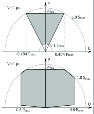
In the considered future scenarios, the time evolutions of wind speed and solar irradiance are assumed to be the same as in the 2013 recordings. Both wind turbines and PV units are categorized as non-dispatchable units since they are assumed to be internally controlled for MPPT. Two different capability diagrams are considered for reactive power support. The first one constrains the
unit to operate between power factors of 0.9 and 1.0 in both under- and over-excited modes, which leads to the triangle-shaped capability curve shown in the upper part on Figure 4. In the second diagram, operation is allowed inside the polygon-bounded surface shown in the lower part on Figure 4. This yields a larger reactive power reserve, the reactive power being limitedbetween 0.8Pmax when producing, and 0.6Pmax when consuming. At low or high active power production, the limits are restrained.
Figure 4 DGU capability diagrams. Operation is allowed in the shaded area
The future system is assumed to also host three CHP units. Since they are in operation for air-conditioning purposes mainly, their production schedule is pre-determined. Those units are categorized as dispatchable DGUs.
For all types of DGUs, as long as no violation is observed (or predicted), the reactive power is kept at zero with the objective of minimizing internal losses of the units. 4.3. Consumptions
The network feeds 420 residential and industrial loads connected to 297 MV buses.
The various residential loads connected at LV level and fed
by the same MV/LV transformer are aggregated into one load attached to the MV bus. That load also includes the losses in the LV network and in the MV/LV transformer. The industrial loads are subdivided into three types, depending on their consumption profile within a day:
• type 1: working during the day only (e.g. manufacturers; total number of 40);
• type 2: with high thermal needs (total number of 10); • type 3: working day and night (e.g. warehouses; total
number of 10).
There are also 178 heat pumps (total capacity of 1.37 MW) and 182 electrical vehicle charging stations (total capacity of 2.66 MW). Both are categorized as residential loads. 4.4. Measurements
With the expected penetration of DGUs, a better observability of the system will be needed, to detect and correct problems in various parts of the system. Hence, it is planned to install in a near future additional measurement points throughout the grid. The future telemetered values were assumed to be:
• the active and reactive powers injected by, and the terminal voltage of each DGU;
• the active and reactive power flows in all branches that leave the main substation;
• the active and reactive power flows in one incident branch and the voltage at each of the monitored buses shown with empty rectangles in Figure 3;
• the active and reactive powers received from the transformer(s) and the voltage(s) on their MV side. All those measurements are directly used by the MPC algorithm, as well as to update the reference active powers (13) and the reactive power limits (see Section 4.2). As suggested in Fig. 2, they could be pre-processed by a state estimator but that option is not considered here.
4.5. Selected scenarios
The simulations were run over full days, in order to assess the response of the controller to consumption/generation evolutions at different times of the day.
As already mentioned, historical data of wind speed, solar irradiance and load consumption have been exploited in this study. The data were available for the full year 2013, with a resolution of 15 min; linear interpolation has been used to obtain values at intermediate discrete times.
The following operation limits have been considered: voltages in the range [0.95, 1.05] pu at all buses, and the currents in cables and transformers below their thermal ratings.
The results reported here relate to three scenarios representative of stressed operating conditions:
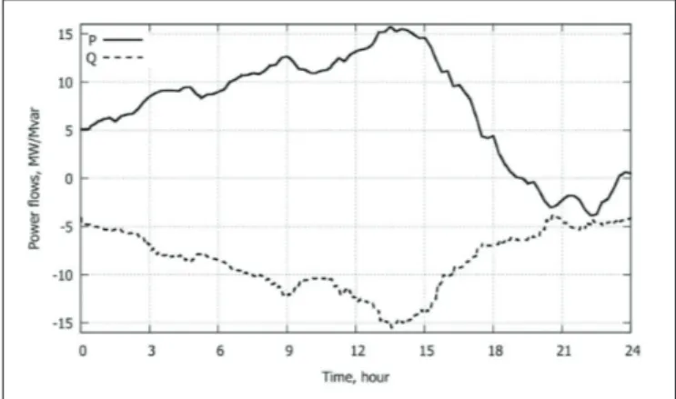
SD1: a summer day with high production by the DGUs. Combined with low load, this results in a high power transfer from distribution to transmission, as shown by the evolutions of the power flows in the transformer, see Figure 5 SD1, no controller: Active and reactive powers injected into the transmission system. CHP units are not in operation. The voltages at a sample of MV buses are given in Figure 6, showing that some voltages moderately exceed the upper limit. They increase as one moves from the main substation towards the end of a feeder; SD2: same scenario as SD1 but with a higher production
by wind generators. The corresponding same power flows are shown in Figure 7. The thermal limit of the transformer is exceeded between t ≈ 12 h and 15 h. The transformer tap position had been adjusted in order to avoid excessive voltages;
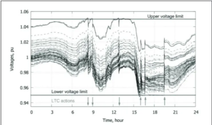
WD: a winter day with high power drawn from the transmission system. The wind speed is negligible and the PV units produce little power. Three CHP units come in operation during working hours. The corresponding power flows are shown in Figure 8. The two jumps in the active power flow are due to the rapid production changes of the CHP units. The voltage evolutions are given in Figure 9. One mild and one severe under-voltage situation are experienced. In addition, the transformer is overloaded between t ≈ 18 h and 22 h, but this situation is tolerable due to higher cooling capabilities in winter. It would be definitely safer to use the second transformer, but this option is not considered to demonstrate the effectiveness of the controller.
Figure 7 SD2, no controller: Active and reactive powers injected into the transmission system
Figure 6 SD1, no controller: Voltages at a sample of MV buses Figure 5 SD1, no controller: Active and reactive powers injected
To summarize, the three days involve different limit violations: over-voltage for SD1, thermal overload for SD2, under- and over-voltage for WD. The benefit of coordinating the DGU powers and the LTC voltage set-point will be illustrated in some variants.
4.6. Controller settings
The active power schedules of the CHP units are communicated every 15 minutes to the real-time controller, which is thus aware of those productions in advance. On the other hand, the wind and solar units are left to operate in MPPT mode (unless operating conditions do not allow doing so). No prediction of wind speed and solar irradiance is available to the controller.
The measurements are assumed to be received by the controller every 10 seconds, and its corrections sent to the DGUs and the LTC with the same periodicity.
In all simulations the sensitivity matrix Sl has been updated at each discrete step while the matrix has been kept constant at all times, to verify the robustness of the controller.
The control and prediction horizons have been set to Nc = Np = 3. Thus, the “open loop” control horizon is 3 × 10 = 30 seconds. In fact, the time taken by the controller to correct violations “in closed loop”, counted from its first action until a steady state is reached with all violations corrected, is in the order of 60 seconds. This holds true as long as no rate limit (9) is imposed, and the references Pref and Qref are left unchanged. This response time is fast enough for emergency control purposes. Note finally that it can vary with the number of active inequality constraints.
Within the guidelines stated in Section 2.2, there is quite some freedom in selecting the diagonal weighting matrices
R1, R2 and S. Their entries were merely set to: 1 for reactive powers, 25 for active powers, 500 for the slack variables ε1 and ε2, and 5000 for ε3. Unless otherwise specified, the voltage set-point of the LTC has been included in the control variables. To avoid excessive solicitation of that device (reducing its lifespan or requiring more frequent maintenance), its control has a lower priority (R3 = 10) compared to DGU reactive powers, with the result that it is used only when needed.
Simulations were performed with RAMSES, a dynamic simulation software developed at the University of Liège [27]. Each 10 min of real time is represented by 1 min of simulated time, for legibility of the results. The quadratic programming problem is solved using the Harwell procedure VE17AD [28].
4.7. Processing time
Each sampling period of the centralized controller can be decomposed into: (i) a communication delay for the control corrections to be received by the DGUs; (ii) a dead-time for the DGUs and their controllers to reach steady state after actuating those corrections; (iii) a time window in which the measurements are locally collected and pre-filtered; (iv) a communication delay for those measurements to be received by the controller; (v) the time taken by the MPC scheme to compute the corrections. As regards item (v), for the system of concern, the elapsed time to solve one optimization problem was found to vary between 0 and 32 ms, depending on the number of active constraints, which varies with time. Those times were obtained on a standard laptop computer with a dual-core Intel-i5 processor running at 2.27 GHz with 4 GB RAM.
Figure 9 WD, no controller: Voltages at a sample of MV buses Figure 8 WD, no controller: Active and reactive powers injected
In view of the number of measurements, it can be assumed that the delays (i) and (iv) together will not exceed 1 s. Considering a dead-time (ii) of 3 s, and a measurement window (iii) of 2 s, the five components sum up to 6 s, which leaves an ample margin with respect to the sampling period of 10 s.
5. Simulations results and
discussion
5.1. Case 1: SD1 with constant transmission voltage, triangle-shaped capability diagram
In this case, the voltage on the transmission side of the main transformer is assumed to remain constant, while the DGUs have the triangle-shaped capability diagram shown in the upper part of Figure 4.
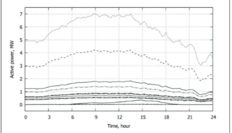
The evolutions of the active and reactive powers produced by DGUs are shown in Figure 10 Case 1: Active powers produced by DGUs and Figure 11 Case 1: Reactive powers produced by DGUs, respectively. The resulting voltage evolutions are shown in Figure 12.
For a little more than 15 hours, the DGUs are requested to consume reactive power in order to avoid over-voltages at the end of some feeders. It can be seen that after corrective control, the highest among all bus voltages is kept equal to (or smaller than) the maximum upper limit of 1.05 pu. The minimum consumption level is observed between midnight and sunrise. Therefore, from midnight up to T ≈ 4 h, the still decreasing consumption combined with some increase of the active generation causes a voltage rise. It is smoothly counteracted by reactive power adjustments of the DGUs to keep the voltages below the limit. Figure 11 Case 1: Reactive powers produced by DGUs1 shows the reactive power corrections of Eq. (12), in which the references Qref(k) have been specified to zero (see Section 4.2). It can be seen that the maximum correction takes place at T ≈ 4 h.
From this time till noon the production keeps on increasing, but its effects are counteracted by the consumption ramping in the morning. Since the system is controlled in such a way that limits are obeyed with minimum deviation of DGUs from unity power factor, one can observe a “reset” effect bringing the reactive powers towards zero. Thanks to centralized control, those DGUs closer to buses with higher voltage participate more in corrective control. Furthermore, the reactive power support of DGUs is significantly limited by the triangle-shaped capability diagram. In particular, this results in low reactive power reserves on units with low active power output.
During the last third of the day, production decreases while consumption increases. This leads to a decrease of voltages in the system. All voltages move away from
Figure 12 Case 1: Voltages of distribution buses
Figure 10 Case 1: Active powers produced by DGUs
the upper limit. Consequently, the DGU reactive powers come back to the desired zero value.
LTC control is not used since the reactive power changes are sufficient, and they are given priority through their weighting matrix in (2).
5.2. Case 2: SD1 with variable transmission voltage, triangle-shaped capability diagram
This case is identical to Case 1, except for the transmission voltage which varies together with the operating point of the distribution grid. To that purpose and for simplicity, the Thévenin equivalent voltage of the external grid linearly follows the active power injected by the distribution into the transmission grid. This aggravates the voltage violations in the MV network.
The bus voltages after corrective control are shown in Figure 13, while the DGU reactive powers are displayed in Figure 14. A comparison with Case 1 shows that more reactive power is consumed by the DGUs to keep voltages below the limit. The highest consumption is reached between T ≈ 12 h to T ≈ 15 h. Figure 15 shows that this coincides with the largest active power injection in the transmission grid and, consequently, the largest transmission voltage.
On the other hand, the peak demand in the evening causes an under-voltage which is corrected by the controller imposing a small production of reactive power.
Figure 14 Case 2 : Reactive powers produced by DGUs
Figure 15 Case 2: Active and reactive powers injected into the transmission system
5.3. Case 3: SD2 with constant transmission
voltage, polygon-bounded capability diagram, LTC non controlled
In this case, the transformer ratio is assumed constant, i.e. Vtap is removed from the control vector u in (1).
As mentioned previously, Scenario SD2 involves a violation of the transformer thermal limit, as shown by the dashed line in Figure 16, relative to the current in the transformer without corrective control.
At t ≈ 7 h the transformer current reaches its limit. This is detected by the centralized controller from the received measurements. The controller corrects this congestion by acting first on the DGU reactive powers, which have higher priority2.Figure 7 showed that the reactive power
Figure 13 Case 2: Voltages of distribution buses
2- The current in per unit is given by . Assuming that V does not change significantly (its value is anyway updated at each control step) and letting P unchanged, Q should be decreased to zero to decrease I
is flowing from the transmission to the distribution network. To alleviate the overload, that flow must be decreased, which requires to increase the DGU reactive power productions. The latter are shown in Figure 17. The solid line, which relates to a large number of DGUs with the same output, shows indeed an increase. However, an increase of all DGU reactive powers would cause over-voltages in the grid. This is why some other DGUs have their reactive power decreased, as shown by the dotted curves in Figure 17.
The reactive powers are exploited until the highest voltage reaches the allowed upper limit, as shown in Figure 18. At this point, the active powers of some DGUs must be decreased, until the remaining overload is cleared. Figure 19 shows the amount of curtailed active power of one DGU, imposed by the centralized controller.
A few hours later, a second thermal violation is detected and corrected in a similar but more pronounced manner. Figure 17 shows that two DGUs reached their maximum absorption capability.
At time t ≈ 16 h, the power consumption of loads increases, while the wind speed decreases. This allows the powers of the wind units to progressively reach their maximum available values, as confirmed by Figure 19 showing that the correction sent by the controller decreases to zero.
Figure 16 Case 3: Current in the transformer
Figure 18 Case 3: Voltages of distribution buses Figure 17 Case 3: Reactive powers produced by the DGUs
Figure 22 Case 4: Voltages of distribution buses) and by reducing the DGU reactive powers. Incidentally, this voltage adjustment explains the slightly different values of the current, with and without control (dashed vs. solid line in Figure 20), while the transformer is not overloaded any more.
Figure 20 Case 4: Current in the transformer
Figure 21 Case 4: Reactive powers produced by the DGUs
Figure 22 Case 4: Voltages of distribution buses 5.4. Case 4: SD2 with constant transmission
voltage, polygon-bounded capability diagram This case is similar to the previous one, except that the centralized controller again can adjust the voltage set-point Vtap of the transformer LTC. The latter can be used to mitigate the over-voltages caused by DGU reactive powers, as shown hereafter.
The successful correction of the transformer overload is seen in Figure 20.
As in Case 3, to reduce the current in the transformer, the reactive power flowing from transmission to distribution must be decreased, which requires to increase the DGU reactive powers. This is shown in Figure 21.
The evolution of the distribution voltages is given in Figure 22 . They are all kept within the allowed limits. As in Case 3, the reactive power injected by the DGUs between t ≈ 7 h and t ≈ 16 h would lead to over-voltages but the controller prevents this by decreasing the LTC voltage set-point Vtap. This takes place at three times, identified with down arrows inFigure 22. The effects are visible in all voltage evolutions. With this contribution by the LTC, there is no need for some DGUs to consume reactive power as in Case 3 (see Figure 17). On the contrary 21 shows that more DGUs contribute with reactive power production.
The main benefit of the LTC actions is the smaller amount of active power curtailment in complement to the reactive power corrections. This is illustrated in Figure 23, to be compared with Figure 19 of Case 3. Further evidence is given inFigure 24, which compares the active power flows in the transformer in Cases 3 and 4, respectively. The additional LTC control allows exporting to the transmission system 0.4 MW more, on the average, between t ≈ 12 h and t ≈ 15 h.
From t ≈ 16 h to t ≈ 19 h, the system is exposed to under-voltages (caused by evening load increase and DGU power decrease). This voltage drop was already seen in Figure 18 of Case 3, but is more severe here due to the previous LTC interventions. The controller keeps the voltages above the lower limit by changing Vtap in the opposite direction (as shown by the up arrows in
Figure 25 Case 5: Voltages of distribution buses
Figure 26 Case 5: Reactive powers produced by the DGUs 5.6. Case 6: WD with variable transmission voltage, triangle-shaped capability diagram
Finally, Case 5 is revisited, assuming that DGUs have tighter reactive power limits: the polygon-bounded capability diagram is replaced by the triangle-shape one (see Figure 4). The controller compensates for the lack of reactive power reserves by resorting to 16 tap changes over the whole day (instead of five in Case 5). This allows keeping all voltages between limits, as shown by Figure 27. A comparison with Figure 25 shows that the voltage violations last longer when they are corrected by the LTC mainly. This is due to the (unchanged) LTC internal delays: s on the first tap change, s between subsequent tap changes.
Figure 28 reveals very small DGU reactive power variations before t ≈ 7 h and after t ≈ 19 h. At those times, the DGU active power productions are close to zero and, hence, the triangle-shaped capability diagram does not allow significant reactive power variations.
Figure 23 Case 4: Active power curtailment applied to DGU 2032
Figure 24 Active power injected into the transmission system: Case 3 vs. Case 5.5. Case 5: WD with variable transmission
voltage, polygon-bounded capability diagram In this case the controller acts to correct the unacceptable voltages observed in Figure 9. The corrected voltage evolutions are shown in Figure 25. Over-voltages are avoided at t ≈ 13 h and t ≈ 23 h, when consumption is relatively low, while under-voltages are corrected at t ≈ 7 h and t ≈ 19 h, which corresponds to morning ramp and evening peak, respectively. The corresponding adjustments of the DGU reactive powers are shown in Figure 26. Although LTC control has lower priority compared to DGU reactive powers, it must be used to raise the very low evening voltages. The corrections result in five transformer tap changes, identified in Figure 25.
As for any centralized control, the main burden of the proposed scheme is to collect all measurements in, and send all controls from a single place. This requires a communication infrastructure. It is, however, the trend in modern distribution management systems to have a “system-wide” view of the system as advocated in this paper.
Compared to the traditional OPF approach, the proposed scheme :
• offers robustness against modeling inaccuracies, measurement errors, control actuation failure, and loss of communication
• “steers” the system from the current (non-viable) to the desired (safe) operating state. It does so smoothly, avoiding large transients that could stress equipment. The simulations reported in this paper involved future scenarios of a real-life distribution system. The paper has demonstrated the controller performance over three full days, identified as challenging in terms of voltage and/or thermal violations. The following features were stressed:
• priority given to “cheap” control actions
• active power curtailment minimized as much as possible,
• DGUs powers brought back at their desired values once corrections are no longer needed
• repeated optimization compatible with the efficiency constraints of a real-time controller.
On the premise that operation limits are exceeded for limited durations, the above demonstrated features make the proposed corrective control scheme a serious alternative to expensive network reinforcements, and contribute to removing one obstacle to the penetration of renewable energy sources in modern distribution grids. The approach can be directly applied to devices such as D-STATCOMs. On the other hand, further investigations are considered for the control of:
• shunt capacitors, their susceptance being treated as a discrete variable
• flexible loads, which requires incorporating energy consumption constraints over longer periods than the short-term considered in this paper
• battery storage, taking into account their state of charge and other specific constraints
In between t ≈ 7 h and t ≈ 19 h, CHP and PV units are producing active power and, hence, can contribute with larger reactive power adjustments.
Figure 27 Case 6: Voltages of distribution buses
Figure 28 Case 6: Reactive powers produced by the DGUs
6. Conclusion
A centralized corrective control of voltages and/or thermal violations in distribution networks has been presented. Based on the principle of MPC, the controller involves a multi-step constrained optimization. The scheme can be applied to two types of DGUs: dispatchable and non-dispatchable. The objective is to capture maximum power available from renewable DGUs or deviate as few as possible from pre-defined schedules, while keeping the grid within operation limits. Thus, the controller does not act as long as the system operates within the specified limits. With its “wide view” of the system (through the sensitivity matrices), the controller adjusts the DGU powers and the voltage set-point of the LTC in a coordinated manner; this performance could not be obtained with simple distributed control, and will become more important as distribution grids will host more and more DGUs.
[12] R. Godina, E.M.G. Rodrigues, J.C.O. Matias, and J.P.S. Catalão, “Smart Electric Vehicle Charging Scheduler for Overloading Prevention of an Industry Client Power Distribution Transformer,” Applied Energy, 178:29–42, sep 2016.
[13] I. Abdelmotteleb and J.P. Chaves-Avila, “Benefits of PV Inverter Volt-Var Control on Distribution Network Operation,” In Proc. IEEE PowerTech Conference, Manchester (UK), 2017.
[14] K. Das, E. Nuno Martinez, M. Altin, A. Daniela Hansen, and G. Wad Thybo, “Facing the Challenges of Distribution Systems Operation with High Wind Power Penetration,” In Proc. IEEE PowerTech Conference, Manchester (UK), 2017.
[15] P. Kotsampopoulos, N. Hatziargyriou, B. Bletterie, and G. Lauss, “Review, Analysis and Recommendations on Recent Guidelines for the Provision of Ancillary Services by Distributed Generation,” In Proc. IEEE International Workshop on Inteligent Energy Systems (IWIES), pages 185–190, Vienna (Austria), nov 2013.
[16] T. Sansawatt, L.F. Ochoa, and G.P. Harrison, “Smart Decentralized Control of DG for Voltage and Thermal Constraint Management,” IEEE Transactions on Power Systems, 27(3):1637–1645, aug 2012. [17] S. Asadollah, R. Zhu, M. Liserre, and C. Vournas, “Decentralized
Reactive Power and Voltage Control of Wind Farms with Type-4 Generators,” In Proc. IEEE PowerTech Conference, Manchester (UK), 2017.
[18] B.A. Robbins, C.N. Hadjicostis, and A.D. Dominguez-Garcia, “A Two-Stage Distributed Architecture for Voltage Control in Power Distribution Systems,” IEEE Transactions on Power Systems, 28:1470–1482, may 2013.
[19] J. Hambrick and R.P. Broadwater, “Configurable, Hierarchical, Model-Based Control of Electrical Distribution Circuits,” IEEE Transactions on Power Systems, 26(3):1072–1079, aug 2011. [20] H. Soleimani Bidgoli and T. Van Cutsem, “Combined Local and
Centralized Voltage Control in Active Distribution Networks,” IEEE Transactions on Power Systems, 33(2): 1374-1384, mar 2018.
[21] J. M. Maciejowski, “Predictive Control with Constraints,” Prentice-Hall, Essex (UK), 2002.
[22] S.J. Qin and T.A. Badgwell, “A Survey of Industrial Model Predictive Control Technology,” Control Engineering Practice, 11(7):733–764, jul 2003.
[23] A. Bemporad and M. Morari, “Robust model predictive control: A survey,” In Robustness in identification and control, pages 207– 226. Springer, London (UK), 1999.
[24] G. Valverde and J.J. Orozco, “Reactive Power Limits in Distributed Generators from Generic Capability Curves,” In Proc. IEEE PES General Meeting, Washington DC (USA), jul 2014.
[25] G. Valverde and T. Van Cutsem, “Control of Dispersed Generation to Regulate Distribution and Support Transmission Voltages,” In Proc. IEEE Grenoble Conference, Grenoble (France), jun 2013. [26] B. Cornélusse, D. Vangulick, M. Glavic, and D. Ernst, “Global
Capacity Announcement of Electrical Distribution Systems: A Pragmatic Approach,” Sustainable Energy, Grids and Networks, 4:43–53, dec 2015.
[27] P. Aristidou, D. Fabozzi, and T. Van Cutsem, “Dynamic Simulation of Large-Scale Power Systems Using a Parallel Schur-Complement-Based Decomposition Method,” IEEE Transactions on Parallel and Distributed Systems, 25(10):2561–2570, oct 2014.
but also for practical issues such as:
• the control transitions after a change of topology of the distribution grid
• the incorporation of DGU dynamics in the state prediction, e.g. for slowly responding units.
7. Acknowledgment
This research was supported by Public Service of Wallonia, Department of Energy and Sustainable Building within the GREDOR project.
8. References
[1] S. Chowdhury, S. P. Chowdhury, and P. Crossley, “Microgrids and Active Distribution Networks,” The Institution of Engineering and Technology (IET), London (UK), 2009.
[2] J.A. Peças Lopes, N. Hatziargyriou, J. Mutale, P. Djapic, and N. Jenkins, “Integrating Distributed Generation into Electric Power Systems: A Review of Drivers, Challenges and Opportunities,” Electric Power Systems Research, 77(9):1189–1203, jul 2007. [3] Q. Gemine, E. Karangelos, D. Ernst, and B. Cornélusse, “Active
Network Management: Planning Under Uncertainty for Exploiting Load Modulation,” In Proc. IREP Symposium on Bulk Power System Dynamics and Control, Rethymnon (Greece), aug 2013. [4] V.A. Evangelopoulos, P.S. Georgilakis, and N.D. Hatziargyriou,
“Optimal Operation of Smart Distribution Networks: A Review of Models, Methods and Future Research,” Electric Power Systems Research, 140:95–106, nov 2016.
[5] H. Soleimani Bidgoli, M. Glavic, and T. Van Cutsem, “Model Predictive Control of Congestion and Voltage Problems in Active Distribution Networks,” In Proc. CIRED Workshop, number 0108, Rome (Italy), jun 2014.
[6] H. Soleimani Bidgoli, M. Glavic, and T. Van Cutsem, “Receding-horizon Control of Distributed Generation to Correct Voltage or Thermal Violations and Track Desired Schedules,” In Proc. 19th Power System Computation Conference (PSCC), Genova (Italy), jun 2016.
[7] G. Valverde and T. Van Cutsem, “Model Predictive Control of Voltages in Active Distribution Networks,” IEEE Transactions on Smart Grid, 4(4):2152–2161, dec 2013.
[8] P.N. Vovos, A. E. Kiprakis, A. R. Wallace, and G. P. Harrison, “Centralized and Distributed Voltage Control: Impact on Distributed Generation Penetration,” IEEE Transactions on Power Systems, 22(1):476–483, feb 2007.
[9] M. Farina, A. Guagliardi, F. Mariani, C. Sandroni, and R. Scattolini, “Model Predictive Control of Voltage Profiles in MV Networks with Distributed Generation,” Control Engineering Practice, 34:18–29, jan 2015.
[10] M.J. Dolan, E.M. Davidson, I. Kockar, G.W. Ault, and S.D.J. McArthur, “Distribution Power Flow Management Utilizing an Online Optimal Power Flow Technique,” IEEE Transactions on Power Systems, 27(2):790–799, may 2012.
[11] H. Soleimani Bidgoli, “Real-time Corrective Control in Active Distribution Networks”, Ph.D. thesis, Univ. of Liège, Dec. 2017, available: https://orbi.uliege.be/handle/2268/218339?locale=en
affiliations include: the University of Wisconsin- Madison (USA) as a Fulbright postdoctoral scholar, the University of Liege (Belgium) as senior research fellow and visiting professor, and Quanta Technology (USA) as senior advisor. He is presently a senior research fellow at the University of Liege. His research interests are in power system dynamics, stability, optimization, and real-time control.
Thierry Van Cutsem graduated in Electrical-Mechanical Engineering from the University of Liège, Belgium, where he obtained the Ph.D. degree and he is now adjunct professor. Since 1980, he has been with the Fund for Scientific Research (FNRS), of which he is now a Research Director. His research interests are in power system dynamics, stability, security, monitoring, control and simulation. He has been active in several CIGRE Working Groups. He also served as Chair of the IEEE PES Power System Dynamic Performance Committee. He is a Fellow of the IEEE.
[28] HSL, “A Collection of Fortran Codes for Large Scale Scientific Computation,” Available: http://www.hsl.rl.ac.uk, 2011.
9. Biographies
Hamid Soleimani Bidgoli received his B.Sc. degree in Electrical Engineering from IUST, Tehran, Iran and his M.Sc. in the same field from university of Tehran, Tehran, Iran, in 2008 and 2010, respectively. During 2010 to 2013, Hamid worked in Energy sectors in MAPNA group, Tehran, Iran. Then, getting back to academia, he obtained his Ph.D. in Electrical Engineering from the University of Liège, Belgium in 2017. He is currently an Electrical specialist at CMI Energy Storage, Belgium. His main scientific interests are active network management of distribution networks, real-time control, energy storage system, and demand side management.
Mevludin Glavic received the M.Sc. and Ph.D. degrees from the University of Belgrade (Serbia) and Tuzla (Bosnia) in 1991 and 1997, respectively. His previous