3D-model view characterization using equilibrium planes

HAL Id: hal-00668004

https://hal.archives-ouvertes.fr/hal-00668004

Submitted on 8 Feb 2012

HAL is a multi-disciplinary open access

archive for the deposit and dissemination of

sci-entific research documents, whether they are

pub-lished or not. The documents may come from

teaching and research institutions in France or

abroad, or from public or private research centers.

L’archive ouverte pluridisciplinaire HAL, est

destinée au dépôt et à la diffusion de documents

scientifiques de niveau recherche, publiés ou non,

émanant des établissements d’enseignement et de

recherche français ou étrangers, des laboratoires

publics ou privés.

3D-model view characterization using equilibrium planes

Adrien Theetten, Tarik Filali Ansary, Jean-Philippe Vandeborre

To cite this version:

Adrien Theetten, Tarik Filali Ansary, Jean-Philippe Vandeborre. 3D-model view characterization

using equilibrium planes. 4th International Symposium on 3D Data Processing, Visualization and

Transmission (3DPVT’08), Jun 2008, Atlanta, Georgia, United States. pp.117. �hal-00668004�

3D-Model view characterization using equilibrium planes

Adrien Theetten

_{, Tarik Filali Ansary}

_{, Jean-Philippe Vandeborre}

1

_{LIFL (UMR CNRS-USTL 8022), University of Lille 1, France}

2

_{Institut TELECOM; TELECOM Lille 1, France}

main contact: jean-philippe.vandeborre@lifl.fr

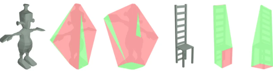
Figure 1. Two database objects and their respective convex hull. Green faces correspond to equilib-rium planes and thus to characteristic views.

Abstract

We propose a new method for 3D-mesh model charac-teristic view selection. It consists in using the views that come from the equilibrium states of a 3D-model: they cor-respond to the horizontal plane on which an object is stat-ically laying under the effect of gravity. The selected views are then very intuitive for the user. Indeed, to present a query, the user will take a photo or draw a sketch of the object on a table or on a floor, putting thus the object in a static mechanical equilibrium. Consequently, our view se-lection method follows the same principles: finding all the equilibrium planes of an object and obtaining their relative 2D views. We present the experiments and results of our method on the Princeton 3D Shape Benchmark Database using a collection of 50 images (photos, sketches, etc.) as queries, showing the performance of our method in 3D re-trieval from photos.

1

Introduction

The human visual system has an uncanny ability to rec-ognize objects from single views, even when presented monocularly under a fixed viewing condition. For exam-ple the identity of most of the 3D-models in figure 5 – in the rest of the paper, the term model” refers to

“3D-mesh model” – is immediately clear. The issue of whether 3D-model recognition should rely on internal representa-tions that are inherently three-dimensional or on collecrepresenta-tions of two-dimensional views, has been explored by Risenhu-ber and Poggio [18]. They show that, in a human vision system, a 3D-model is represented by a set of 2D views. The main idea of view-based similarity methods is that two 3D-models are similar, if they look similar from all viewing angles. This paradigm leads to the implementation of query interfaces based on defining a query by one or more views, sketches, photos, from different points of views. To search a database for 3D-models that are visually similar, using a view, a sketch or a photo of a 3D-model is a very intuitive way. However the main question is how to select canonical, natural, 2D views to represent and characterize a 3D-model. Blanz et al. [2] as well as Cutzu and Edelman [7] showed that, the source of canonicality are stability, familiarity and functionality. For example, Cyr and Kimia [8] use an as-pect graph to represent a 3D-model. The number of views is kept small by clustering views and by representing each cluster by one view, which is described by a shock graph. Chen et al. [4] use 100 orthogonal projections of an ob-ject and encode them by Zernike moments and Fourier de-scriptors. The running time of the retrieval process is re-duced by a multi-step approach supporting early rejection of non-relevant models. Nayar et al. [16] consider each 3D-model as a cloud of points. Principal axes of each 3D

model are calculated using the eigenvalues of the matrix of covariance. The 3D-model cloud of points are projected into 2D according to the three principal directions thus cal-culated. Seven characteristic views are created, three princi-pal views along the principrinci-pal axes and four views according to four directions corresponding of 45◦ views between the principal views. Yamauchi et al. [20] use a uniform sam-pling of viewpoints along the surface of a bounding sphere. Stable view regions are computed by a graph partition al-gorithm where the edges are weighted by view similarity, using Zernike moment analysis. However, the computation time of the graph is about 40 minutes per model. Then 8 characteristic views are obtained by ranking the regions with view saliency. Filali et al. [10] propose an algo-rithm, called Adaptive View Clustering (AVC) to choose the characteristic views of a 3D-model. Their method relates the number of views to its geometrical complexity. Start-ing from 320 viewpoints, equally spaced on the boundStart-ing sphere, the algorithm selects the optimal views, clustering them with Zernike moment descriptor [14]. The resulting number of views varies from 1 to 40, depending on the ob-ject complexity. The view selection takes about 18 seconds per model.

In this paper, we propose a new method for 3D-model characteristic view selection. It is not based on human per-ception elements, but on a physical process that consists in considering only the views that come from the static equi-librium states of a 3D-model. However, these views are very familiar and intuitive for the user: they correspond to the horizontal plane on which an object is statically laid un-der the effect of gravity. Indeed, to present a query, the user will take a photo or draw a sketch of the object on a table or on a floor, putting thus the object in a static mechanical equilibrium. Consequently, our view selection method fol-lows the same principles: finding all the equilibrium states – i.e. all the equilibrium planes – of an object and obtaining their relative 2D view. Then finally, these 2D-views are fil-tered to delete the similar views modulo a translation and/or a rotation.

This paper is organized as follows. The next section is dedicated to the computation of the equilibrium planes of a 3D-model. Then, the third section presents the charac-teristic view determination according to the corresponding computed orientations. Finally, we present the experiments and results of our method on a database composed of 1814 3D-models (Princeton 3D Shape Benchmark Database) us-ing a collection of 50 images (photos, sketches, etc.) as queries, showing the performance of our method in 3D re-trieval from photos.

2

Equilibrium plane computation

In order to estimate the characteristic views of a 3D-model, we consider equilibrium planes. An equilibrium plane of an object – i.e. a plane on which the object is laid under gravity – is defined by its normal direction n. It is a natural and intuitive object orientation that we can reproduce easily, independently from its dimensions or its weight. The corresponding characteristic view to an equi-librium plane is entirely determined by the direction of its plane.

In this section, we first elucidate some terminology on equilibrium planes. Then, we propose a simple and efficient method to compute the equilibrium planes of a 3D-model. We finally describe how to get the corresponding character-istic views.

2.1

Equilibrium plane terminology

An equilibrium plane of an object – i.e. a plane on which the object is laying under gravity – is defined by the normal plane direction n. In order to find the equilibrium planes of a 3D-model, the convex-hull and the center of mass of the 3D-model first need to be computed.

2.1.1 Convex-hull construction

The convex hull of a 3D-model is the smallest convex poly-hedron containing the model point cloud. It is a funda-mental construction for mathematics and computational ge-ometry. Many problems use or can be reduced to con-vex hulls: mesh generation, file searching, collision detec-tion, cartography, etc. Its construction can be achieved in many ways [17]. Some methods use deterministic incre-mental algorithms [9] or randomized increincre-mental construc-tion [5, 1]. In our approach, we choose the CGAL imple-mentation of the QuickHull algorithm [1]. It handles all degenerate cases and non-manifold models that constitute our 3D-model database. In the worst case this algorithm is O(n2), but in practice it is no worse than O(n log(n)), where n is the number of vertices of a 3D-model.

2.1.2 Center of mass and volume computation

The calculation of the center of mass and the volume of rigid bodies has been extensively treated in literature. Mir-tich [15] proposes an efficient method to compute the center of mass for polyhedral objects. Its algorithm is based upon a three-step reduction of the volume integrals to successively simpler integrals. The final step of the algorithm computes the required integrals over a face from the coordinates of the projected vertices. Considering that mass distribution is ho-mogeneous in the 3D-model volume V , the center of mass G thus yields:

G = 1 V Z V   x y z   dV (1)

Gonzalez et al. [12] exploit the divergence theorem, that transforms an integral over a volume into an integral over its boundary surface. An orthogonal projection along the z direction thus results in a more convenient and efficient integral, as follows: G = 1 V Z S sign(nz)   x y z/2  zdxdy (2)

where S is the surface boundary of the 3D-model, n is the normal at point P (x, y, z) and sign(x) denotes the signum function which extracts the sign of a real number x. Using the divergence theorem, the 3D-model volume V yields:

V = Z

S

sign(nz)zdxdy (3)

The overall complexity of the two integrals is O(m), where m represents the number of faces of the polyhedron. A very efficient method using GPU shaders is proposed by Kim et al. [13].

The convex hull and center of mass constitute a main part of the equilibrium plane computation we propose in the next subsection.

2.2

Equilibrium plane computation

We use the following necessary and sufficient conditions to compute an equilibrium plane:

Theorem 1 A direction n defines an equilibrium plane E if and only if there exists a plane π of normal n such that it contains a faceFi of the convex hullH of the 3D-model

(convex hull condition)and if the projection of the center of massG of the 3D-model along n is inside Fi(center of

mass condition).

Proof A static mechanical equilibrium requires that at least three non collinear points of the 3D-model belong to π. Since π is not a separating plane of the 3D-model points, it necessarily contains a face Fiof the convex hull H.

Let us suppose the projection of G along n onto π does not belong to Fi. The gravity force applied on G thus exerts

a moment whose axis ∆ is the nearest edge of Fi from G.

The ground force also exerts a moment on ∆, that does not oppose to the gravity moment. So their resultant moment on ∆ is not zero and the 3D-model is thus not in static equi-librium (see figure 2). The projection of G along n onto π must consequently belong to Fi.

Figure 2. Two configurations verifying the convex hull condition and eligible to be an equilibrium plane; however the left one does not verify the center of mass condition and leads to the right one.

Algorithm 1 provides the equilibrium plane computa-tion. Figure 1 illustrates the result for two database objects. Robustness and time complexity of our algorithm are domi-nated by the convex hull construction (nlog(n) for a n point model).

Algorithm 1 Equilibrium plane algorithm Compute the visual hull H.

Compute the center of mass G. for all faces Fiof H do

Project orthogonally G on plane π containing Fi:

P (G).

if P (G) ∈ Fithen

Add π direction n to the equilibrium plane list. end if

end for

3

Characteristic view determination

Figure 3 presents the corresponding physical-based views to the seven equilibrium planes of a humanoid 3D-model.

The views extracted from the equilibrium planes are sil-houettes only, which enhance the efficiency and the robust-ness of the image metric. The view direction has been ar-bitrarily fixed to the othogonal direction according to the equilibrium plane. To represent each of these 2D views, we use 30 coefficients of the Zernike moment descriptor [14]. Due to the use of Zernike moments, our image metric is invariant to translation, rotation, and scaling.

The extraction of the Zernike moments of characteristic views and query images is as follows:

1. Transform input image to grey scale image.

2. Get edge image from the grey level image using the Canny filter[3] and binarize it, the object is composed of the edge pixels.

3. Normalise the binarized edge image to accomplish ob-ject scale invariance.

4. Move the origin of the image to the centroid of the object, obtain object translation invariance.

5. Extract up to the ninth order Zernike moments corre-sponding to 30 features.

As the reader may have noticed, in figure 3 the views v0, v2, v4 and v5 are similar, as well as the views v1 and v6. This primary set of views has to be reduced to the only ones that best characterize this 3D-model. In order to delete the similar views modulo a translation and/or a rotation trans-formation, a Nearest Neighbor clustering [6] is used. To compare two views, we use the Euclidean distance between their corresponding Zernike moments. After several experi-ments, we used a distance threshold ε = 0.07 that gives the best performances.

Figure 3. Seven equilibrium planes for this humanoid 3D-model give seven primary views (v0 to v6).

Figure 4 (a) shows the result of the Nearest Neighbor clustering applied to the views of figure 3. The three charac-teristic views of figure 4 represent the humanoid 3D-model. Figure 4 (b) shows the characteristic views representing a chair 3D-model.

4

Experiments and results

In this section, we present the experimental process and the results we obtained. The algorithms we described in the previous sections have been implemented using C++, CGAL library and Java 3D. The system consists of an of-fline view extraction algorithm and an online retrieval pro-cess.

In the offline process – the equilibrium plane computa-tion – the view extraccomputa-tion and the filtering steps take about 43 seconds per 3D-model on a 3GHz Pentium IV PC. In the online process, the comparison with the 1814 3D-models requires less than 1 second.

To evaluate our method, we used the Princeton Shape Benchmark database [19], a standard shape benchmark

(a) Humanoid 3D-model

(b) Chair 3D-model

Figure 4. (a) Three final views (v0, v1 and v3) after the filtering of the seven primary views of the humanoid 3D-model (figure 3). (b) Three final views representing the chair 3D-model.

widely used in the shape retrieval community. The Prince-ton Shape Benchmarkappeared in 2004 and is one of the most exhaustive benchmarks for 3D shape retrieval. It con-sists in a collection of 1814 classified 3D-models collected from 293 different Web domains. There are many classi-fications given to the objects in the database. During our experiments, we used the finest granularity classification, composed of 161 classes. Most classes contain objects with a particular function (e.g cars). Yet, there are also cases where objects with the same function are partitioned in dif-ferent classes based on their shapes (e.g, round tables versus rectangular tables).

Using our method, the mean number of views for the Princeton Shape Benchmark databaseis 4 views per model. The mean size for a 3D-model descriptor is 240 bytes.

To evaluate the retrieval algorithms, we presented in the previous sections, we used the images from the photos col-lection proposed by Filali et al. [11]. This colcol-lection con-tains images corresponding to 10 classes of the Princeton Shape Benchmark (five images per class): Airplanes, Bi-cycles, Chairs, Dogs, Guns, Hammers, Humans arms out, Helicopters, Pots and Swords (figure 5 shows image exam-ples). The images are composed of six sketches, six synthe-sized images and thirty-eight real photos of different size. As the reader may have noticed, we use query-images with a simple background. This problem can be partially solved using a more sophisticated segmentation algorithm, but this is beyond the scope of this paper. It is also important to note that the query-photos are not necessarily obtained from equilibrium states.

To objectively evaluate our method, we used the Near-est Neighbor, First Tier and Second Tier statistical crite-ria, as well as Recall vs. Precision and Cumulative

re-(a) bicycles (b) chairs

(c) airplanes (d) humans (e) pots

Figure 5. Some images used as queries.

call curve. These are well-known criteria used in the multimedia-retrieval litterature and are explained below.

• Nearest neighbor: the percentage of the closest matches that belong to the same class as the query. This statistic provides an indication of how well a near-est neighbor classifier would perform. Obviously, an ideal score is 100%, higher scores represent better re-sults.

• First-Tier and Second-Tier: the percentage of mod-els in the query’s class that appear within the top K matches, where K depends on the size of the query’s class. Specifically, for a class C with |C| members, K = |C| − 1 for the first tier, and K = 2 × (|C| − 1) for the second tier. In all cases, an ideal matching re-sult gives a score of 100%, again higher values indicate better matches.

Table 1 shows the storage requirements in bytes (we used four views which is the average number of characteristic views for all the database models) and retrieval statistics for our algorithm on the Princeton Shape Benchmark database. Due to the use of photos and sketches as queries, results cannot be compared with those obtained with 2D projec-tions of the 3D-model in the database [10].

Storage size Nearest Neighbor 1st Tier 2nd Tier 240 32.4% 18% 23%

Table 1. Retrieval performances for the Princeton 3D Shape Benchmark database.

Figure 6(a) presents the cumulative recall curve for five of the ten used classes. This curve represents the evolu-tion of the recall score in the first 100 results. From this curve we can notice the good retrieval performances of our method using only one photo as a query. Figure 6(b) shows the Recall Vs Precision plots for the five image-classes pre-sented in figure 5. We can notice that our method gives good retrieval results using one image. Figure 7, shows that our approach gives comparable retrieval results with the Adap-tive Views Clustering method [11] on bikes, chairs and

pot-(a) Cumulative recall curve

(b) Recall Vs. Precision curve

Figure 6. The cumulative recall and the recall precision curves for the first 100 results on the Princeton Shape Benchmark database.

ted plants classes using six times less space and five times quicker.

On the one hand, the airplane class Recall vs Precision plot (Figure 7(d)) shows the limits of our method. The bad retrieval results are due to the fact that the majority of pho-tos of airplanes in this image database are not taken from equilibrium state views. On the other hand, the good results of the bike class prove the huge potential of our method with queries only composed of equilibrium state views. Indeed, bike photos are always laterally taken and thus correspond to such views.

5

Conclusion

In this paper, we propose a new method for 3D-model characteristic view selection. It introduces a new physically based criterion for the view selection. Characteristic views correspond to the planes on which the object is laid under gravity (equilibrium planes). We first propose a simple and efficient method to compute the equilibrium planes of a 3D-model. Then using a nearest neighbor clustering on these 2D-views, the similar views are filtered modulo a transla-tion or a rotatransla-tion. The average number of views to represent

(a) Potted plants (b) Chairs

(c) Bikes (d) Airplanes

Figure 7. Recall Precision on the Prince-ton Shape Benchmark database for the AVC method [10] and ours, with one image queries.

a 3D-model is 4 and the average 3D-model descriptor is 240 bytes only.

Based on some standard measures, we present the ex-periments and results of our method on a database com-posed of 1814 3D-models (Princeton 3D Shape Benchmark Database) using a collection of 50 images (photos, sketches, etc.) as queries, showing the performance of our method in 3D retrieval from photos.

Our approach gives a good quality/cost compromise compared to the AVC method [10]. Moreover, a promis-ing retrieval protocol could be designed, uspromis-ing only queries corresponding to equilibrium plane views and using more than one photo as a query. In future works, we propose to establish such a protocol and also plan to improve the equilibrium computation by considering non homogeneous weight 3D-models.

Acknowledgments

This work has been partially supported by the ANR (Agence Nationale de la Recherche, France) through MADRAS project (ANR-07-MDCO-015).

References

[1] C. B. Barber, D. Dobkin, and H. Huhdanpaa. The quickhull algorithm for convex hulls. ACM Transactions on Mathe-matical Software, 22(4):469–483, 1996.

[2] V. Blanz, T. Vetter, H. Bulthoff, and M. Tarr. What object attributes determine canonical views. Perception, 24(Sup-plement), 119c., 1995.

[3] J. F. Canny. A computational approach to edge detection. IEEE Transactions on Pattern Analysis and Machine Intelli-gence, 8(6):679–698, 1986.

[4] D. Y. Chen, X. P. Tian, Y. T. Shen, and M. Ouhyoung. On visual similarity based 3D model retrieval. In Eurographics, volume 22, pages 223–232, 2003.

[5] K. L. Clarkson, K. Mehlhorn, and R. Seidel. Four results on randomized incremental constructions. Computational Geometry: Theory and Applications, pages 185–121, 1993. [6] T. Cover and P. Hart. Nearest neighbor pattern classification.

IEEE Transactions on Information Theory, 13:21–27, 1967. [7] F. Cutzu and S. Edelman. Canonical views in object repre-sentation and recognition. Vision Research, 34:3037–3056, 1994.

[8] C. M. Cyr and B. Kimia. 3D object recognition using shape similarity-based aspect graph. In IEEE International Con-ference on Computer Vision, pages 254–261, 2001. [9] I. Z. Emiris. A complete implementation for computing

general dimensional convex hulls. International Journal of Computational Geometry and Applications, 8(2):223+, 1998.

[10] T. Filali Ansary, M. Daoudi, and J.-P. Vandeborre. A bayesian 3D search engine using adaptive views cluster-ing. IEEE Transactions on Multimedia, 9(1):78–88, January 2007.

[11] T. Filali Ansary, J.-P. Vandeborre, and M. Daoudi. On 3D retrieval from photos. In 3rd IEEE International Sym-posium on 3D Data Processing Visualization Transmission (3DPVT), 2006.

[12] C. Gonzalez-Ochoa, S. McCammon, and J. Peters. Comput-ing moments of objects enclosed by piecewise polynomial surfaces. ACM Transactions on Graphics, 17(3):143–157, 1998.

[13] J. Kim, S. Kim, H. Ko, and D. Terzopoulos. Fast GPU com-putation of the mass properties of a general shape and its application to buoyancy simulation. The Visual Computer, 22(9):856–864, 2006.

[14] W.-Y. Kim and Y.-S. Kim. A region-based shape descriptor using Zernike moments. Signal Processing: Image Commu-nication, 16(1-2):95–102, 2000.

[15] B. Mirtich. Fast and accurate computation of polyhedral mass properties. Journal of graphics tools, 1(2):31–50, 1996.

[16] S. Nayar, S. A. Nene, and H. Murase. Real–time ob-ject recognition system. In International Conference on Robotics and Automation, 1996.

[17] F. P. Preparata and S. J. Hong. Convex hulls of finite sets of points in two and three dimensions. Commun. ACM, 20(2):87–93, 1977.

[18] M. Riesenhuber and T. Poggio. Computational models of object recognition in cortex: A review. Technical report, Artificial Intelligence Laboratory, MIT, 2000.

[19] P. Shilane, P. Min, M. Kazhdan, and T. Funkhouser. The princeton shape benchmark. In IEEE Shape Modeling and Applications (SMI), 2004.

[20] H. Yamauchi, W. Saleem, S. Yoshizawa, Z. Karni, A. Belyaev, and H.-P. Seidel. Towards stable and salient multi-view representation of 3d shapes. In IEEE Shape Modeling and Applications (SMI), 2006.