Université de Montréal
Rapport de Recherche
Wage Discrimination between White and Visible Minority Immigrants in
the Canadian Manufacturing Sector
Rédigé par:
Lands, Bena
Dirigé par:
Richelle, Yves
Département de sciences économiques
Faculté des arts et des sciences
1. Introduction
The immigrant population in Canada is the second largest in the world. Almost one fifth of Canadians are foreign born, and every year Canada continues to welcome thousands of individuals from around the world (Statistics Canada). These individuals increasingly belong to Visible Minority groups, especially from the Asian continent. Visible Minority immigrants have repeatedly suffered wage discrimination in the Canadian market, as has been shown in previous studies by Pendakur & Pendakur (1998) and Swidinsky & Swidinsky (2002) on 1991 and 1996 Census data, respectively. As the Visible Minority population continues to grow, it is important that their wages be equal to their White counterparts to ensure a harmonious workplace and society. The problem of wage discrimination towards this group has been previously studied by the aforementioned authors, but not for a specific industry. Focusing on one industry allows for a clearer image of the Visible Minority impediment, as it controls for the varying race distribution in different industries. For this reason, this study’s focal point is on the manufacturing industry uniquely. Manufacturing is one of the largest industries in Canada, employing 11.5% of the working population in 2008, and representing 15.6% of the Canadian GDP of the same year. The magnitude of this industry, along with the high percentage of immigrants within it, merits specific analysis.
The magnitude of the earnings gap experienced by Visible Minority immigrants compared to White immigrants in Canada was estimated by Pendakur & Pendakur (1998) using the 1991 census. They found that Visible Minority males suffered a 14.2% yearly earnings deficit and females a 7.4% yearly earnings deficit compared to their White counterparts across all industries. Swidinsky and Swidinsky (2002) performed a similar analysis on the 1996 census for weekly earnings. Their results showed a very similar wage discrimination profile for males as the study on 1991 Census data, at a 14.3% differential, but much lower for females at 2.9%. These results imply an increase in the working salaries of Visible Minority females compared to Whites, but not of males.
The potential causes of the observed earnings gap between White and Visible Minority immigrants have been studied in previous literature. Baker and Benjamin (1994) and DeSilva (1992) have found that the education and work experience obtained abroad may not bear the same weight by employers as Canadian-earned credentials. This barrier faced by all immigrants is especially important for the Visible Minority population. As seen in Figure 1, Visible
Minorities tend to belong to more recent immigrant cohorts. Consequently, the average number of years in Canada for Visible Minorities tends to be lower than that of Whites, reducing their years of Canadian work experience. This could partly account for the observed difference in salary due to endowments. Pendakur and Pendakur (1998) found that the return on education was less if it was obtained abroad for both male and female immigrants of all races, including Whites, but that the location and return varied between sexes and regions. Hum and Simpson (1999), using the Survey of Labour and Income Dynamics 1994 (SLID) dataset, which enables schooling and work experience location identification, performed OLS wage estimations to determine the effects of these factors on earnings. Their study found that education had a positive return no matter where it was obtained, but that only Canadian work experience had a positive effect on wages. Li (2001) using the 1996 Census also found that the older the individual’s age at immigration, the lower return that individual had from university education.
Figure 1: Region of birth of recent immigrants to Canada, 1971 to 2006
Sources: Statistics Canada, censuses of population, 1971 to 2006
Another source of wage disparity is attributed to the location of residence of Visible Minority groups, according to Li (2001). Li found that in the 1996 Census data, living in large metropolitan areas, when adjusting for individual and market characteristics, net earnings of White male immigrants was 82% of the White native-born males’ net earnings, while Visible Minority immigrants earned only 62% of White native-born male earnings. In contrast, in a rural area, the gap shrinks and the advantage is inverted to favor Visible Minorities. White immigrants earned 88% of White native-born male net earnings, while Visible Minorities earned 89% of White native-born male net earnings. The situation for females was different. Visible Minority
and White immigrant females earned 51% of White native-born male earnings in large CMAs (Central Metropolitan Area), while in rural areas, Visible Minority females earned 66% compared to 56% for Whites of White native-born male earnings. The situation in the small and medium CMAs was between these two extremes.
In this study the earnings gap between White and Visible Minority immigrants in the manufacturing industry is analyzed to better understand the challenges faced by the majority of immigrants in todays economy.
2. Sample Selection
This study uses the 2006 Census PUMF file (Public Use Microdata Files), which samples 2.7% of the Canadian population. Statistics Canada conducts this survey every ten years. The file contains 844,476 observations, and 123 variables. Given that the current research is solely focused on the immigrant population, all 670,441 native born Canadians surveyed were eliminated from the sample. The dividing factor of this study is whether an individual is a Visible Minority or not. Thus, for the purpose of the study, the variable Vismin was made into a binary variable, where 1 indicates belonging to a Visible Minority group and 0 indicates individuals of White ethnicity. Only workers belonging to the manufacturing industry and working for wages (not self-employed) were kept, which leaves 15,364 observations remaining after cleaning the sample for erroneous values. Of the 123 original variables, 14 were used, and two dependent variables were created. Only individuals 18 to 69 years of age were kept. Categorical dummy variables were created from four variables: Age, Knowledge of Official Language, Education and
Province of Residence. The base groups for these variables are age 40 - 44, English, No
Education and Ontario. The selection of the reference categories were chosen for comparison with the previous literature and size of the category. For example, English is the category with the most observations, while No Education is the reference group most often used in the literature. Age 40-44 was used because it is the median and the group with the most observations. Individuals residing in the Northern Territories and Atlantic Provinces were not included, as there were insufficient observations for the immigrant and Visible Minority categories to produce robust results. Individuals who immigrated at 65 years of age and above, as well as those having come to Canada over 60 years ago, were also eliminated from the sample due to the lack of
observations in these categories. There was high correlation between the variables YSM (Years
Since Immigration) and CMA (Central Metropolitan Area). To mitigate the problem, an
interaction term between the two variables was created. As it was significant in the OLS regressions, this interaction term was kept in the model. Only those reporting having worked 30 or more hours a week and 15 or more weeks per year were kept. The fifteen-week minimum was chosen in order not to exclude seasonal and contract workers. Thirty hours a week was considered a full-time work week in the 2006 Census.
The dependent variables, Hourly Wage and Log Hourly Wage, were created by dividing yearly wages by the number of weeks worked in a year, then dividing the residual by hours worked per week. The variable Hourly Wage was restricted between the values of $6 an hour and $150 an hour. The $6 minimum was chosen because Alberta, the province with the lowest minimum wage, had a $7 an hour minimum wage in 20051. To account for seasonal and contract
workers, a leeway of $1 was given to Alberta’s minimum to include all legitimate wages. The maximum of $150 an hour produces a $300,000 yearly salary. Given that there were only 50 observations above this amount, and many were unrealistic in magnitude, these observations were eliminated, as was done in the Boudarbat and Pray project report for CIRANO (2011). After all these restrictions and cleaning, 9,127 observations remained, including 6,311 males and 2,816 females.
Two separate models were performed for each sex throughout this study. This was done to avoid the problem of double discrimination towards females (Beach & Worswick, 1993), to be consistent with the previous literature, and to observe the different experience of each sex, as previously noted by others (Swidinsky & Swidinsky, 2002). A binary variable Presence of
Children in the Household (PKIDHH), which only indicates whether there are children in the
household or not, is uniquely included in the female model. This is to stay consistent with the previous literature (Swidinsky & Swidinsky, 2002). Also, referring to the Log Hourly Wage distribution (Figures A.1 and A.2 in the Appendix), it is clear that wages for males and females follow a different pattern. Female wages tend to be more heavily weighted at the bottom of the distribution, skewed to the left, with Whites more heavily concentrated in the higher quantiles compared to Visible Minorities. The male Log Hourly Wage distribution follows a more normal
pattern, again with Whites wages more heavily concentrated in the higher quantiles than that of Visible Minorities.
The final model consists of 32 independent variables, including: 2 continuous variables (Years Since Immigration and Age At Immigration), 1 interaction term, and 29 binary variables.
3. Methods
Descriptive Statistics
The analysis begins with descriptive statistics of all the independent and dependent variables. Means and proportions are reported for White and Visible Minority males and females, to produce an initial landscape of the situation at hand.
OLS Regression
The first regressions performed are OLS hourly wage estimations for males and females separately, with an independent binary variable to represent belonging to a Visible Minority. These estimations are performed to determine whether the Visible Minority variable is significant or not, and if so, its effect on wages. The equation is in the form of:
lnW = Xβ + µ (1)
where lnW is the natural logarithm of Hourly Wage (yearly wage divided by weeks worked,
divided by hours worked per week) in dollars, X is a row vector of productivity-related explanatory variables, is a vector of coefficients, and is an error term. The hourly wage model controls for years since immigration, age at immigration, sex, marital status, urban-rural location, presence of children, region (excluding the Atlantic provinces), age, education, and knowledge of official language.
The choice of control variables was based on the literature, specifically that of Hum and Simpson (1991), Pendakur and Pendakur (1998), and Swidinsky and Swidinsky (2002). The variables chosen by others and in this study are classic for the analysis of wage discrimination.
The variable YSM is specifically interesting and important, as it measures Canadian work experience and, to some degree, assimilation. Throughout this study, this variable will be a focal point.
Location of study was not included as a control because in the Census PUMF file, the variable only includes the location of the highest post secondary completed degree. These specifications eliminate a large portion of the data set, as all individuals with only a secondary degree are eliminated. Further, only the location of the highest degree is reported, leaving out the location of all previous education. This drawback is muted by the Age At Immigration variable, as it will be an indicator of the location of education, as those that immigrate at a younger age, are more likely to have been educated in Canada.
OLS Regression with Interaction
The second regression is a OLS hourly wage estimation with interaction terms. The interaction terms are all the independent variables with the Visible Minority variable. This is done to determine the effect on the hourly wage of being a Visible Minority and another predictor variable simultaneously. Therefore, the effect of a particular predictor variable, for example High
School, is not just determined by obtaining of the degree itself, but also whether the person is
White or belongs to a Visible Minority. Attention should also be put on the significance of the
Visible Minority variable alone, to ensure that by itself, it still has an effect on hourly wage, and
whether the effect is positive or negative. The regression equation takes the form of:
lnW = Xβw+ (Xk−1⋅ Xvm)βvm(k−1)+µ (2)
where the natural logarithm of hourly wage for the OLS estimation with interaction terms, is a row vector of all the productivity related explanatory variables, is a vector of coefficients whose unique effect on hourly wage is for Whites when Visible Minority is equal to zero. is a row vector of all the productivity-related explanatory variables except Visible
Minority, is the Visible Minority explanatory variable, is a vector of interaction coefficients, and is an error term.
lnWi
X βw
Xk−1
Xvm βvm(k−1)
The coefficients should be interpreted as follows: if the person is White, then the only predictor variables that determine hourly wage are . If the person belongs to a Visible Minority, then their wage is determined by the sum of and . The sign of
demonstrates the effect of being a Visible Minority on that particular explanatory variable. Oaxaca-Blinder Decomposition
Oaxaca (1973) and Blinder (1973) developed a technique to decompose the mean differences in log wages for the purpose of finding the source of wage differences between two groups. Having become a classic procedure in the study of wage discrimination, an Oaxaca-Blinder Decomposition consists of assigning one part of the wage discrepancy between two groups to differences in characteristics, such as education or work experience, and the other, to unexplained factors. The unexplained part is perceived as the discrimination component, the factor that is not due to differences in skills or endowments. The unexplained portion also includes the difference in wage due to unobserved independent variables. The statistical mechanics of the Oaxaca-Blinder decomposition are as follows:
The first step is to estimate two separate OLS wage equations for the two respective comparison groups. In this paper, the two groups are White immigrants versus Visible Minority immigrants in the manufacturing industry, with the same predictor variables as the previous regressions, except the Visible Minority variable. The equations are:
Whites: Ywi = lnWwi = Xwiβw+µwi (3)
Visible Minorities: (4)
where and are the natural log of Hourly Wage. The arithmetic means of the previous two equations are taken, effectively eliminating the stochastic error terms ( ) and producing the following two equations:
Whites: (5) Visible Minorities: (6)
βw
βw βvm(k−1) βvm(k−1)
Yvmi= lnWvmi = Xvmiβvm+µvmi
Ywi Yvmi
µ
Yw= Xwβˆw
therefore stating that the mean hourly wages are determined by the mean characteristics and the least squared estimates and of the respective groups. The essential formula of the Oaxaca-Blinder Decomposition can then be constructed as:
Yvm−Yw= (Xvm− Xw) ˆβvm+ Xw( ˆβvm− ˆβw) (7)
The equations states that the difference in hourly wage between Whites and Visible Minorities ( ) can be broken down into an explained component, , due to differences in mean characteristics ( X ) between the two groups, and an unexplained component
which is due to the differences in return (β ) between Whites and Visible Minorities, for the same ˆ predictor variables.
There are two problems with the Oaxaca-Blinder Decomposition, the first being an identification issue (Yun, 2005). In equation (7), Whites are this study’s reference group, and therefore the results demonstrate the explained and unexplained wage difference for Visible Minorities compared to Whites. The equation could have been written in the inverted fashion, so that the base group would be Visible Minorities, and we would observe the earnings gap that Whites suffer compared to Visible Minorities2. Changing the base group can change the results. A measure to ensure that the results are robust is to perform a pooled decomposition, proposed by Neumark (1988). This consists of not having one group as the reference group, but pooling both Whites and Visible Minorities together, therefore creating estimated coefficients from a combined data set, and where the Visible Minority variable is included in the pooled regression. This method was applied in this paper, and the results were insignificant for the unexplained White component. Thus, there is no significant discrimination towards White immigrants, and maintaining White as the reference group, does not bias the results (see Appendix Table A.4).
The second issue encountered when using the Oaxaca-Blinder Decomposition is with categorical variables and their base group (Jann, 2008). When creating a categorical variable, for
Province of Residence or Highest Degree of Education for example, the variable is transformed
2 The equation would have the following form:
ˆ
βw βˆvm
Yw−Yvm (Xw− Xvm) ˆβw
Xvm( ˆβw− ˆβvm)
into multiple binary variables (such as Ontario, British Columbia, Quebec, and the Prairie provinces for the variable Province). When these new binary variables are put into the equation, one must be left out to prevent perfect multicollinearity (Suits, 1984). However, doing so affects the interpretation of the variables. The coefficients of the categorical variables are in reference to the base group, not to the average of the group (for the variable Province, if the base group is Ontario, the coefficient on the variable Quebec is in reference to Ontario, not towards Canada). What has been proposed by Suits (1982) and made possible with Stata by Ben Jann (2008), is to constrain the value of the binary variable coefficients to sum to zero. This procedure transforms the coefficients so that their value is in reference to the mean of the categorical variable, as well as producing a value for the originally excluded base group (for categorical Province, Quebec’s coefficient will be interpreted in reference to Canada, not Ontario, and Ontario will now have a coefficient). This method was applied in this paper for all the Oaxaca-Blinder Decompositions. However, it could not be done for the OLS regressions, as there is no command that allows such a procedure in Stata.
Unconditional Quantile Regression Method
Oaxaca uses means to measure wage discrepancy and it’s origins. However, only observing the means of the two groups, and not their distribution, does not produce a complete image. The unconditional quantile regression method, developed by Firpo, Fortin and Lemieux (2009) and Fortin, Lemieux and Firpo (2010), is a good response to such a problem. In quantile regression, the distribution is taken into account by examining a specific quantile of log hourly wage. The unique quantile can then go through an Oaxaca-Blinder Decomposition, so that wage differences within the specific quantile can be observed. In this paper, quantile regression was performed for the 10th, 25th, 50th, 75th and 90th centiles. These quantiles were chosen based on previous literature (Boudarbat & Lemieux, Why are the Relative Wages of Immigrants Declining? A Distributional Approach, 2010), and what was thought to produce well-rounded results.
The statistical procedure to perform a quantile regression is to use a recentered influence function (RIF), to produce a dependent variable that can then be used in the OLS regressions. The RIF formula is as follows:
RIFi= q(τ ) + [1(Yi ≥ q(τ )) − (1−τ )] / f (q(τ )) (8)
where q(τ ) is the τth centile of the entire sample, 1(Yi≥ q(τ )) is a binary variable that takes the
value of 0 if the natural Log of Hourly Wage (Yi) is less than q(τ )for individual i , and 1
otherwise, and f (q(τ )) is the density of the hourly wage distribution at the τthcentile. Once
separate RIFs have been found for Whites and Visible Minorities, they are inserted into the OLS wage estimation equation in the place of Ywiand Yvmirespectively. From this point onward, the
Oaxaca-Blinder Decomposition can be estimated as per usual.
The principal concern with the unconditional quantile regression method is that the frequency distribution function of the comparison groups, Whites and Visible Minorities, do not overlap (do not have common support). If this is the case, there are no observations (or very few) for a particular quantile for one group, but many observations for the other group in the same quantile. Therefore, before the quantile regression can be performed, it must be ensured that the two groups have commonn support. This was verified for all the centiles (as can be seen in Figures A.1 and A.2 of the Appendix), allowing for the use of the unconditional quantile regression.
4. Results
Descriptive Statistics
Table 1 provides the results of the sample means of all the independent, as well as dependent variables, used in this study. Approximately 60% of the sample consists of individuals belonging to a Visible Minority and 70% are males. White males earn 28.40$ an hour, while Visible Minority males earn 21.60$ per hour, a 31.5% advantage for White males. Overall, females earn far less than men, with Visible Minority females earning the lowest hourly wage of all. White females are paid 19.50$ an hour on average, 22.6% more than their Visible Minority counterparts ($15.90).
Years Since Immigration is much greater for White immigrants than Visible Minorities.
On average, White immigrants have been in Canada for 26 years, while Visible Minorities have only been in the country for 14.8 years. YSM is a comparable measure of Canadian work experience, which has been shown in the past to explain a large part of the wage discrepancies between Whites and Visible Minorities, partly because foreign work experience is not well recognized by employers (Baker & Benjamin, 1994). However different the time duration since migration between the two groups is, the age at immigration is practically identical at 31 years of age, with women being slightly younger at immigration.
As has been found in previous Census’s (Li, 2000), Visible Minority immigrants are more heavily concentrated in large metropolitan areas than Whites. Almost 89% of Visible Minority males, and 92% Visible Minority females live in large CMAs, while only 63% of White males and 68% of White females live in large cities.
Visible Minorities have a slightly younger age distribution than Whites, but the average age of the sample is between 35 to 44 years old. When it comes to education, there are more Visible Minorities with an undergraduate degree as their highest degree of education than Whites. The number of White males with an undergraduate degree is 27.9% less than their Visible Minority counterparts. The situation is similar but smaller for women, with a 23.9% differential between the two groups. For the other categorical education variables, the two groups are much more similar, with Whites having more high school and college education. More Visible Minority men have post-graduate and professional degrees than White males, but more White females have such an education than Visible Minority females.
English language proficiency is almost identical for both groups within each respective sex, with a slightly higher percentage of Visible Minorities capable of speaking English. However, there are more Visible Minorities that do not speak any official language, especially Visible Minority females. Only 2.9% of White females cannot speak any official language, compared to 12.5% of Visible Minority females. The nominal amount of Visible Minority men that are unable to speak an official language is much less, at 5%. A negligible amount of White male immigrants do not know an official language.
Table 1:
Sample means of selected variables
Males Females Variable White Visible Minority White Visible Minority Number of observations# 2888 4355 1078 2106 Hourly Wage (in
Dollars)# 28.4 21.6 19.5 15.9 Ln Hourly Wage# 3.21 2.96 2.84 2.66 YSM 26.1 14.9 25.2 14.5 Age at Immigration# 32.1 31.8 31.2 30.4 Interaction# 16.7 13.8 18.4 13.8 Married 73.1 73.6 70.0 71.3 CMA (>500,000) 63.3 88.8 68.8 92.3 One or More Children 63.3 79.8 65.3 83.6 Region Quebec 16.1 13.4 20.3 14.2 Ontario* 63.1 63.2 65.2 63.3 Prairies 11.1 11.2 8.7 8.4 British Columbia 9.6 12.1 5.8 14.1 Age 18-19 1.1 0.9 1.1 0.7 20-24 3.6 5.0 3.5 4.8 25-29 4.1 7.5 4.8 8.6 30-34 7.4 11.7 7.2 12.6 35-39 10.6 16.7 13.2 16.3 40-44* 13.4 16.9 15.2 18.0 45-49 14.2 15.3 15.2 15.4 50-54 16.1 11.1 15.3 12.6 55-59 14.7 8.8 14.5 7.4 60-64 11.2 4.7 8.0 3.0 65-69 3.6 1.3 2.0 0.6 Education No Education* 16.3 17.1 25.3 26.9 High School 38.0 35.2 36.8 35.9 College Cert. 25.5 21.7 20.6 17.5 Undergraduate 13.9 19.3 12.1 15.9 Postgraduate & Professional 6.2 6.6 5.2 3.9 Knowledge of Official Language English* 79.4 83.7 75.4 77.3 French 3.9 3.9 6.1 5.5
English & French 15.2 7.3 15.6 4.7 No Official Language 1.5 5.0 2.9 12.5 * = Denotes reference group in the OLS wage estimations
OLS Wage Estimation Without and With Interaction Term
The first regression performed was a classic OLS wage estimation to determine whether the variable Visible Minority is significant, and if so, what sign the coefficient carries. The results of the regression can be seen in Table A.1 of the appendix. Visible Minority is significant for both males and females, and is negative. For males, being a Visible Minority decreases hourly wage by 14.1%, while for females, wages are only decreased by 5.3%.
The OLS wage regression with interaction term was performed in order to obtain detailed information on what exact characteristics are most affected by being a Visible Minority, apart from being a Visible Minority itself (Table A.2 in the Appendix). Visible Minority is still significant and negative for males in this regression, at -0.187, and there are 9 interactions terms that are significant. For females, the Visible Minority variable is no longer significant, and only five interactions terms are significant. This can be interpreted that being a female and Visible Minority alone does not affect salary, but being a Visible Minority and another characteristic, such as having a college diploma for example, will affect the individual’s wage. Interestingly, the results show that being a female Visible Minority and living in Quebec has a positive effect on hourly wage, while having children, compared to Whites, has a negative effect on earnings. Oaxaca-Blinder Results and Necessary Pre-requisites
OLS Wage Estimation
In order to perform the Oaxaca-Blinder Decomposition, the coefficients of the groups being compared must first be produced. Therefore OLS wage estimations were performed for White males and females separately, and Visible Minority males and females separately. The results can be found in Table 2 below.
The R2 of all the estimation hover around the 0.21 point, which is a relatively good fit given the micro-data nature of the sample. The majority of the variables are also significant with the expected sign. Looking at males, the return on the number of years in Canada is greater for Visible Minorities, but identical for females. Marital Status is only significant for males, and the return is much greater for Whites, at 0.095 compared to 0.068 for Visible Minority immigrant males. Living in a large metropolitan area is only significant at the 5 % level for males, and has
very similar negative consequences for both groups. Living in a large metropolitan area is only significant for Visible Minority females at the 10% level, and carries a negative sign. Residing in any province outside of Ontario, negatively affects the wages of all immigrants in manufacturing. However, being a female and residing in Quebec, and to a lesser extent the Prairie provinces, has a much less negative effect on wages for Visible Minorities than for Whites. On the other hand, being a male Visible Minority in Quebec is far worse than being a White male in the province. Therefore, the sex of the individual is treated very differently in this province. Being in an age group far away from the median age of 40-44 has a negative effect on all the groups’ earnings. Visible Minority men however suffer more on this point than their White counterparts, in age groups both below and above the median, while Whites are only affected in the age groups below the median. The story for females is different; Whites suffer the most on both extremes of the age groups, while Visible Minorities wages are affected negatively only in the center of the age distribution.
Education increases wages for all the groups, but here again the return was greater for Whites of both sexes, except for females with postgraduate and professional degrees. Here Visible Minorities has a 0.001 advantage over their White counterparts, an almost identical return.
All the languages compared to English are not significant across the board. Only males have negative significant returns for not speaking any official language, and the consequence of this lack in skill is much worse for Whites than Visible Minorities. Speaking both official languages is only significant for females, with a very positive effect on earnings, especially for Visible Minorities at 22.2%. With these coefficients being estimated, the Oaxaca-Blinder Decomposition could be performed.
Table 2: OLS Log-Earnings Estimation by Sex and Visible Minority
Variables
Males Females
White Visible Minority White Visible Minority
Coef. Std. Err. Coef. Std. Err. Coef. Std. Err. Coef. Std. Err. YSM 0.004* 0.0012 0.013* 0.0024 0.008* 0.0021 0.008** 0.0044 Age at Immigration -0.002* 0.0008 -0.002* 0.0007 -0.002** 0.0013 -0.001 0.0010 Interaction 0.005* 0.0014 0.004 0.0024 0.003 0.0024 0.007 0.0044 Marital Status 0.095* 0.0233 0.068* 0.0183 -0.038 0.0352 -0.033 0.0221
Oaxaca-Blinder Decomposition
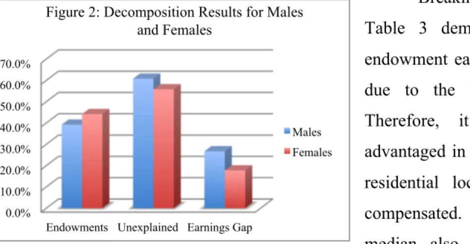
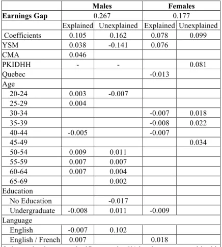
The decomposition results show the wage disadvantage suffered by Visible Minority immigrants compared to White immigrants. Table 3 shows the overall results of the decomposition and coefficients of specific variables that were significant and of a meaningful magnitude (complete results in Table A.3 in the Appendix). Figure 2 is a graphical representation of the percentage explained and unexplained differences in wages. Visible Minority immigrant males earn 26.7% less per hour than White immigrant males. The situation is better for females, but still very large at a 17.7% less for Visible Minorities compared to Whites. Referring to Figure
CMA >500,000 -0.181* 0.0438 -0.193* 0.0527 -0.060 0.0731 -0.178** 0.1000 PKIDHH -0.001 0.0331 -0.098* 0.0259 Region Quebec -0.154* 0.0414 -0.228* 0.0305 -0.343* 0.0639 -0.187* 0.0407 Ontario - - - - Prairies -0.105* 0.0310 -0.065* 0.0224 -0.178* 0.0575 -0.110* 0.0376 British Columbia -0.099* 0.0320 -0.103* 0.0216 -0.044 0.0631 -0.092* 0.0269 Age 18-19 -0.489* 0.1231 -0.294* 0.1354 -0.664* 0.2192 0.004 0.2842 20-24 -0.436* 0.0699 -0.170* 0.0437 -0.444* 0.1097 -0.153* 0.0590 25-29 -0.264* 0.0537 -0.128* 0.0321 -0.077 0.0950 -0.100* 0.0418 30-34 -0.126* 0.0424 -0.076* 0.0264 -0.002 0.0673 -0.066** 0.0361 35-39 -0.098* 0.0356 -0.043** 0.0232 -0.009 0.0543 -0.029 0.0307 40-44 - - - - 45-49 -0.003 0.0324 0.004 0.023 0.013 0.0491 -0.062* 0.0298 50-54 0.022 0.0317 -0.034 0.0258 -0.090** 0.0498 -0.099* 0.0334 55-59 -0.025 0.0339 -0.066* 0.0286 -0.150* 0.0546 -0.139* 0.0399 60-64 -0.035 0.0370 -0.096* 0.0372 -0.128** 0.0682 -0.101 0.0609 65-69 -0.037 0.0685 -0.205* 0.0812 -0.454* 0.1806 -0.017 0.2831 Education No Education - - - - High School 0.177* 0.0271 0.066* 0.0209 0.125* 0.0375 0.038 0.0243 College 0.267* 0.0291 0.152* 0.023 0.279* 0.0434 0.171* 0.0296 Undergraduate 0.425* 0.0343 0.269* 0.024 0.411* 0.0561 0.303* 0.0312 Postgraduate & Professional 0.555* 0.0452 0.418* 0.033 0.471* 0.0699 0.472* 0.0551 Knowledge of Official Language
English - - - -
French -0.141* 0.0614 0.022 0.0469 -0.025 0.0948 -0.049 0.0573 English & French -0.040 0.0373 0.034 0.0354 0.188* 0.0621 0.222* 0.0540 No Official Language -0.295* 0.0796 -0.060** 0.0363 -0.026 0.0871 -0.052 0.0322 Constant 3.051* 0.0597 2.865* 0.0634 2.672* 0.1005 2.737* 0.1005 R2 0.2186 0.2121 0.2290 0.2070 * = significance at 5% level **=significance at 10% level
2, the model could only explain 39.2% of the difference in wages for men, and 44.2% for females. Therefore the wage difference was in large part due to discrimination or unobserved variables.
Breaking down the results further, Table 3 demonstrates that most of the endowment earnings difference for males is due to the YSM and CMA variables. Therefore, it is because Whites are advantaged in terms of years in Canada and residential location, that they are better compensated. Age on both sides of the median also helps to explain the wage discrepancy, except at the median age of 40-44, where Visible Minorities actually have an advantage. Looking at the unexplained component, again YSM was large and significant, but negative (-0.14). This means that the return on being longer in Canada is greater for Visible Minorities than Whites. Age above the median has a lower return for Visible Minorities, but the opposite is true for individuals aged 20-24 years. The largest contributor to the unexplained difference in earnings is the variable English at 0.102. As the total unexplained component is 0.162, English is a large component of the difference in hourly wage, implying that Visible Minorities have a lower return on speaking English than Whites. Henceforth, it is not language skills that are lacking in the Visible Minority population, but the return on these skills.
For females, YSM is also positive and significant, and larger than that of males. Again, Whites have the advantage in terms of years in Canada. Visible Minority females however have an endowment advantage for residing in Quebec, as well as belonging to the age group 30-44, compared to Whites. However, Whites have an endowment advantage over Visible Minorities in terms of speaking both official languages. Looking at the discrimination component, having children is the largest contributing factor for females, indicating that having children has a negative return on Visible Minority female earnings compared to White females. Visible Minorities suffer a lower return on the age groups 30-34 and 35-39, which are two of the age groups in which they have endowment advantages. This could suggest that being of the right age,
0.0% 10.0% 20.0% 30.0% 40.0% 50.0% 60.0% 70.0%
Endowments Unexplained Earnings Gap
Figure 2: Decomposition Results for Males and Females
Males Females
but a Visible Minority, is not enough to satisfy employers to compensate them at the same level as their White peers.
Unconditional Quantile Regression using the Oaxaca-Blinder Decomposition
Unconditional Quantile regression was performed for the 10th, 25th, 50th, 75th, and 90th quantile. This was done in order to ensure a complete picture of where in the wage distribution the earnings gaps lie, and what are their causes. For all the quantiles, the log earnings gaps are significant, however the Table 3
Oaxaca-Blinder Decomposition of Earnings Gap, Partial Results
Males Females
Earnings Gap 0.267 0.177
Explained Unexplained Explained Unexplained Coefficients 0.105 0.162 0.078 0.099 YSM 0.038 -0.141 0.076 CMA 0.046 PKIDHH - - 0.081 Quebec -0.013 Age 20-24 0.003 -0.007 25-29 0.004 30-34 -0.007 0.018 35-39 -0.008 0.022 40-44 -0.005 -0.007 45-49 0.034 50-54 0.009 0.011 55-59 0.007 0.007 60-64 0.007 0.004 65-69 0.002 Education No Education -0.017 Undergraduate -0.008 0.011 -0.009 Language English -0.007 0.102 English / French 0.007 0.018
Only results that were significant at the 5% level were reported in this table, the complete results can be found in the Appendix Table table
0.0% 5.0% 10.0% 15.0% 20.0% 25.0% 30.0% 0.1 0.25 0.5 0.75 0.9
Figure 3: Observed Log Earnings Gap
Males Females
components of these gaps, explained and unexplained, are not significant for females in the 10th quantile at the 5% level (the explained component is significant at the 10% level). The full results for these regressions can be found in Tables A.5 and A.6 of the Appendix.
Figure 3 summarizes the evolution of the wage differential through the quantiles. It is immediately obvious that Visible Minority males continuously suffer higher rates of wage differential than female Visible Minorities. The earnings gaps of males are relatively constant throughout the quantiles, starting at their lowest point at 25.1% less than White males, and reaching a high of 28.2% at the 75th percentile. The female
earnings gap starts at a much lower rate of 9.5% at the 10th quantile, and jumps to a differential of
19.5% at the 25th quantile. After this point, the wage gap is somewhat constant, with a maximum of 21.5% at the median.
Figure 4 represents the unexplained or discrimination portion of the wage gap. It is obvious from the figure that for all the quantiles of both sexes, most of the difference in wage cannot be explained by differences in characteristics. Notice that at the 10th quantile, there are no results for females. This is because, as aforementioned, the unexplained and endowment components are not significant at the 5% level individually for females. Therefore, there is a significant difference in wages between Visible Minorities and White females, but the source of this difference cannot be precisely determined.
Once the female unexplained contribution is significant, it follows the same pattern as the males, and is close in magnitude to the males as well. The U-shaped discrimination portion throughout the quantiles demonstrates that as
wages increase, so does discrimination. However, the magnitude of the discrimination does not fluctuate much overall. For males, the unexplained proportion tends to hover around 60%, and for females a little lower.
Looking more closely at the results of the quantile regressions in Figures 5 through 8,
0.0% 20.0% 40.0% 60.0% 80.0% 0.1 0.25 0.5 0.75 0.9
Figure 4: Unexplained Proportion of Observed Log Earnings Gap
Males Females -0.02 -0.01 0 0.01 0.02 0.03 0.04 0.05 0.06 0.07 0.1 0.25 0.5 0.75 0.9
Figure 5: Partial Results for the Earnings gap due to Characteristic differences
(Males)
YSM CMA Undergraduate
and in detail in Table A.5 and Table A.6 of the Appendix, a different story appears for males and females. Focusing first on Figure 5 for males, where only the large coefficients of variables that are significant are reported, it is obvious that there are two principal factors contributing to the earnings gap, namely YSM and CMA. In the first two quantiles, YSM is
responsible for half of the difference in endowments, while in the middle of the distribution; it is living in a large metropolitan area (CMA) that explains this difference in earnings. Many age groups are significant throughout the earnings distribution, but there is no particular group that can claim to be a principal source of the earnings gap. Visible Minorities have an advantage in endowments in terms of an undergraduate education, and that advantage starts and grows from the 25th quantile onward. Therefore education cannot explain the wage differences in the endowment section, as education reduces the gap.
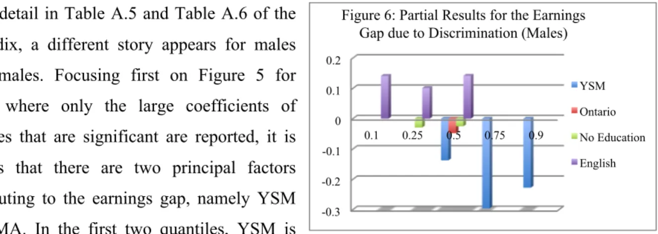
Moving on to Figure 6, the unexplained or discrimination portion, it can be seen that English in the first three quantiles is the principal cause of the unexplained earnings gap. Therefore, the return on being proficient in the English language is far less for Visible Minorities than for Whites. Moving the analysis to the top end of the wage distribution, an overall wage gap above 25% is observed, but no particular variable can explain this difference. This difference is mainly due to the large constants, and only the one belonging to the 75th quantile is significant. This suggests that in the most upper part of the distribution, the selected variables are unable to explain the difference in earnings, and perhaps in these percentiles different factors come into play. What is significant in these quantiles and at the median is YSM. YSM is negative and of a respectable magnitude of up to -0.296, implying that the return on time in Canada is much greater for Visible Minorities than it is for Whites.
Turning to Figures 7 and 8, the explained and unexplained variables that
-0.02 0 0.02 0.04 0.06 0.08 0.1 0.12 0.1 0.25 0.5 0.75 0.9
Figure 7: Partial Results for the Earnings gap due to Characteristic differences
(Females) YSM Quebec Undergraduate English & French -0.3 -0.2 -0.1 0 0.1 0.2 0.1 0.25 0.5 0.75 0.9
Figure 6: Partial Results for the Earnings Gap due to Discrimination (Males)
YSM Ontario No Education English
contribute to the wage gap for females are displayed. The principal variable contributing to the difference in endowment was YSM, much like the males. For all except the highest quantile, Whites have an advantage when it comes to the years they have spent in Canada. Quebec’s coefficients are negative and significant at the 5% level for the four lower quantiles, indicating that Visible Minorities are advantaged in terms of their region. Visible Minority women are also more advantaged in terms of the age group they belong to for the first three quantiles. The education variable Undergraduate is negative and significant for the top four quantiles, suggesting Visible Minority females have superior endowments in terms of undergraduate education compared to Whites. Finally, White females have a characteristic advantage over Visible Minority females in terms of being proficient in both official languages, which is significant at the 5% level for the first three quantiles, and significant at the 10% level in the 75th
quantile.
Turning attention to Figure 8, which displays the unexplained wage gap portion for females; the causes were not as clear as for the explained component. In the first two quantiles, both Ontario and multiple age groups have worse returns for Visible Minorities than Whites. Therefore residing in Ontario and being a Visible Minority female has a negative effect on the individual’s wage. Curiously, only at the median is living in a central metropolitan area a point of large discrimination for women, as it is not significant in any other quantile. Finally, in the 75th quantile, having children has a much lower return for Visible Minority females, than for White
females. The coefficient is large at 0.191, given that the total magnitude of the unexplained portion is only 0.105. The variable PKIDHH is significant only at the 10% level in the 90th quantile, but is smaller than the 75th quantile’s, at 0.131. Therefore the negative wage consequences for Visible Minority females are only a problem for those in the highest quantiles.
-0.05 0 0.05 0.1 0.15 0.2 0.25 0.3 0.35 0.1 0.25 0.5 0.75 0.9
Figure 8: Partial Results for the Earnings Gap due to Discrimination (Females)
CMA PKIDHH Quebec Ontario
5. Discussion
This study finds that earnings gaps do exist between White and Visible Minority immigrants of both sexes, but that the differential is larger for males. These findings are consistent with the previous literature from Pendakur and Pendakur (1998) and Swidinsky and Swidinsky (2002). However, the current results demonstrate that there is a greater wage gap in the manufacturing industry, than in the general Canadian economy. Both previous studies found a 14% earnings gap for males, while the current findings demonstrate a 26.7% earnings gap in the manufacturing sector. This implies that Visible Minority males in manufacturing receive 12% less per hour than the average Visible Minority male immigrant salaried worker in Canada. The previous literature for females found a 7.4% wage gap in 1991, and 2.9% wage gap in 1996. The results for manufacturing found in the current study suggest Visible Minority females suffer a 17.7% earnings gap, henceforth experiencing an added 10% earnings deficit to the one previously found by Swidinsky and Swidinsky (2002) using 1996 data, which looked at all industries.
Comparing the coefficients from the four OLS log-earnings regressions with the previous literature of Swidinsky and Swidinsky, many similarities are seen. YSM is positive and significant for all the sexes and races in both studies. Both the previous and current work find that
Marital Status is significant mainly for males, and has a greater return for Whites, as well as the
same return pattern on the variable Quebec. However, unlike the current study, Undergraduate was not significant for White males, and had a greater return for Visible Minority females in the Swidinsky and Swidinsky study. In the present work, Undergraduate is significant for each group, and Whites altogether have a greater return on an undergraduate degree than Visible Minorities. The Swidinsky and Swidinsky study also found that not speaking any official language was significant for all groups except Visible Minority males; the current study findings are much less significant for the language variables. Immigrants are heavily concentrated in semi-skilled manual work positions (Females: 35% of Whites and 47% of Visible Minorities; Males: 26% of Whites and 46% of Visible Minorities). These positions do not necessarily demand significant language skills, which could explain the difference in significance of these variables between the two studies.
These results demonstrate the differences and similarities of the manufacturing industry to the whole Canadian economy. Language proficiency is not as important in manufacturing as in
other industries, and an undergraduate degree is undervalued for Visible Minorities in manufacturing. This difference may be due to the dissimilar job positions that Visible Minorities immigrants hold in other industries compared to manufacturing.
This is the first study to conduct a quantile regression analysis on wage discrimination between White and Visible Minority immigrants in the Canadian manufacturing sector. Discrimination is relatively constant throughout the entire wage distribution, and males continuously face a larger wage gap. However, the causes for the earnings gap cannot be completely attributed to one factor. Looking first at the endowment component of the wage differential, YSM is a very important explanatory factor in the lower part of the wage distribution for both sexes. However, YSM becomes irrelevant, especially for males, in the upper most quantiles. Although CMA and age can explain much of the wage differential in the middle of the distribution, these factors become irrelevant at the top of the distribution. Unionization is highest in small CMAs and rural areas (Bernard, 2009), and unionization has a positive impact on wages (Doiron & Riddell, 1994). Given that the percentage of White immigrants in non-CMAs is much higher than Visible Minorities immigrants, it is perhaps because they are unionized that CMA is significant. However, CMA and age contribute less for females. Age overall actually reduces the wage gap due to characteristic differences for females.
In the unexplained portion of the wage gap, only English is an important contributor to the earnings gap for males, and only in the first three quantiles. The importance of this variable may be due to the difference in quality of English spoken between the two groups. Tainer (1988) found that the quality of English spoken and the region of origin of the individual has different effects on earnings in the United States. Tainer controlled for the quality of English spoken, and found that European immigrants from non-English countries (whose citizens are typically White) had higher earnings than immigrants from Hispanic and Asian countries. This suggests that speaking with an accent played an active role in wage determination. Tainer also found that after controlling for region of origin, those with better language skills were better compensated. Therefore, if it had been possible to include a variable that took into account the level of language proficiency, a more complete appreciation of the return on language could have been gained.
Although the contributors to discrimination are not constant for females, there exists large significant variables that are sources of discrimination. Overall the 10th quantile is not significant, but Age and Ontario are, and these variables continue to be in the next quantile. Age is not a skill
that can be learned or changed, and is a true point of discrimination. Ontario’s significance in the unexplained component could partly be attributed to the type of manufacturing that exists in Ontario, compared to other parts of the country. CMA is only significant but very large at the 50th quantile. Unionization is highest in small CMAs, and unionization usually produces higher wages. If the positions that are in the 50th quantile are located outside of the large urban areas, where there are more White immigrants, then this could explain the significance of the CMA variable. In the presence of a unionization variable, perhaps CMA would no longer be significant, and the unionization variable would be significant and in the explained portion of the earnings gap.
Finally, having children are the contributing factor to the wage differential in the two upper most quantiles. Here, the vagueness of this variable could be the cause of its prevalence in the discrimination component, as it only registers the existence of children, not the number of children. If the difference between the number of children that White and Visible Minorities females have were significant, then the discrimination portion of the wage gap due to this variable could become a feature of the endowment earnings differential. Another explanation of the significance of the variable PKIDHH could be the different cultural demands of Visible Minority mothers compared to White mothers. To effectively capture this divergence in culture, the analysis would need to account for the country of origin of both White and Visible Minorities females, as well as the number of children these individuals have. Given the small number of observations for many of the different ethnicities present in the manufacturing industry, the robustness of such an analysis would be questionable. To examine the children factor in depth, a more economy-wide analysis would need to be performed.
What is apparent for both sexes is the inability of the model to explain the earnings gap in the upper quantiles. There is no variable that can explain the wage gap for males in the last two quantiles, and only one factor at the 75th quantile for females. This lack of explanatory factors demonstrates the weakness of the model in these quantiles, and the different reality that define the high earners of the manufacturing industry. Including such variables as job tenure, occupation, unionization, firm size, and whether the company is publicly or privately owned could help mitigate the problem. If differences exist in the distribution and return for Whites and Visible Minorities in the previously listed categories, then the earnings gap could perhaps be better explained.
6. Conclusion
The face of Canada is changing, and how Visible Minority immigrants are treated in Canadian society is an increasingly mainstream concern. The present study demonstrates the earnings deficit Visible Minority immigrants suffer throughout the wage spectrum. Males are the greater victims of the two sexes, but both suffer the same rate of wage discrepancy due to discrimination. The causes of the earnings gap are not due to one particular characteristic, making it hard to create a policy that relieves the issue. Years Since Immigration is the most significant variable of large magnitude throughout the endowment portion of the wage differential. The usefulness of this variable in policy creation is minimal, as the only possible cure is time itself. An interesting future study would be to examine different YSM quantiles through an Oaxaca-Blinder Decomposition. Doing so would perhaps demonstrate how many years in Canada are needed for earnings of Visible Minorities and Whites to be equal.
The next step in a study such as this one would try to correct for selection problems. For males and females, this would take into account that employers discriminate at hiring, therefore either not hiring certain individuals due to race or accent, or offering a position below the skill level of the individual, because they belong to a Visible Minority. Another instance where it could be possible to control for selection bias is the labor supply of Visible Minority females. If the cultural backgrounds of Visible Minority groups discourage females from entering the work force, only those with relatively high skills would do so, as the return to those with low skills would be too low given their cultural beliefs. However, this could be true for White immigrants as well, therefore controlling for selection bias could drastically change the outcome.
The present market conditions create a disincentive for Visible Minorities to join the workforce and contribute to the Canadian economy wholeheartedly. If we continue to fail to assimilate the largest proportion of immigrants into the workforce, we have defeated one of the principal purposes of immigration policy itself.
Bibliography
Baker, M., & Benjamin, D. (1994). The Performance of Immigrants in the Canadian Labor Market. 12 (3), 369-‐405.
Beach, C., & Worswick, C. (1993). Is There a Double Negative Effect on Earnings of Immigrant Women? Canadian Public Policy/Analyse de Politique , 19 (1), 36-‐53. Bernard, A. (2009). Trends in manufacturing employment. Ottawa: Statistics Canada.
Blinder, A. S. (1973). Wage Discriminaton: Reduced Form and Structural Estimates. Journal
of Human Resources , 8 (4), 436-‐455.
Bonnal, L., Boumahdi, R., & Favard, P. (2013). The easiest way to estimate the Oaxaca– Blinder decomposition. Applied Economics Letters , 96-‐101.
Boudarbat, B., & Lemieux, T. (2010). Why are the Relative Wages of Immigrants Declining? A
Distributional Approach. Vancouver: Canadian Labour MArket and Skills Research Network.
Boudarbat, B., Pray, & Connolly, M. (2011). L’écart salarial entre les sexes chez les nouveaux
diplômés postsecondaires . L’écart salarial entre les sexes chez les nouveaux diplômés
postsecondaires : CIRANO.
Christofides, L., & Swidinsky, R. (1994). Wage Determination by Gender and Visible Minority Status: Evidence from the 1989 LMAS. Canadian Public Policy -‐ Analyse de
Politiques , 34-‐51.
DeSilva, A. (1992). Earnings of immigrants: A comparative analysis. Ottawa, Canada: Economic Council of Canada.
Doiron, D. J., & Riddell, W. C. (1994). The Impact of Unionization on Male-‐Female Earnings Differences in Canada. The Journal of Human Resources , 29 (2), 504-‐534 .
Firpo, S., Fortin, N., & Lemieux, T. (2009). Unconditional Quantile Regressions. Econometrica
, 77 (3), 953-‐973.
Fortin, N., Lemieux, T., & Firpo, S. (2010). Decomposition Methods in Economics. National Bureau of Economic Research, Working Paper No 16045.
Frank, K., Phythian, K., Walters, D., & Anisef, P. (2013). Understanding the Economic Integration of Immigrants: A Wage Decomposition of the Earnings Disparities between Native-‐Born Canadians and Recent Immigrant Cohorts. Social Sciences , 40-‐61.
Gardeazabal, J., & Ugidos, A. (2005). Gender wage discrimination at quantiles . Journal of
Population Economics , 165-‐179.
Gardeazabal, J., & Ugidos, A. (2004). More On Identification In Detailed Wage Decompositions. The Review of Economics and Statistics , 1034-‐1036.
Hum, D., & Simpson, W. (1999). Wage Opportunities for Visible Minorities in Canada.
Canadian Public Policy -‐ Anallyse De Politiques , 45 (3), 379-‐394.
Jann, B. (2008). A Stata implementation of the Blinder-‐Oaxaca decomposition. The Stata
Journal , 453-‐479.
Li, P. S. (2000). Earning Disparities between Immigrants and Native-‐born Canadians.
Canadian Review of Sociology/Revue canadienne de sociologie , 37 (3), 289-‐311.
Munro, M. J. (2003). A Primer on Accent Discrimination in the Canadian Context. TESL
Canada Journal , 20 (2), 38-‐51.
Neumark, D. (1988). Employers' Discriminatory Behavior and the Estimation of Wage Discrimination. 23, 279-‐295.
Oaxaca, R. L., & Ransom, M. R. (1999). Identification In Detailed Wage Decomposition. The
Oaxaca, R. (1973). Male-‐female Wage Differentials in Urban Labor Markets. International
Economic Review , 693-‐709.
Pendakur, K., & Pendakur, R. (1998). The colour of money: earnings differentials among ethnic groups in Canada. Canadian Journal of Economics , 518-‐548.
Suits, D. B. (1984). Dummy Variables: Mechanics V. Interpretation. The Review of Economics
and Statistics , 177-‐180.
Swidinsky, R., & Swidinsky, M. (2002). The Relative Earnings of Visible Minorities in Canada: New Evidence from the 1996 Census. Relations industrielles / Industrial Relations ,
57 (4), 630-‐659.
Tainer, E. (1988). English Language Proficiency and the Determination of Earnings among Foreign-‐Born Men . The Journal of Human Resources , 23 (1), 108-‐122.
Vartiainen, J. (2002). Gender wage differentials in the Finnish labour market. Helsinki: Ministry of Social Affairs and Health.
Yun, M.-‐S. (2005). A Simple Solution To The Identification Problem In Detailed Wage Decompositions. Economic Inquiry , 43 (4), 766-‐772.
Appendix
Figure A.1: Female Log Wage Distribution
Bands represent 10 centiles
Figure A.2: Male Log Wage Distribution
Bands represent 10 centiles
0 .2 .4 .6 .8 1 1.69 2 3.5 5.1 Female Log(Wage)
Visible Minority White
0 .2 .4 .6 .8 1.69 2 3.5 5.1 Male Log(Wage)
Table A.1: OLS Log Earnings Estimation with Visible Minority Variable for Males and Females
Males Females
Variables Coef. Std. Err. Coef. Std. Err.
YSM 0.006 0.0010 * 0.007 0.002 * Age at Immigration -0.003 0.0005 * -0.002 0.001 * Interaction 0.006 0.0011 * 0.005 0.002 * Marital Status 0.070 0.0144 * -0.042 0.019 * CMA -0.221 0.0317 * -0.135 0.054 * PKIDHH - - - -0.054 0.020 * Quebec -0.201 0.0247 * -0.245 0.034 * Prairies -0.080 0.0183 * -0.137 0.031 * BC -0.096 0.0180 * -0.092 0.025 * age18_19 -0.417 0.0906 * -0.478 0.169 * age20_24 -0.263 0.0373 * -0.235 0.052 * age25_29 -0.174 0.0277 * -0.108 0.038 * age30_34 -0.105 0.0225 * -0.062 0.032 ** age35_39 -0.064 0.0196 * -0.031 0.027 age45_49 0.005 0.0189 -0.035 0.026 age50_54 -0.003 0.0200 -0.087 0.028 * age55_59 -0.045 0.0217 * -0.151 0.032 * age60_64 -0.068 0.0255 * -0.123 0.044 * age65_69 -0.112 0.0517 * -0.351 0.147 * High School 0.111 0.0167 * 0.066 0.020 * College 0.204 0.0181 * 0.212 0.024 * Undergraduate 0.323 0.0197 * 0.335 0.027 * Postgraduate & Professional 0.473 0.0268 * 0.467 0.043 * French -0.028 0.0374 -0.030 0.049 English & French 0.012 0.0251 0.185 0.038 * No Official Language -0.095 0.0333 * -0.054 0.030 ** Visible Minority -0.141 0.0129 * -0.053 0.019 * Constant 3.084 0.0416 * 2.762 0.067 * R-Squared 0.2544 0.2248 Number of Observations 6311 2816 * = Significance at 5% level ** = Significance at 10% level
Table A.2: OLS Log Earnings Estimation with Interaction Terms For Males and Females
Males Females
Variables Coef. Std. Err. Coef. Std. Err. YSM 0.004 0.0012 * 0.008 0.0020 * Age at Immigration -0.002 0.0008 * -0.002 0.0013 ** Interaction 0.005 0.0014 * 0.003 0.0023 Marital Status 0.095 0.0227 * -0.038 0.0339 CMA -0.181 0.0427 * -0.060 0.0703 PKIDHH -0.001 0.0318 Quebec -0.154 0.0403 * -0.343 0.0615 * Prairies -0.105 0.0302 * -0.178 0.0553 * BC -0.099 0.0312 * -0.044 0.0607 age18_19 -0.489 0.1200 * -0.664 0.2109 * age20_24 -0.436 0.0681 * -0.444 0.1055 * age25_29 -0.264 0.0524 * -0.077 0.0914 age30_34 -0.126 0.0413 * -0.002 0.0648 age35_39 -0.098 0.0347 * -0.009 0.0522 age45_49 -0.003 0.0316 0.013 0.0472 age50_54 0.022 0.0309 -0.090 0.0479 ** age55_59 -0.025 0.0330 -0.150 0.0525 * age60_64 -0.035 0.0361 -0.128 0.0656 ** age65_69 -0.037 0.0668 -0.454 0.1738 * High School 0.177 0.0264 * 0.125 0.0361 * College 0.267 0.0284 * 0.279 0.0418 * Undergraduate 0.425 0.0335 * 0.411 0.0540 * Postgraduate & Professional 0.555 0.0440 * 0.471 0.0673 * French -0.141 0.0598 * -0.025 0.0912 English & French -0.040 0.0364 0.188 0.0598 * No Official Language -0.295 0.0776 * -0.026 0.0838 Visible Minority -0.187 0.0868 * 0.065 0.1500 YSM-V 0.009 0.0027 * 0.000 0.0049 Age at Immigration-V 0.000 0.0011 0.003 0.0051 Interaction-V -0.001 0.0028 0.001 0.0017 Marital Status-V -0.027 0.0293 0.005 0.0407 CMA-V -0.012 0.0686 -0.118 0.1239 PKIDHH-V -0.097 0.0414 * Quebec-V -0.074 0.0509 0.156 0.0741 * Prairies-V 0.040 0.0378 0.068 0.0673
BC-V -0.004 0.0381 -0.047 0.0666 age18_19-V 0.195 0.1827 0.668 0.3584 ** age20_24-V 0.265 0.0813 * 0.291 0.1214 * age25_29-V 0.136 0.0617 * -0.023 0.1008 age30_34-V 0.050 0.0493 -0.064 0.0745 age35_39-V 0.056 0.0420 -0.020 0.0609 age45_49-V 0.007 0.0393 -0.075 0.0561 age50_54-V -0.056 0.0406 -0.009 0.0587 age55_59-V -0.042 0.0440 0.011 0.0664 age60_64-V -0.061 0.0522 0.027 0.0903 age65_69-V -0.168 0.1062 0.437 0.3369 High School-V -0.111 0.0339 * -0.087 0.0438 * College-V -0.115 0.0368 * -0.108 0.0515 * Undergraduate-V -0.156 0.0414 * -0.107 0.0626 ** Postgraduate & Professional-V -0.137 0.0553 * 0.001 0.0876 French-V 0.162 0.0765 * -0.025 0.1083 English & French-V 0.075 0.0512 0.034 0.0813 No Official Language-V 0.234 0.0859 * -0.025 0.0900 Constant 3.051 0.0582 * 2.672 0.0967 * R-squared 0.2684 0.2402 Number of observations 6311 2816 * = Significance at 5% level ** = Significance at 10% level
Table A.3: Oaxaca-Blinder Decomposition for Males and Females
Males Females
Coef. Std. Err. Coef. Std. Err.
Differentia: LN Hourly Wage
Prediction_1 3.229 0.0100 * 2.842 0.0159 * Prediction_2 2.962 0.0076 * 2.664 0.0102 * Difference 0.267 0.0126 * 0.177 0.0189 * Explained YSM 0.038 0.0128 * 0.076 0.0210 * Age at Immigration -0.002 0.0009 * -0.003 0.0019 Interaction 0.010 0.0034 * 0.010 0.0080 Marital Status 0.001 0.0010 -0.001 0.0013 CMA 0.046 0.0114 * 0.013 0.0158 PKIDHH 0.000 0.0056 Quebec -0.002 0.0012 ** -0.013 0.0044 * Ontario 0.001 0.0011 0.003 0.0027 Prairies 0.000 0.0003 0.000 0.0004 BC 0.000 0.0008 -0.008 0.0043 ** age18_19 -0.001 0.0007 -0.002 0.0013 age20_24 0.003 0.0014 * 0.003 0.0019 age25_29 0.004 0.0016 * -0.004 0.0036 age30_34 0.000 0.0017 -0.007 0.0030 * age35_39 -0.002 0.0017 -0.008 0.0032 * age40_44 -0.005 0.0016 * -0.007 0.0033 * age45_49 -0.002 0.0013 -0.002 0.0030 age50_54 0.009 0.0021 * 0.004 0.0025 ** age55_59 0.007 0.0019 * 0.003 0.0041 age60_64 0.007 0.0021 * 0.002 0.0028 age65_69 0.001 0.0008 -0.002 0.0012 No Education 0.001 0.0027 0.000 0.0046 High School -0.003 0.0014 * 0.000 0.0025 College -0.001 0.0007 0.001 0.0010 Undergraduate -0.008 0.0018 * -0.009 0.0030 * Postgraduate & Professional -0.002 0.0017 0.005 0.0022 * English -0.007 0.0021 * 0.001 0.0015 French 0.000 0.0002 0.001 0.0008 English & French 0.007 0.0027 * 0.018 0.0055 *