HAL Id: hal-01354303
https://hal.archives-ouvertes.fr/hal-01354303
Submitted on 5 Mar 2019
HAL is a multi-disciplinary open access
archive for the deposit and dissemination of
sci-entific research documents, whether they are
pub-lished or not. The documents may come from
teaching and research institutions in France or
abroad, or from public or private research centers.
L’archive ouverte pluridisciplinaire HAL, est
destinée au dépôt et à la diffusion de documents
scientifiques de niveau recherche, publiés ou non,
émanant des établissements d’enseignement et de
recherche français ou étrangers, des laboratoires
publics ou privés.
Cooling channel optimization for injection molding
Nicolas Pirc, Florian Bugarin, Fabrice Schmidt, Marcel Mongeau
To cite this version:
Nicolas Pirc, Florian Bugarin, Fabrice Schmidt, Marcel Mongeau. Cooling channel optimization for
injection molding. NUMIFORM 07: Materials Processing and Design: Modeling, Simulation and
Applications, Jun 2007, Porto, Portugal. p.525-530, �10.1063/1.2740864�. �hal-01354303�
Cooling channel optimization for injection molding
N.Pirc
1, F. Bugarin
1, F.M. Schmidt
1, M.Mongeau
21CROMeP - Ecole des Mines d’Albi Carmaux
Campus Jarlard – 81013 Albi, Cedex 09, France URL: : http://www.enstimac.fr/recherche/cromep
2Université de Toulouse, LAAS- CNRS - 7 avenue du Colonel Roche
31077 Toulouse Cedex 4, France URL: www.mip.ups-tlse.fr/~mongeau
Abstract. In injection molding process, heat transfer during the cooling step plays an important role. This step has a
great influence on the quality of the final parts that are produced, as well as on the molding cycle time. We introduce an optimization procedure in order to locate automatically the cooling channels in 3D injection molds. The temperature distribution is computed using the Boundary Elements Method (BEM) that allows reducing the computation space from 3D to 2D, (avoiding full 3D remeshing). In our study, BEM is used to solve the stationary heat conduction problem. The BEM heat transfer solver is coupled with the non-linear optimization algorithm SQP (Sequential Quadratic Programming). The SQP algorithm permits to calculate the best set of cooling parameters, for a given cost function. For example, one such cost function involves minimizing the temperature variations at the interface between the mold cavity and the polymer. We present preliminary 3D computational results.
Keywords: BEM, heat transfer, injection molding, mold-cooling simulation, optimization, SQP. PACS: 02.70.Pt
INTRODUCTION
Numerical simulations are more and more used for designing injection molds. The location of the cooling channels is a major element in the design of the mold because the cooling time can represents up to 70% of the injection cycle. Rapid prototyping processes such as layered design or selective laser sintering start to be used to manufacture injection molds. The advantage of these assembling processes is the possibility to obtain almost any desired shape of mold geometry. However; it is then more difficult to locate and to shape the cooling channels. Numerical simulation can be used to perform automatic optimization of the position and the shape of the cooling channels.
Simulation of Heat Transfer during
Injection Mold
Numerical simulation is used to solve the heat balance equation and evaluate a cost (or objective) function related to part quality and/or productivity. Several numerical methods such as Finite Element
Method (FEM) [1] or Boundary Element Method (BEM) [2] can be used. Using BEM makes it possible to reduce by one the dimension of the mesh involved, meshing only the contour surface.
Mold-Cooling Optimization Approaches
The modeling of the heat transfer using BEM makes it possible to re-mesh only the surface of the channels during the optimization. An optimization method is used to modify the location and shape parameters of the channels and improve the cooling performance of the mold.L. Silva [3] uses 3D FEM software to model injection molding cycle for complex geometries of molds. However, the computational burden of the 3D renders the integration of optimization difficult.
Mathey [4] used 2D stationary and transient BEM simulations of injection molds coupled with an SQP algorithm (Sequential Quadratic Programming) [5] to improve mold injection cooling.
In this paper, we extend Mathey’s approach in view of addressing 3D optimization. An other
contribution is the improvement of the optimization formulation. We perform numerical simulations on a semi-industrial injection mold designed for the European project: Eurotooling 21. We optimize cooling channel locations on both 2D and 3D models. We attempt at minimizing the maximal cooling temperature of the plastic part subject to a temperature uniformity constraint.
STATIONARY HEAT TRANSFER
PROBLEM
The variation of the temperature in the injection mold in production, after some cycle, is a quasi-stationary mode. After the average temperature of the mold during a cycle is stabilized (Fig. 1), we consider a stationary regime. We neglect the transitory oscillations of the temperature.
FIGURE 1. Schematic temperature evolution in injection
mold during several cycles.
Solving Heat Balance Equation using
Boundary Elements Method
The stationary heat conduction problem assuming constant thermal conductivity reduces to Laplace equation.
€
ΔT = 0 (1)
Multiplying this equation by a weighting function T*, and using Green’s theorem, we obtain the well-known Somigliana’s equation [6]:
€ C.T P
( )
+ T. ∇T(
*.n)
.dΓ Γ ∫ =(
∇T.n)
.T*.dΓ Γ ∫ (2)T is the temperature, and C is equal to 1 inside the
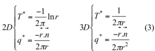
domain and to 0.5 on its regular boundary. T* and q* denotes the fundamental solutions of the problem so-called Green’s functions [6]:
€ 2D T*= −1 2π lnr q*=−r.n 2πr 3D T*= 1 2πr q*= −r.n 2πr2 (3)
After reorganization of equation (2), we obtain a non-symmetrical linear system.
Boundary Conditions
Figure 2 displays the boundary conditions on the mold.
FIGURE 2. Boundary conditions for the mold.
The temperature of the coolant is TC and the heat
transfer coefficient, h, is related to the coolant flow rate (via Colburn correlation coefficient).
€
−λ ∇T .n = h T − T
(
C)
(4)On the cavity surface, the flux density is calculated from the cycle time and polymer properties (heat due to polymer crystallization is neglected) [8].
Thermo Physical Parameters
All the parameters necessary for the numerical heat transfer simulations are referenced in Table 1.
TABLE 1. Thermo physical parameters for the mold and
polymer.
Polymer (PP) Mold (steel 40cmd8s)
λ [ W.m-1.K-1] 0.63 34
ρ [Kg.m-3] 891 7800
Cp [J.Kg-1.K-1] 2740 460
External mold:
Adiabatic condition Cooling channels surface: Convection
Cavity surface: constant flux imposed
Front face Back face
TABLE 2. Process parameters T°C of injection = 240°C T°C of ejection = 100°C Time of injection = 20 s
Mold Cooling Optimization
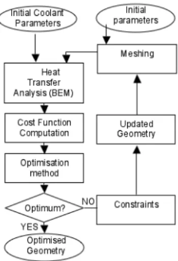
Figure (3) displays the coupling between the thermal solver and the optimization algorithm. Heat transfer computation is coupled with optimization method in order to modify automatically parameters. BEM simulation is performed and cost function is computed. The optimization method allows updating parameters with respect to constraints until a minimum of the cost function is reached. Matlab® SQP, based on the Newton method, is used for the optimization of continuous linear functions with continuous non-linear constraints.
FIGURE 3. Heat transfer simulation coupled with
optimization algorithm.
Cost Function and Constraints
SQP algorithm minimizes just one objective. One method can consider the cost function as the weighting of two objectives, but this method imposes to choose a weighting coefficient. We propose to use the first objective as an optimization criterion (5), and the second as a non-linear constraints (eq 6):€ Φ = max(T) (5) € and 0 ≤ (Ti− Tmoy)2 i ∑ ≤ 4 (6)
The first criterion is the maximum of the temperature on the cavity surface (5).
The second criterion (6) improves the uniformity. For that, Park [9] proposes to minimize the variation of temperature distribution on the cavity surface compared to its average temperature. This function is defined as non-linear constraints. The final configuration provides an uniform and high average temperature, which give a very long cooling time.
Optimization Parameters
In this paper, we consider circular cooling channels in 2D and cylinder in 3D, 3 parameters are needed to describe each cooling channel. Our methodology can also account for optimizing non-linear geometries parameters. These processing parameters can define for instance the thermal regulation: temperature and flow rate of the coolant.
APPLICATION 1: RESULTS FOR A 2D
CASE
In order to validate our approach, we consider the 2D injection geometry as described in Table 1 and 2.
Geometrical Parameters
Our methodology allows for various industrials constraints such as the definition of forbidden zones where one cannot put the cooling channels (due for the presence of the ejectors, or to keep the cooling channel within the mold, or to avoid inter-channel collisions). δ
is the possible displacement according to axis X and Y for the channels.
FIGURE 4. Definition of the geometry parameters.
Forbidden zones delta delta Channel i X (cm) Y (cm) (Xi,Yi)
δ
δ
Numerical Parameters
TABLE 3. Numerical parameters for 2D geometry.
Elements type Linear
Number of elements 1013
Number of nodes 1014
Number of internal nodes 489
Optimization Parameters
Recall that the stationary BEM is used to evaluate the objective function at the mold cavity surface.
The optimization parameters for the locating of the ith cooling channel are (xi,yi) (see Figure 4). Thus, this
2D problem involves 16 optimization variables.
TABLE 4. Channels positions before and after
optimization.
Initial values Final values Channel « i » X Y X Y 1 0.135 0.018 0.129 0.014 2 0.11 0.018 0.106 0.014 3 0.067 0.018 0.063 0.014 4 0.05 0.018 0.046 0.0198 5 0.037 0.049 0.033 0.045 6 0.067 0.049 0.063 0.05 7 0.1 0.049 0.0984 0.0459 8 0.14 0.049 0.136 0.0496
TABLE 5. CPU timed for the direct 2D computing and the
optimization.
Meshing Matrix Aconstruction Solving thesystem Internalspoints computing
0.75 s 1.2188 s 0.64063 s 11.0313 s
The Table 5 displays the CPU time repartition for a direct computing. The matrix construction represents 45% of the direct computing.
FIGURE 5. Objective function versus iterations.
TABLE 6. CPU time for the 2D optimization problem Optimization
time Iterations Number of cost functionevaluations
1320 s 17 367
As illustrated Figure 5, after only 3 optimizations iterations, the objective-function value is already within 5% from the final (optimized) value. The cost function is divided by the initial value to insure 0 ≤
φ
≤ 1.FIGURE 6. Temperature at the surface of the 2D mold
cavity before and after optimization.
Figure 6 displays the temperature distribution along the mold cavity surface before and after optimization. We observe that both temperature variance and temperature average decreased significantly. Figure 7 shows the temperature distribution inside the mold temperature.
FIGURE 7. Temperature distribution after optimization for
the 2D approach.
Front face
Back face
Before
optimization
After
optimization
APPLICATION 2: SIMPLIFIED
APPROACH 3D
We now report computational results on a 3D plastic part whose features are displayed on Figure 8 (unit in mm). The forbidden zones and the input data are identical to those of the 2D case.
FIGURE 8. Schema of plastic part.
Meshing Parameters
The data for the mesh are reported in Table 7.TABLE 7. Meshing parameters for 3D geometry.
Elements type Linear
Number of elements 3266
Number of nodes 3204
The geometrical optimization parameters are now the coordinates of points P1 and P2 (see Figure 9).
The shape of the channels is assumed to be cylindrical and to have a rigid-body motion. Indeed, P2 can then be expressed in terms of P1 coordinates and of the constant channel length L (Figure 9):
FIGURE 9. Channel geometric parameters.
Thus, the optimization parameters for positions of the ith cooling channel are xi, yi, zi. Our 3D problem
therefore involves 24 optimization variables.
TABLE 8. channels positions before and after
optimization.
Initial values Initial values
Channel X Y X Y 1 0.135 0.018 0.131 0.021 2 0.11 0.018 0.101 0.02 3 0.067 0.018 0.058 0.02 4 0.05 0.018 0.046 0.019 5 0.037 0.049 0.033 0.045 6 0.067 0.049 0.063 0.05 7 0.1 0.049 0.0984 0.0459 8 0.14 0.049 0.136 0.0496
Table 9 displays the CPU time for a direct computational. The matrix construction represent 80% of the CPU time for the direct computing.
TABLE 9. CPU time for the direct 2D computing and the
optimization.
Meshing Matrix Aconstruction Resolutionof the system
CPU total
0.75 s 72.21 s 13.295s 86.145 s
Table 10 displays the CPU time optimization.
TABLE 10. CPU time for the 2D optimization. Optimization
time Iterations
Evaluation’s number of the cost function
13.5 H 24 576
Sensibility of the Cost Function
As is illustrated Figure 10, the speed convergence of the cost function is fast.FIGURE 10. Objective function versus iterations.
As it is illustrated in Figure 10, the form of the convergence of the cost function is fast. The value of the cost function is reduced by 90% in 4 iterations. SQP cannot respecting the constraints during optimization if the converge more quickly. This is an advantage in the industrials problems because an initial location of the channels, respecting all the P1(xi,yi,zi)
L
P2(xi,yi,zi)X
Z
Y
φ
iterations
P2 = (X1,Y1,Z1+L) P1=(X1,Y1,Z1) 112 40 22 30° 13
Iterationsφ
constraints, is something difficult to find. This advantage can be a problem if the user considers the accuracy of the convergence sufficient and will stop optimization,
Temperature Distribution
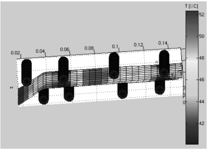
Figure 11 displays the temperature gradient of the surface of mold cavity. The results are similar to 2D geometry, except for the boundary effect.
FIGURE 11. Surface temperature distribution at the surface
of the mold cavity.
CONCLUSION
The BEM has been used to solve heat transfer equation during the cooling step of the molding process, for a 2D and 3D problem. This model is coupled with SQP optimization algorithm to find the best geometrical parameters according to a cost function. SQP is a mono-objective algorithm but it is possible to define one of the objectives like non-linear constraints. It is crucial to study the parameterization of the channels to reduce optimization variable and thus CPU time. The use of the elliptical cooling channels should be further investigated for more complex shapes in future works.
ACKNOWLEDGMENTS
This study was conducted within the frameworks of EUROTOOLING 21 (www.eurotoolin21.com, IP 505901-5).
NOMENCLATURE
M, P and C indexes refer respectively to the mold, the polymer part and the coolant.
C: Heat capacity [J.Kg-1.K-1]
d: Cooling channel diameter [m] h: Heat transfer coefficient [W.m-2.K-1]
S: Surface [m2]
q: Temperature gradient [K.m-1]
R: Thermal contact resistance [K.m2.W-1] Tc : Temperature of the coolant [s] T: Temperature [°C] V: Volume [m3] λ: Thermal conductivity [W.m-1.K-1] Φ: Heat flux [W.m2] ρ: Mass density [Kg.m-3]
REFERENCES
1. Boillat E., Glardon R., Paraschivescu R., “Journal de Physique”, IV, 102, p 27-38 (2002).
2. Polynkin A., international polymer processing, volume XIX, p108-418, 2004.
3. Silva L., international polymer processing, IPP 1888, 2005.
4. Mathey E., AIP Conference Proceedings, Volume 712, pp. 222-227 (2004), NUMIFORM 2004 , ISBN : 0-7354-0188-8..
5. “Optimization Toolbox For Use With Matlab”, The MathWorks (2002) User’s Guide, Version 2. 6. Brebbia C., Domiguez J., “Boundary elements an
introduction of course”, WIT Press/Computational Mechanics Publication, 1992.
7. PARK S.J., International journal for numerical methods in engineering, 43, 1109-1126, 1998
8. JUI-MING L., “Multi-objective optimization scheme for quality control in injection molding”, journal of injection molding technologie, Vol 6, No. 4, December 2002. 9. Wen-Hsien Y., “integrated numerical simulation of
injection molding using true 3D aproch”, ANTEC 2004. 10. WEN-Hsien Y., “integrated numerical simulation of
injection molding using true 3D approach” ANTEC 2004, p486-490