Spouses, Children and Entrepreneurship
⇤
João Galindo da Fonseca
†Charles Berubé
‡March 4, 2020
Abstract
We develop a model of endogenous entrepreneurship and marriage. Spouses influence entrepreneurship via three channels: they reduce benefits by work-ing less the more profitable the business is, they reduce costs by workwork-ing more in case of business failure, and children, associated with a spouse, increase the cost of failure. We use administrative matched owner-employer-employee-spouse data to estimate the specifications derived from our model. The model is informative on the sources of endogeneity and the IV strategy. We show that higher marriage rates induce less entry but larger firms on average. Through the lens of our model, marriage increases firm productivity.
(JEL-Codes : E24, E23, J12, J60)
Keywords : Labor Markets, Family Economics, Macroeconomics, Firm dy-namics.
⇤We would like to thank Giovanni Gallipoli, Thomas Lemieux, David Green, Raphaël Godefroy,
Joshua Lewis, Bernardo Guimarães and Rogério Santarrosa for feedback and discussions. Main corresponding author email : ja.galindo.da.fonseca@gmail.com
†Université de Montréal and CIREQ. E-mail: ja.galindo.da.fonseca@gmail.com
1 Introduction
How does having a spouse affect the decision to start a firm? How does it affect the type of firms created by individuals? The answer to this question is crucial if we wish to understand how changes in household composition affect firm creation and productivity.
We know there have been secular changes to household composition. This is best portrayed by the decline in marriage rates, from 62% in 1990 to 55% in 2013 in the US and from 59.71% in 1984 to 45.58% in 2013 for Canada, and the rise of one person households, from 9% to 12% in the US and from 20.3% in 1981 to 27.6% in
2011 in Canada.1 To evaluate how these changes in household composition affected
productivity in the economy, we need to understand the interplay between firm formation, composition of new firms and marriage.2 Yet, despite the large literature on entrepreneurship and firm formation (Lucas Jr (1978), Hurst and Lusardi (2004), Cagetti et al. (2006), Quadrini (2000), Beaudry et al. (2018) and Haltiwanger et al. (2013)), there has been no research on how marriage can affect both entry into entrepreneurship and firm size.
To study the role of spouses on the entrepreneurship of the main earner we propose a tractable model of endogenous entrepreneurship, endogenous marriage, endogenous spousal labour supply, heterogeneity in innate entrepreneurial ability and business project specific productivity. In the model, main earners choose ex-ante whether to marry based on a taste for marriage, their innate entrepreneurial ability and the overall productivity of the economy. Households can either be two persons or single person households.3
Main earners in the household draw business opportunities from an exogenous distribution. In equilibrium, for all business opportunities with productivity above their optimal threshold, the household decides the main earner should start a firm.
1These numbers for the US are based on CPS data. Note that individuals who stated they had a
common-law marriage were coded as "married".
2Of course this presumes that firm formation is important for productivity and aggregate activity.
Haltiwanger (2011) and Clementi and Palazzo (2016) study the contribution of firm creation to productivity.
3To our knowledge we are the first to consider a model with endogenous marriage, endogenous
In two person households, main earner and spouse share their income, such that the consumption of each individual depends on both their income and of their partner. The household chooses whether spouses work or not (associated to a fixed cost) and if so how many hours they work.
This tractable framework delivers three channels via which being a couple in-fluences the decision to start a firm. First, any increase in profits is partly offset by spouses working less hours or by the need for it to be shared with non-working spouses (spousal sharing effect). This channel makes entrepreneurship less attrac-tive to married households which in turn become more selecattrac-tive on which business projects to implement.
Secondly, if the business fails, the spouse works more hours (spousal insurance effect). This channel is a natural application of the added worker effect, vastly studied in labor economics (See Hyslop (2001), Stephens (2002), Gallipoli and Turner (2009), Blundell et al. (2016), Wu and Krueger (2018)), to business risk. This insurance channel decreases the cost of failure for married households. This pushes a married household to become less selective in which business projects to implement.
Finally, being in a couple is often associated to having children (offspring ef-fect). Children have three ways of affecting the decision to start a firm. First of all, children increase the cost of business failure. Secondly, children decrease the benefits to a more profitable business since some of these higher profits are shared with the children. These first two channels make children an additional incentive for married households to be more selective on which business projects to imple-ment. Third, when both spouses are working, children decrease total consumption of the couple for a given total household income. Since consumption when both are working represents the opportunity cost to entrepreneurship, all else equal, children
decrease the opportunity cost to entrepreneurship.4 Hence, there is ambiguity in
whether children induce lower or higher entry rate and average size.
Although the theoretical response of entry rates into entrepreneurship to mar-riage is ambiguous, the model delivers a sharp prediction that marmar-riage rates affect
4See Galindo da Fonseca (2019) for a recent paper on the importance of opportunity costs for
average size of firms in the opposite direction it affects entry rates. This empirical implication comes from our mechanism of selection upon entry into entrepreneur-ship driving the differences between married and unmarried individuals of same ability. Instead of imposing it in our empirical estimation, we verify it holds in data.
Next, we proceed to an empirical analysis with the goal of investigating the relative strenghts of these channels and testing the model’s empirical prediction. We make use of full universe confidential tax data with links between firms, employees and firm owners. The dataset is further merged to immigration landing files since 1980. Finally, the additional linkage between individuals and their spouses allows us to perform robustness tests otherwise impossible in other datasets. In particular, we verify our results are not being driven by firms jointly owned by spouses or those for which the spouse is employed by their partner.
We use the model to derive our instrument, the conditions under which it pro-vides consistent estimates of the coefficients of interest and to derive implied re-strictions in the data. This strategy fits with a literature that puts together structural modelling and instrumental variable estimation (Blundell et al. (1998), Beaudry et al. (2012), Beaudry et al. (2018), Tschopp (2015) and Green et al. (2017))). We focus on estimating first order implications of the theory as implied by its linear approximation. We use city-country of birth level variation to test the model. Our instrument for the marriage rate is the gender ratio (number of women divided by men) for a particular city-country of birth pair. The intuition is that men belonging to groups with higher number of women relative to men are more likely to find a potential partner (Angrist (2002)).
Through the lens of the model, we allow for the gender ratio to directly affect entrepreneurship. Given our objective of using the gender ratio as an instrument, this corresponds to a violation of the exclusion restriction. Then, using the structure of the model, we derive the correct specification to address this possible concern. In particular, the gender ratio affects intra household income sharing.5 This in turn induces changes in female labor force participation and entrepreneurship of the
mar-5This is consistent with empirical work on sex ratios and intrahousehold resource allocation
ried household. Hence, from the model, we derive a strict relationship between the intra household income sharing parameter and female labor force participation. We show that controlling for female labor force participation we control for variation in intra household income sharing. This shuts down the direct effect of the gender ratio on entrepreneurship. In absence of this direct effect, the exclusion restriction holds and we can use the gender ratio as an instrument for marriage rates.
We find that a 1 percentage point increase in the marriage rate is associated to a 0.2 percentage point decrease in the entry rate and a 1.13% increase in average size of firms. These findings are consistent with our prediction that the effect of marriage on average size has an opposite sign to the effect on entry. We interpret this as a general test of selection mechanisms commonly used in the firm dynamics literature. Although widely used, little empirical work has been done to test this underlying restriction present in selection-based models. Our results are consistent with the spousal sharing effect or the larger cost of failure associated to children dominating over the spousal insurance effect.
To distance our instrument from any endogenous migration choice in the part of immigrants, we verify our results are robust to using only immigrants having arrived at age 15 or younger. One concern is that our results are being driven by borrowing constraints, more easily overcome by two person households. To adress this issue, we verify our results are robust in both magnitude and significance to excluding high capital industries. We also verify our results hold for both men and women.
Finally, we use our estimates to perform a bounding exercise for the effect of changes in the marriage rate on firm productivity. Our results imply a decrease in marriage rates is associated to a fall in average firm productivity.
2 Model
In this section I go over the main model of the paper. The main objective is to derive the intuition for the different forces that come into play when an individual decides to start a firm as a function of having a spouse or not. The model also delivers the main empirical specifications to be estimated in the data. We start by describing
individual choices conditional on marriage and individual entrepreneurial ability ✓. After having done that, we describe the endogenous decision to marry as a function of entrepreneurial ability ✓ and an individual taste for marriage.
In the model we abstract from the possibility of the spouse helping out in the business started by their partner. This assumption is consistent with our results in the empirical section. In particular, in our data we find that the majority of new entries are started exclusively by only one member of the household and do not list the spouse as an employee. We also verify our main empirical results are not being driven by the presence of this subgroup of firms in which the spouse is participating in the business. We also abstract from the benefit of entrepreneurs receiving em-ployer provided health insurance via their spouse. This choice is consistent with our data where such considerations are likely of second order due to Canada’s public health care system. In this sense, the usage of Canadian data allows us to control for a channel that otherwise would be present in the case of the US. Finally, we do not have borrowing constraints in the model. This is motivated by our finding in the empirical section that the results are unchanged once we restrict our attention to low capital requirement industries.6
In the economy there are two types of households. Single individual households are composed of only one individual who is also the main earner. The second type of household is that of couples. These are composed of one main earner and one spouse. There is no savings and each household consumes their current income. We consider CRRA utility with coefficient of risk aversion . There are no search frictions. All individuals searching for a job, find one instantaneously. The flow utility derived from income I for the single person household is given by
Us(I)⌘ I 1
1 . (1)
For households composed of two individuals, there are two sources of income, one is the income of the main earner, I, and the other is the income of the spouse, wh. The income of the spouse is a function of how many hours the household chooses
6This is not to say that borrowing constraints are not important for the decision to start a firm.
Rather, it says that the differences in entrepreneurship caused by marriage do not seem to be driven by borrowing constraint considerations.
for the spouse to work, h, and the wage paid to do so, w.
Being in a couple is often associated to having children. We model children by a share of the married household income that is neither consumed by the spouse or the main earner. The choice of modelling children this way is to keep the model tractable while already allowing us to talk about the higher cost of business failure
for couples with children.7 Of the remaining 1 , let be the share of income
that is left for the spouse to consume. Let each individual belong to a group g. Each group g defines the relevant marriage pool for an individual. Next, to allow for
some reduced form intra household reallocation let be a function of the gender
ratio in the individual’s group g, #g. This is consistent with recent empirical liter-ature showing how changes in household behaviour are consistent with the gender ratio affecting intra household income sharing (Chiappori et al. (2002) and Angrist (2002)).8 Individuals take # as given. The household has a cost h associated to a spouse working h hours. This disutility is paid by the entire household. Then, the flow utility of a married household composed of a main earner that makes I income and a spouse that earns wh income is given by
µ[(1 ) (#g)(I + wh)]
1
1 +(1 µ)
[(1 )(1 (#g))(I + wh)]1
1 h (2)
where µ is the exogenous weight placed on the utility of the spouse and (#g) is
such that 0 (#g) 1, 8#g. Note that µ is a preference parameter while is
how the income is shared within the household. The married household solves the static problem of how many hours should the spouse work. As a result, conditional on the spouse working, the household solves
max 0h1µ [(1 ) (#g)(I + wh)]1 1 +(1 µ) [(1 )(1 (#g))(I + wh)]1 1 h (3)
7We thank Tiago Cavalcanti for suggesting this modelling strategy.
8Note that the objective here is not to micro found changes in intra household income sharing or
to study this channel. Rather, the goal is to allow for the possibility that the gender ratio affects intra household income sharing and to show we can still obtain identification.
This gives us h⇤ = [µ((1 ) (#g)) 1 + (1 µ)((1 )(1 (# g)))1 ] 1 1 w 1 I w (4)
when h is an interior solution and 0 or 1 when we get corner solutions. Once we replace this expression in the flow utility of the couple, we obtain as total flow utility
for the household with the spouse working, Um
s (I): Usm(I, (#))⌘ 1 w 1[µ((1 ) (#g)) 1 + (1 µ)((1 )(1 (# g)))1 ] 1 · [µ[(1 ) (#g)] 1 + (1 µ)[(1 )(1 (# g))]1 1 ] 1 w 1[µ((1 ) (#g)) 1 + (1 µ)((1 )(1 (# g)))1 ] 1 + I w (5)
Now, consider as well that the household makes the decision on whether the spouse should work or not. Each spouse has a fixed cost of working ⇠ M(). This decision is done ex-ante by the household and is irreversible. is paid only once upon the decision. This choice is done by the household with knowledge of their type g but not knowing which income the main earner is going to have. Define
Um
ns(I, (#g))as the flow utility of a married household composed of a main earner with income I and a non-working spouse,
Unsm(I, (#g)) = µ
[(1 ) (#g)I]1
1 + (1 µ)
[(1 )(1 (#g))I]1
1 . (6)
Since the choice of the spouse working or not is done by the household, the house-hold pays and the spouse works if
⇤g ⌘ Z
(Usm(I, (#g)) Unsm(I, (#g)))f (I|g)dI > (7)
Define P rob(work) as the probability of working for a spouse, then, P rob(work) = M [
Z
(Usm(I, (#g)) Unsm(I, (#g)))f (I|g)dI]. (8)
Note that once we condition on income of the main earner, I, #g only impacts the
probability of working of the spouse via (#g). Later, when we proceed to our em-pirical analysis, this is useful by allowing us to control for variation in due to # via P rob(W ork). Empirically, P rob(W ork) is the labor force participation of married
women. In what follows, I omit the notation (#g)to make it lighter. However,
when we arrive to the empirical section, this dependancy will be important as it will be informative for our identification strategy and the conditions for it’s validity.
Furthermore, note that eventhough the household is making a joint decision, variation in (#) still affects total household utility. The intuition is that a larger share of total household income going to the spouse, larger , affects the household differently depending on µ. If there is a large weight on spousal utility (high µ) and most of the income is being taken by the main earner (low ), we expect that a larger increases household utility. If, on the other hand, little weight is put on spousal utility (low µ) and most of the income is being taken by the spouse (high
) then an increase in is likely to be detrimental for total household utility. Let us consider the problem of a currently operating entrepreneur. Each main earner has innate entrepreneurial ability of ✓. Let ✓ 2 [1, T ] and ✓ ⇠ G(✓|g). Let the productivity of the firm be a function of an economy-wide productivity component y. In other words, y is the same for all entrepreneurs in a same economy while ✓ is an individual ability component that varies across entrepreneurs. Finally, let each business project an entrepreneur starts to be characterized by a productivity z. Let z 2 [0, ⌥]. Throughout the life of the firm, productivity z is fixed. The individual entrepreneur takes wages w and firm productivity components z, ✓ and y as given
and chooses how many individuals n to hire. Hence, they solve9
⇡(z) = max n y✓e
zn↵ wn (9)
which gives n(z, w) = (↵y✓e z w ) 1 1 ↵ (10) and ⇡(z) = (1 ↵)(↵ w) ↵ 1 ↵e z 1 ↵(y✓) 1 1 ↵. (11)
Next we go over the value functions of the married and unmarried households. Note that for the married households these depend on the fixed cost, , of the spouse. For the remainder of this section we omit the dependance of value functions on ✓ to make the notation lighter. With probability the firm fails and the main earner is forced to shut down the firm. Let Ju(z)represent the value of being an entrepreneur without a spouse and Bu represent the value of failing a business without a spouse, then,
rJu(z) = ⇡(z) 1
1 + (B
u Ju(z)). (12)
For married households, the main earner gets a share (1 )(1 )of the income
of the household and the spouse gets a share (1 ) . The total income of the
household is composed of both the income of the entrepreneur ⇡(z) and of the spouse wh⇤. Let Jm(z, )represent the value function for a household composed of an entrepreneur running a project of quality z and a spouse that has working cost
and Bm() represent the value function for a household composed of a failed
entrepreneur with a spouse of working cost . Then for < ⇤, the spouse works and the value function of the household, Jm(z, ), is
rJm(z, ) = µ[(1 ) (#g)(⇡(z) + wh ⇤)]1 1 +(1 µ) [(1 )(1 (#g))(⇡(z) + wh⇤)]1 1 h⇤+ (Bw() Jm(z, )). (13)
Note that the difference between the value of being an entrepreneur between the two groups depends on any differences in the value of having failed a business, Bm versus Bu, and differences in their flow utility. In particular, while the unmarried individual gets to keep all of the profits, the married household pools the income
of the main earner and the spouse. Note that the income as an entrepreneur when
unmarried is increasing in z.10 On the other hand, for the married household as
their entrepreneurial profits, ⇡(z), increase in z, hours worked by the spouse, h, weakly decrease. Hence, spousal income decreases, partially offsetting some of the increase in income due to higher profits. This decrease in hours worked by the spouse increases household flow utility by saving on the costs of working for the spouse but decreases total household income. This is an important effect which we
call the spousal sharing effect. It can be shown that there exists a ˆ, such that
8 < ˆ the pecuniary effect of lower total household income dominates over the saved cost of working. Proposition 1 below states this formally.
Proposition 1 There exists a ˆ such that 8 < ˆ, the derivative of the flow utility of an unmarried household running a firm with respect to the business productivity z is larger than the derivative of the flow utility of a married household composed of an entrepreneur and a working spouse with respect to business productivity z.
From hereafter we focus on the cases where < ˆ. This is the first part of the
spousal sharing effect. It compresses the benefits to entrepreneurship for married individuals relative to the unmarried. Note that conditional on already operating a firm, business project productivity z is fixed over time. Hence, thespousal sharing effect does not change the risk for an already operating entrepreneur. Instead, it compresses the value of becoming an entrepreneur, Jm(z, ).
When > ⇤, the spouse does not work. In this case, the value of a being a married household with an entrepreneur is given by
rJm(z, ) = µ[(1 ) (#g)⇡(z)] 1 1 + (1 µ) [(1 )(1 (#g))⇡(z)]1 1 + (Bm() Jm(z, )). (14)
When this happens, the married household gets less flow utility than the unmarried
individual.11 This is the second part of thespousal sharing effect. It decreases the incentives to entrepreneurship by decreasing the benefits of entrepreneurship. As shall be clear in what follows, thespousal sharing effect also increases the cost of failure in entrepreneurship when the spouse is not working.
Finally, note that having children, > 0, decreases total household income.
This decreases the benefits to entrepreneurship since a part of the profits is shared with the children. This effect of children on decreasing the benefits to entrepreneur-ship is present independent if the spouse is working or not. This is the first part of theoffspring effect. As shall become clear children also increase the cost of busi-ness failure and change the opportunity cost to entrepreneurship.
Once the business fails, the individual works as a wage worker but is forced to pay a cost c and is not allowed to enter entrepreneurship. Hence, the flow income
of the main earner in this case is w c. The individual exits bankruptcy back to
wage work with probability p. Let Wudenote the value of being an unmarried wage
worker. Then, the value of being bankrupt and unmarried, Bu, is
rBu = (w c)
1
1 + p(W
u Bu). (16)
For married households, the main earner gets a share (1 )(1 )of total
house-hold income and the spouse gets a share (1 ) . The total income of the
house-hold in this case is composed of the income of the main earner, wage minus cost
of bankruptcy, w c, and the income of the spouse, wsh⇤. Let Wm()represent
the value function for a household composed of a worker and a spouse with cost of working . Then, for < ⇤, the spouse works and the value function for a
11To see this note that
µ[(1 )( (#g))⇡(z)] 1 1 + (1 µ) [(1 )(1 (#g))⇡(z)]1 1 < µ[(1 )⇡(z)] 1 1 + (1 µ) [(1 )⇡(z)]1 1 = [(1 )⇡(z)]1 1 < ⇡(z)1 1 (15)
household with a failed entrepreneur, Bm(), is given by rBm() = µ[(1 ) (#g)(w c + wh ⇤)]1 1 +(1 µ) [(1 )(1 (#g))(w c + wh⇤)]1 1 h⇤+ p(Wm() Bm()) (17)
The difference in the value of being bankrupt between the two groups depends on
the difference in continuation values, Wm versus Wu and in differences in flow
utility. In particular, while for unmarried individuals income falls by the cost of bankruptcy, c, married housholds benefit from the income of the spouse, conditional on the spouse working. When the business of the main earner fails, spouses weakly increase working hours h. The result is an increase in spousal earning which par-tially offsets the decrease in income suffered by married failed entrepreneurs. We call this effect the spousal insurance effect. This effect compresses the costs of business failure for married households.
If the spouse does not work ( > ⇤), then the value of being a married house-hold with a failed entrepreneur is given by
rBm() = µ[(1 ) (#g)(w c)] 1 1 +(1 µ) [(1 )(1 (#g))(w c)]1 1 + p(Wm() Bm()). (18)
In this case the married household flow utility is less than that of the unmarried individual.12 This increases the costs to entrepreneurship for married households with a spouse not working. Note that this comes from having to share income with a not working spouse, even when income is low like in a situation of business failure. This is another part of thespousal sharing effect.
12To see this note that
µ[(1 )( (#g))(w c)] 1 1 + (1 µ) [(1 )(1 (#g))(w c)]1 1 < µ[(1 )(w c)] 1 1 +(1 µ) [(1 )(w c)]1 1 = [(1 )(w c)]1 1 < (w c)1 1 . (19)
Finally, note that having children, > 0, decreases even more the income of the household with a failed entrepreneur. Children increase the cost of business failure. Furthermore, this effect of children is present regardless of whether the spouse is
working or not. This is the second part of the offspring effect. Note that this
second part goes in the same direction as the first part by making entrepreneurship less desirable for married households relative to unmarried households due to the presence of children.
The three parts of thespousal sharing effect and both parts of the offspring effect described up until now make entrepreneurship less desirable for married households
relative to the unmarried. On the other hand, thespousal insurance effect makes
entrepreneurship more desirable among married households by compressing the costs of failure.
Finally, the last value functions are those for households when the main earner
is working. Let Wm be the value function of a married household with the main
earner working and Wu be the value function for an unmarried household with the
main earner working. For both types of households, business projects arrive at rate . Each project is associated to a firm productivity z drawn from an exogenous distribution F (z). Households choose optimally which projects to implement com-paring the value of opening a firm (Jm(z, ) if married and Ju(z) if unmarried)
to the value of being a wage worker. Let zu represent the firm productivity that
makes the unmarried household indifferent between opening a firm and continuing to work. Then,
Ju(zu) = Wu. (20)
It follows that the value of an unmarried household composed of a working main earner is given by rWu = w 1 1 + Z zu (Ju(z) Wu)dF (z). (21)
Let zm() represent the firm productivity that makes the married household
Then,
Jm(zm(), ) = Wm(). (22)
For married households, the spouse gets a share (1 ) of total household
income and the main earner gets a share (1 )(1 ). When the main earner is
working, total household income is given by the income of the main earner, their wage, w, and the income of the spouse, wh⇤. Let Wm()be the value function of the married household with main earner working and spouse with cost of working . Then, for < ⇤, the spouse works and the value function of a married household with main earner working is
rWm() = µ[(1 ) (#g)(w + wh⇤)] 1 1 +(1 µ) [(1 )(1 (#g))(w + wh⇤)]1 1 h⇤+ Z zm() (Jm(z, ) Wm())dF (z) (23)
It is important to note that throughout we have omitted the dependancy of value functions on ✓ to make the notation lighter. But of course, given that dependency, zmand zuboth depend on entrepreneurial ability ✓.
If the spouse does not work ( > ⇤), then the value of a married household with the main earner working, Wm(), is given by
rWm() = µ[(1 ) (#g)w] 1 1 + (1 µ) [(1 )(1 (#g))w]1 1 + Z zm() (Jm(z, ) Wm())dF (z). (24)
Finally, note that having children, > 0, decreases the total income of the mar-ried household with the main earner working. This is true independent if the spouse is working or not. This is the third part of theoffspring effect. By decreasing the total income of the household when the main earner is working, children decrease
the opportunity cost to entrepreneurship. We conclude that the offspring effect
has an ambiguous effect on the incentives to start a firm. Despite the simplified modelling of children, we already obtain quite a lot of channels via which children affect the entrepreneurship decision of married households. In the model, children
induce a higher cost of failing the business, a lower benefit to a productive business and a lower opportunity cost to entrepreneurship.
In total, we have three channels via which spouses affect entrepreneurship : spousal sharing effect, spousal insurance effect and offspring effect.
Next, to understand the relevance of the selection channel for productivity, Proposition 2 states the condition for average productivity to be increasing in the measure of married individuals MR.
Proposition 2 Average firm productivity, E[z], is increasing in the measure of mar-ried individuals, MR, if zm > zu and decreasing otherwise.
It follows that relative selection of both groups (zm versus zu) is crucial for our understanding of how changes in the marriage rate affect the firm productivity dis-tribution.
2.1 Outcomes and Spouses
We are interested in how having a spouse affects the entry into entrepreneurship and the size of firms. In our model, these objects are both captured by the selection thresholds, zm for the married, and zu for the unmarried. In what follows, we dis-cuss how these thresholds map into differences in firm outcomes and the channels that generate differences in these thresholds. The discussion that follows should be understood as conditional on a value for ✓ and . Once, we bring model to the data we will take into account the dependency of our value functions on ✓ and .
The entry rate into entrepreneurship for married and unmarried individuals is deter-mined respectively by
(1 F (zm)) (25)
and
(1 F (zu)). (26)
From the expressions above we see that a higher threshold decreases the entry rate of the corresponding group.
Given the expression in equation (73), the average size of firms among married households (for fixed and ✓) is given by
E[s]m = Z zm n(z, w) m(z) m dz = Z zm n(z, w) f (z) 1 F (zm)dz = Z zm (↵y✓e z w ) 1 1 ↵ f (z) (1 F (zm))dz (27) where m = Z m(z)dz. (28)
Similarly, average size of firms among unmarried individuals, E[s]u, is given by E[s]u = Z zu n(z, w) u(z) u dz = Z zu n(z, w) f (z) 1 F (zu)dz = Z zu (↵y✓e z w ) 1 1 ↵ f (z) (1 F (zu))dz (29) where u = Z u(z)dz. (30)
From these expressions we see that
@E[s]m
@zm > 0 (31)
and
@E[s]u
@zu > 0. (32)
Hence, we conclude that average size of firms for a group (married versus unmar-ried) is increasing in the thresholds chosen by that group. To summarize, if we want to know whether married individuals enter more or less and create smaller or larger firms, we must uncover the relationship between their productivity thresholds:
zm 7 zu. (33)
The direction of this inequality depends on the relative strenghts of the channels we discussed :spousal sharing effect, spousal insurance effect and offspring effect.
Thespousal sharing effect decreases the benefits to entrepreneurship for mar-ried households. Firstly, it means that a higher profit for the main earner in a marmar-ried couple is partially offset by a spouse working less hours. Secondly, for couples with non-working spouses, firm failure becomes more costly because the little income left still needs to be shared with the non working spouse. All else equal, this pushes married households to be more selective on which business projects to implement (higher zm) relative to unmarried individuals (zu). The result is a lower entry rate, higher average productivity and higher average size among firms created by married individuals.
Thespousal insurance effect decreases the cost of business failure for married households. All else equal, this pushes married households to be less selective on which business projects to implement (lower zm) relative to unmarried individuals (zu). The result is a higher entry rate, lower average productivity and lower average size among firms created by married households.
Finally, theoffspring effect has an ambiguous effect on entrepreneurship. Firstly, children increase the cost of business failure. The reason is that the lower house-hold income during business failure is decreased further by the need to set aside some of that income for the children. Secondly, children decrease the benefit to a successful business. Any increase in firm profits gives rise to a smaller increase in household consumption due to the requirement to share a part of that income with the children. These two channels make married individuals more selective on which business projects to implement (higher zm) relative to the unmarried in-dividuals (zu). The result is a lower entry rate and higher average productivity and size among firms created by married households. On the other hand, children decrease total household income when the main earner is working. Since this rep-resents the opportunity cost to entrepreneurship, this pushes married households to be less selective on which business projects to implement (higher zm) relative to unmarried households (zu). Hence, this third part of the offspring effect induces higher entry rate and lower average productivity and size for firms created by
mar-ried households. Taken together, these three channels imply the offspring effect
has an ambiguous effect on entry rates into entrepreneurship, average productivity and firm size for married relative to unmarried households.
In the next sections, I go over the data and the empirical strategy used to test the strength of these different effects. Note that although the model implies an ambiguous response of entry rates and average size of firms to changes in marriage rates, it imposes the restriction that any variable that changes the entry rate into entrepreneurship must change the average size of firms in the opposite direction. This comes from the model restriction that we are identifying changes in average size due to changes in the selection of business projects upon entry. As shall become clear, it turns out this restriction holds in the data.
Before proceeding to the data analysis we consider the endogenous decision to marry. This is important since it will make clear the source of endogeneity that needs to be overcome to estimate the effect of marriage on entrepreneurship.
2.2 Endogenous decision to marry
Up until now, we have considered the marital status of an individual as exogenous. In this section, we formalize the decision of individuals to marry or not. The ob-jective is not to provide a full detailed theory of the formation and dissolution of marriage. Rather, we use this formalization to inform us how entrepreneurial ability
✓ and economy wide productivity y affect both marriage and entrepreneurial
out-comes. This is an important point given our desire to empirically estimate the effect of marriage on entrepreneurship.
With this objective in mind, we consider a simple form of endogenous marriage formation. Ex-ante, individuals choose to marry based on the expected value of be-ing married and unmarried. In particular, individuals make this choice under the veil of ignorance, before knowledge of whether they enter or not entrepreneurship. Fur-thermore, assume individuals cannot direct search towards spouses of a particular cost of working, . They weigh each state by the equilibrium measure of individu-als of same entrepreneurial ability as themselves in each state. Furthermore, recall individual belongs to a group g. Each group g has an idyossincratic utility value of vg associated to being married. Let vg ⇠ H(v). Let Whm(, ✓) represent the value for a main earner of ability ✓ of working and being married to a spouse of type . Let Jm
to a spouse of type and running a firm with business project productivity of z. Let
Bm
h (, ✓)be the value for a main earner of ability ✓ of being married to a spouse of type and having failed a firm. In Online Appendix A we describe in further detail value functions Jm
h (z, , ✓), Bhm(, ✓)and Whm(, ✓). Note that the value functions JM
h , WhM and Bhmare the value functions for the married main earner and the values
functions Jm, Wm and Bm are those for the married household. Once married the
couple draws a cost for the spouse to work, . This cost is paid by the household if and only if < ⇤
g. This cost is shared between spouse and main earner
accord-ing to their weight in the household (µ and 1 µrespectively). Hence, the ex-ante
value of marriage, VM(✓, g), for an individual of ability ✓ from group g is VM(✓, g) + vg ⌘ Z (em(, ✓)Whm(, ✓) + bm(, ✓)Bhm(, ✓) + Z zm(,✓) Jhm(z, , ✓) M(z, , ✓)dz)dM () (1 µ) Z ⇤ g dM () + vg. (34)
The ex-ante value of being unmarried, VU(✓, g), for an individual of ability ✓ from group g is
VU(✓, g)⌘ eu(✓)Wu(✓) + bu(✓)Bu(✓) + Z
zu(✓)
Ju(z, ✓) U(z, ✓)dz. (35)
It follows that an individual of ability ✓ from group g wants to marry if Z (em(, ✓)Whm(, ✓) + bm(, ✓)Bhm(, ✓) + Z zm(,✓) Jhm(z, , ✓) M(z, , ✓)dz)dM () (1 µ) Z ⇤g dM () + vg > eu(✓)Wu(✓) + bu(✓)Bu(✓) + Z zu(✓) Ju(z, ✓) U(z, ✓)dz. (36) Now allow for the possibility that individuals need to find a partner to marry. This probability of meeting someone depends on the the gender ratio, ratio of women rel-ative to men, #g, of their particular group. Hence, let P r(M = 1) be the probability
a man marries, then, P r(M = 1) = q(#g)· P r(VM(✓, g) (1 µ) Z ⇤g dM () + vg > VU(✓, g)) ⌘ q(#g)P r(vg > VU(✓, g) VM(✓, g) + (1 µ) Z ⇤g dM ()) = q(#g)(1 H(VU(✓, g) VM(✓, g) + (1 µ) Z ⇤g dM ())). (37)
where q0() > 0. Taking a first order linearization of the set of value functions for ✓, y and ⇤
g gives us the probability of marriage as a linear function of individual entrepreneurial ability, ✓, economy specific productivity, y, the gender ratio, #g, and the probability of spouses working, P rob(work)g. The proposition below states this formally.
Proposition 3 The probability to marry P r(M = 1) is characterized by
P r(M = 1) = C0+ C1✓ + C2y + C3#g+ C4P rob(work)g. (38)
A higher entrepreneurial ability increases the individual’s incentive to start a firm which in turn makes the effect of marriage on the value of entrepreneurship more important for these individuals. This intuition makes clear that entrepreneurial abil-ity, ✓, affects both the decision to start a firm conditional on marital status as well as the decision to marry. Similarly, in productive economies (with higher y), in-dividuals are more prone to start a firm. This in turn makes the differences in the value of entrepreneurship between married and unmarried all the more important for this individual. As a result, a change in y affects both the decision to start a firm conditional on marriage and the decision to marry.
It follows that a naive regression of entry into entrepreneurship on marriage suffers from endogeneity due to both y and ✓. When we bring the model to the data we implement a strategy to overcome this endogeneity problem. Crucially, we need an instrument that captures variation in P r(M = 1) uncorrelated to the decision to start a firm. From equation (38) above we see that natural candidate is the gender ratio, #g. To do so, we will need to control for any direct effect of the gender ratio,
#g, on the decision to start a firm.
When we bring the model to the data we will consider variation across local economies and countries of birth. In particular, we consider each local economy-time period pair to be described by the model layed out in this section. Each group g will be a country of birth. In line with this logic, Proposition 4 below derives the marriage rate for a particular group g of an economy c and year t as a function of the average entrepreneurial ability,R ✓dGc(✓|g)(✓), the economy-specific shock, yc,t, and the gender ratio for that group g in that economy c, #c,g,t.
Proposition 4 Suppose there exists a large number of economies c all of which are characterized by the model described in this section. Let Gc(✓|g) be the distribution of entrepreneurial ability ✓ conditional on being from group g in economy c. Then,
the aggregate marriage rate MRc,g,t for group g in economy c at time t can be
written as M Rc,g,t= C0+ C1 Z ✓dGc(✓|g) + C2yc,t+ C3#c,g,t+ C4log(P rob(work))c,g,t. (39)
2.3 Empirical Analysis
In this section I go over the main empirical strategies used to disentangle the relative strengths of each channel via which spouses affect the individual’s decision to start a firm. The strategy uses variation across cities and countries of birth. Intuitively, consider each city as a local economy described by our model in the previous sec-tion.
We want to test the model prediction that the effect of marriage on the entry rate into entrepreneurship must have the opposite sign of the effect of marriage on the average size of firms. This restriction comes directly from our selection mechanism, in which firm heterogeneity is being driven by the entry decision of entrepreneurs. To our knowledge this is one of the first papers to empirically test this restriction of firm selection mechanisms.
Our main objective is to verify which effect from the theory (spousal sharing effect, spousal insurance effect and offspring effect) is the strongest. To verify
this we use variation across different cities and immigrant groups in Canada.13 Let cdenote city, t year and g denote individuals born in country g, then the entry into entrepreneurship ERc,g,t and the log of average size of firms log(SYc,g,t) can be written as a function of the marriage rate for that group g in that city c, MRc,g,t. This is formally stated in Proposition 5 below.
Proposition 5 Suppose there exists a large number of economies c all of which are characterized by the model described in the previous section. Let Gc(✓|g) be the distribution of innate ability ✓ for group g, in economy c. Let c,g,t be the share of the main earner income that the spouse consumes in economy c for group g at time t. Let P rob(work)c,g,t be the probability that spouses from group g in local economy c, year t work. Then, the entry rate into entrepreneurship ER and the average size of firms SY in each of these c economies for a group g can be written as ERc,g,t = 0,1+ 1,1M Rc,g,t+ 2,1 c,g,t+ 3,1yc,t+ 4,1 Z ✓dG(✓|g) + 5,1P rob(work)c,g,t. (40) and log(SY )c,g,t= 0,2+ 1,2M Rc,g,t+ 2,2 c,g,t+ 3,2yc,t+ 4,2 Z ✓dG(✓|g) + 5,2P rob(work)c,g,t. (41) where c,g,t= ⇣0+ ⇣1#c,g,t (42)
This proposition makes clear that any instrument for marriage rates MRc,g,t must
be independant of variation in c,g,t, yc,t and R
✓dG(✓|g). Importantly, note that
the only channel via which the gender ratio, #c,g,t, has an effect on ERc,g,t and log(SY )c,g,tis via the income sharing parameter, c,g,t. If we are able to control for
c,g,t, we can control for the effect of #c,g,t on entrepreneurial outcomes, and use #c,g,tas an instrument for marriage rates.
Now recall that our model implies a tight relationship between the probability of
working for married women, P rob(work)c,g,t, and the income sharing parameter,
c,g,t. Proposition 6 below makes clear that we can use P rob(work)c,g,tand average income of married men,R Idµc,t(I|g), as a proxies to control for c,g,t.
Proposition 6 Suppose there exists a large number of economies c all of which are characterized by the model described in the previous section. Let µc,t(I|g) be the income distribution of married main earners in group g in economy c at time t. Finally, let P rob(work)c,g,t have measurement error, "c,g,t, characterized by its first differences, "c,g,t, being i.i.d and E[ "c,g,t] = 0. Then the probability of working for married women in economy c in group g, time t, P rob(work)c,g,t, can be approximated by
P rob(work)c,g,t= 0,4+ 1,4 c,g,t+ 2,4 Z
Idµc,t(I|g) + "c,g,t (43) where "c,g,tis measurement error.
From the expression above we can write c,g,tas a function of P rob(W ork)c,g,tand R
log(I)dµc,t(I|g). If we replace this expression for c,g,t in Equations (40) and (41) we get ERc,g,t = 0,1+ 1,1M Rc,g,t+⇣2,1P rob(W ork)c,g,t+⇣2,2 Z Idµc,t(I|g)+ 3,1yc,t + 4,1 Z ✓dG(✓|g) + ⇣2,3"c,g,t. (44) and
log(SY )c,g,t= 0,2+ 1,2M Rc,g,t+⇣3,1P rob(W orkc,g,t)+⇣3,2 Z
Idµc,t(I|g)+ 3,2yc,t
+ 4,2
Z
Note that P rob(W ork)c,g,tis the female labor force participation and R
Idµc,t(I|g) is average income of married men for group g, economy c and time t. We can measure and control for these variables, which leaves only yc,t,
R
✓dG(✓|g) and
"c,g,tas unobserved error terms. Next, we take first differences to obtain ERc,g,t= 1,1 M Rc,g,t+ ⇣2,1 P rob(W ork)c,g,t+ ⇣2,2
Z
Idµc,t(I|g) + 3,1 yc,t+ ⇣2,3 "c,g,t. (46) and
log(SY )c,g,t = 0,2+ 1,2 M Rc,g,t+⇣3,1 P rob(W ork)c,g,t+⇣3,2 Z
Idµc,t(I|g) + 3,2 yc,t+ ⇣3,3 "c,g,t. (47)
Hence, after taking first differences the term R ✓dG(✓|g) disappears. Given our
equations above, all we need is an instrument for the change in marriage rates, M Rc,g,t, which is uncorrelated to changes in economy specific productivity shocks, yc,t. Looking back at our expression for marriage rates in equation (39) and taking first differences we get
M Rc,g,t = C2 yc,t+ C3 #c,g,t+ C4 P rob(work)c,g,t. (48)
The expression above for MRc,g,t makes explicit that a candidate for changes in
marriage rates independant of yc,t are changes in the gender ratio, #c,g,t. We
adopt this approach, such that our instrument IVc,g,tfor MRc,g,tis defined as
IVc,g,t= #c,g,t. (49)
The key restriction that allows for this empirical strategy is that we control for
the impact of #c,g,t on entrepreneurial outcomes by controlling for female
R
Idµc,t(I|g). To summarize our two main specifications are
ERc,g,t= 1,1 M Rc,g,t+ ⇣2,1 P rob(W ork)c,g,t+ ⇣2,2 Z
Idµc,t(I|g) + 3,1 yc,t+ ⇣2,3 "c,g,t. (50) and
log(SY )c,g,t = 0,2+ 1,2 M Rc,g,t+⇣3,1 P rob(W ork)c,g,t+⇣3,2 Z
Idµc,t(I|g) + 3,2 yc,t+ ⇣3,3 "c,g,t. (51) where MRc,g,tis instrumented by #c,g,t. Recall that we have the prediction from the model that
• 1,1 > 0if and only if 1,2 < 0, • 1,1 < 0if and only if 1,2 > 0.
3 Data and Empirical Results
In this section we go over the data we use and our empirical results.
3.1 Data and Measurement
The data used for the empirical analysis is the Canadian Employer-Employee Dy-namics Database (CEEDD). It contains the entire universe of Canadian tax filers, and privately owned incorporated firms. The dataset links employees to firms and firms to their corresponding owners across space and time. This is achieved by linking individual tax information (T1 files, individual tax returns), with linked
employer-employee information (T4 files)14 and firm ownership and structure
in-formation (T2 files). T2 forms are the Canadian Corporate Income Tax forms.
In-14According to Canadian law, each employer must file a T4 file for each of her employees. The
equivalent in the US is the W-2, Wage and Tax Statement. In this file, the employer identifies herself, identifies the employee and reports the labour earnings of the employee.
side the T2 files we find the schedule 50 in which each corporation must list all owners with at least 10% of ownership. This allows us to link each firm to individ-ual entrepreneurs. The equivalent in the US to the schedule 50 of the T2 form is the schedule G of 1120 form (Corporate Income Tax Form in the US). The data is annual and is available from 2001 to 2013. This constitutes an advantage relative to employer-employee firm population data from the US, which does not allow the researcher to identify the owners of the firm.
Furthermore, relative to other employer-employee linked datasets it is unique since it contains as well the link between individuals and their spouses. This allows us to directly observe whether individuals start their firm with their spouse and whether the spouse works for the firm. These are important channels that we omit from our model exactly because we are able to control for them empirically. In par-ticular, we do this by considering our main specifications excluding joint ventures started by both spouses and businesses for which individuals hire their spouses.
The data is annual with information on both firms and individuals. Using this database, it is possible to disentangle the characteristics of the business owner and the firm. We concentrate on firms that contribute to job creation by hiring employ-ees. This is done by focusing on employers instead of self-employed individuals. We focus on outcomes for men between 25 and 65 years old to focus on individuals with high labor market attachment.15
Business owners are identified as individuals present in the schedule 50 files from the T2 that have employees. Wage workers are identified as those who are not entrepreneurs and report a positive employment income on their T4. We use the information in the T1 files to control for characteristics such as gender, age and to identify marital status. We identify as married all couples and not just individuals legally married.16 Finally, the dataset is also linked to immigrant landing files dating back to 1980. This allows us to observe the country of birth of all individuals that arrived at 1980 or later in Canada.
The linkage between each firm and its corresponding owner is only available for privately owned incorporated firms. Incorporated firms have two key
charac-15In the robustness section we show our results are robust to considering women. 16This is possible in data because we are able to identify cohabitation.
teristics which correspond closely to how economists typically think about firms : limited liability and separate legal identity. Furthermore, there is a growing litera-ture showing that incorporated firms tend to be larger and that they are more likely to contribute to aggregate employment. 17 There is also evidence that there is lit-tle transition from unincorporated to incorporated status.18 These facts highlight how incorporated firms with employees are the most appropriate measure of firms to consider if we are interested in the interplay between entrepreneurship and the aggregate economy. Another reason to focus on incorporated firms with employees is Canadian corporte law. In Canada there are significant tax advantages for incor-porating as a higher earner. So to exclude from my analysis high-earning workers that incorporate exclusively due to tax purposes, I focus on incorporated firms with employees. This dataset represents an important improvement in that aspect, by allowing us to focus on firms that contribute to aggregate output and employment.
For the remainder of the paper, the empirical definition of an entrepreneur is an owner and founder of a privately owned incorporated firm with employees. We consider only founders of firms to restrict ourselves to entrepreneurs, as those in our model, that start new ventures. Although interesting in its own right, the study of the choice to buy shares in an already existing firm is left for future research.
Our measure of local labor market is that of economic regions. These are equiv-alent to commuting zones in the US. There is a total of 76 such regions in Canada.
We define a startup as a firm that is at most 1 year old. In our dataset the average size of startups is 6 employees while that of all firms is 13 employees. The equivalent for the US economy is an average of 6 employees for startups and an average of 23 employees for the entire firm population during the period of 2001 2013.19 Hence, while the average size of startups is similar, older firms tend to be smaller in Canada.
Below we present summary statistics for the gender ratio (number of women relative to men). Table 1 presents summary statistics for the gender ratio across
dif-17Glover and Short (2010) document that incorporated entrepreneurs operate larger businesses,
accumulate more wealth, and are on average more productive than unincorporated entrepreneurs.
18Levine and Rubinstein (2017) show that there is little transition from unincorporated to
incor-porated status.
ferent economic regions and countries of birth for the year 2005. Each observation represents an economic region/country of birth pair. We see there is large variation in the gender ratio in our data.
Table 1: Summary Statistics for Gender Ratio across Eco-nomic Regions and Immigrant groups for 2005
Mean Standard Deviation # of Observations
0.881 0.8813 7737
Notes: Summary Statistics for Gender Ratio across Economic Regions and Country of Birth groups for 2005.
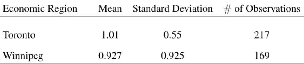
Next, we want to see how much variation we have across different country of birth groups within an economic region. We plot summary statistics for the gender ratio across different country of birth groups within the economic region of Toronto in 2005 (first row) and of Winnipeg in 2005 (second row). Table 2 shows there is quite a lot of variation across country of birth groups. In the case of Toronto, the average gender ratio is of 101 women per 100 men and the standard deviation is of 55 women per 100 men. The number of observations in the first row is the number of country of birth groups in Toronto in 2005. In the case of Winnipeg, the average gender ratio is 92.7 women per 100 men and the standard deviation is of 92.5 women per 100 men. The number of observations in the second row is the number of country of birth groups in Winnipeg in 2005.
Table 2: Summary Statistics for Gender Ratio across Immigrant groups for 2005 in Toronto and Winnipeg
Economic Region Mean Standard Deviation # of Observations
Toronto 1.01 0.55 217
Winnipeg 0.927 0.925 169
Notes: Summary Statistics for Gender Ratio across Country of Birth groups for 2005 in Toronto and for 2005 in Winnipeg. Each observation is a country of birth group in Toronto in 2005 (first row) or a country of birth group in Winnipeg in 2005 (second row).
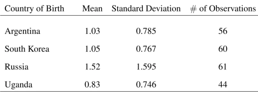
Next, we plot summary statistics for the gender ratio across different economic regions for a given country of birth in 2005. Table 3 below plots the summary statistics for the gender ratio across economic regions for the Argetina born popula-tion (first row), South Korea born populapopula-tion (second row), Russia born populapopula-tion (third row) and Uganda born population (fourth row).20 In the first row we see that, for the Argentina born population, the average gender ratio is 103 women per 100 men and the standard deviation is 78 women per 100 men. In the second row we see that, for the South Korea born population, the average gender ratio is 105 women per 100 men and the standard deviation is 77 women per 100 men. The third row shows that, for the Russia born population, the average gender ratio is 152 women per 100 men and the standard deviation is 159 women per 100 men. Finally, in the fourth row, the Table shows that for the Uganda born population the average gender ratio is 83 women per 100 men and the standard deviation is 75 women per 100 men. The number of observations in each row represents the number of economic regions in 2005 for which there were people of that country of birth. Hence, each observation represents an economic region in 2005.
Table 3: Summary Statistics for Gender Ratio across Economic Regions for given Country of Birth in 2005
Country of Birth Mean Standard Deviation # of Observations
Argentina 1.03 0.785 56
South Korea 1.05 0.767 60
Russia 1.52 1.595 61
Uganda 0.83 0.746 44
Notes: Summary Statistics for Gender Ratio across Economic Regions in 2005 for Argentina born population (first row), for South Korea born population (second row), for Russia born population (third row), for Uganda born population (fourth row). Number of observations in each row represent the number of economic re-gions in 2005 that had the given country of birth.
20These are just some examples since it would be too much to present information for all countries
of birth. Since we have the full universe of Canada, in our data we have information for all countries of birth and all economic regions.
Like previously mentioned one concern is that most businesses are started jointly by spouses something that is absent in our model. Looking in our data we find that only 29% of new firms started are started by both spouses. Furthermore, as explained previously in our main specifications we verify our results remain un-changed once we proceed to excluding these joint ventures.
Another possible concern is if spouses substitute from working for another firm to working for the firm started by their partner. In this case, we might wrongly interpret a positive impact of marriage on entrepreneurship as due to insurance when instead it is due to spouses working for their partner. In the data, we find that only 16.26% of new entries into entrepreneurship are accompanied by the spouse being reported as employee of the business. Furthermore, we also verify our main specifications are robust to excluding the subset of businesses for which the spouse works for the new firm started by their partner.
One possible concern with our identification strategy is the potential lack of ho-mophily in marriage in Canada. In particular, we might be worried that due to the high level of immigration from all around the world most couples are composed of two individuals born in different countries. A recent brief by Statistics Canada for 201121shows that of all couples in Canada : 66.9% are between two Canadian born,
18.2%are between two immigrants born in the same country, 3.7% are between two
immigrants of different countries of origin and 11.2% between one Canadian born and one immigrant. It follows that 85% of couples were between individuals born in the same country. Among immigrant only couples, 83% of couples were between individuals born in the same country. This highlights how despite the high immi-grantion rates to Canada, homophily is still relatively high in the population. This degree of homophily is also observed in other dimensions. The same brief reports that 87.6% of couples have one or more common mother tongues. Similarly, 90.2% of couples are composed of either two individuals that share the same religious affiliation or two individuals with no religious affiliation.
Finally, we might be worried that some of the variation in the gender ratio in our data comes from small populations of individuals of a particular country in a given economic region. In the robustness section we show our results are robust to
restricting the sample to cells with a minimum of men and women. 3.1.1 Results
In this section we present the main results of our specifications. We also include as additional controls : year dummies, changes in the share of total employment in the
oil, gas and mining sector, Shareoil
c,t, changes in the share of total employment in
the manufacturing sector, Sharemanuf
c,t , changes in the share of total employment
in the service sector, Shareserv
c,t , and changes in the share of population in differ-ent age groups for each economic region, country of birth and year triplet. Results are robust to not including this extra set of controls.
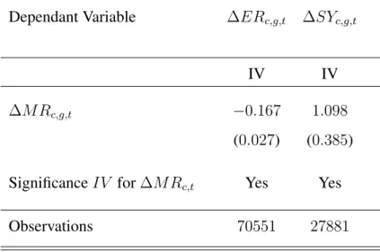
Column 1 of Table 4 presents the OLS results for our entry rate specification. We see that marriage rates are significant and positive if we don’t instrument for it. Column 2 shows that once we instrument for marriage rates, the coefficient flips sign and increases in magnitude. In particular, a 1 percentage point increase in the marriage rate is associated to a 0.2 percentage point drop in the entry rate into entrepreneurship. Given the 1% baseline entry rate in the data, this corresponds to a 20% drop in the entry rate into entrepreneurship. Finally, row 2 indicates that the instrument is significant at the first stage. Column 3 indicates the results are robust to including city dummies.
One concern with our results is that cultural determinants can be simulatenously determining the change in gender ratio and in entrepreneurship. To deal with this we can use the variation in changes in the gender ratio of a same immigrant group across two different locations. To do that we include country of origin dummies. Column 4 shows our results are robust to using this variation. First stage results for Table 4 can be found in Table 6 of the Appendix.
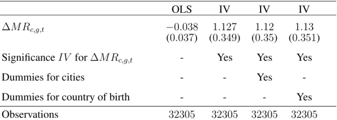
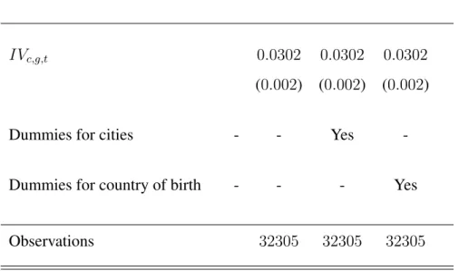
Next, we turn to the results on average number of employees of firms. Column 1of Table 5 indicates marriage, MRc,g,t, has a small negative insignificant effect on average size of firms if not instrumented for. Column 2 of Table 5 shows results for average size of firms once we instrument for marriage rates by our instrument, the gender ratio. Our estimate implies that a 1 percentage point increase in the marriage rate increases the average size by 1.13%. In other words, a 10 percentage point increase in the marriage rate increases average size of firms by 11.3%. Finally
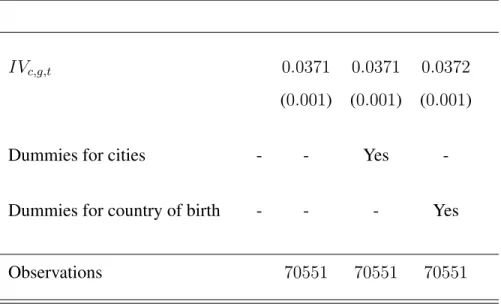
row 2 indicates that the instrument is significant at the first stage. Column 3 and 4 indicate that the results for average size are robust to the inclusion of city dummies or country of birth dummies. First stage results for Table 5 can be found in Table 7 of the Online Appendix.22
Note that when we include city dummies we are using variation in changes of the gender ratio across country of birth groups within a same city. In turn, when we include country of birth dummies we are using variation in changes of the gen-der ratio for a same immigrant group across different cities. Hence, these are two different sources of variation for which there is no reason ex-ante to expect similar results. Yet, despite this different source of varation, we get similar results in sign, significance and magnitude regardless of which of these two sources of variation we use. Furthermore, results for both entry and average size are robust in sign, mangnitude and significance to including dummies for each country of origin and year pair.23 Results are also robust to clustering at the economic region c level.
These results are consistent with the prediction of our model that the group (married vs unmarried) with the highest entry rate into entrepreneurship is also the one with the lower average firm size. Futhermore, note that this is true for both the OLS and IV specifications. Our results are consistent with the notion that the spousal insurance effect is dominated by the spousal sharing effect or by the negative effects on entrepreneurship of theoffspring effect.
The results are in line with married households being more selective in which business projects to implement. This implies that a decrease in marriage rates in-duces a fall in average productivity of the economy. In the next section, we look at this implication more formally.
22The number of observations for the average size regressions are smaller because for a country
of birth, economic region and year triplet to be included we need there to be entrepreneurs in that triplet. For the entry rate regression we just need there to be individuals in that country of birth, economic region and year triplet.
Table 4: Main specifications : Entry Rate Regressions
OLS IV IV IV
M Rc,g,t 0.0258 0.219 0.219 0.22
(0.004) (0.035) (0.035) (0.035)
Significance IV for MRc,t - Yes Yes Yes
Dummies for cities - - Yes
-Dummies for country of birth - - - Yes
Observations 70551 70551 70551 70551
Notes: Regressions of changes in the entry rate into entrepreneurship in economic region c, country of birth g and year t, ERc,g,t, on the change in the marriage rate in economic
region c, country of birth g, year t, MRc,g,t. Column 1 reports OLS results. Columns 2, 3
and 4 reports results when using our instrument. Our instrument is the change in the gender ratio. The gender ratio is defined as the total amount of women divided by total amount of men for that city c, group g, year t. Specifications include year dummies, changes in female labor force among married women, in average income among married men, in the share of population at each triplet (c, g, t) within 3 age groups, in the employment shares in oil and gas, manufacturing and services sectors. Standard errors are clustered at economic region c and country of birth g.
Table 5: Main specifications : Average Number of Employees Regressions
OLS IV IV IV
M Rc,g,t 0.038 1.127 1.12 1.13
(0.037) (0.349) (0.35) (0.351)
Significance IV for MRc,g,t - Yes Yes Yes
Dummies for cities - - Yes
-Dummies for country of birth - - - Yes
Observations 32305 32305 32305 32305
Notes: Regressions of changes in the log of average number of employees of firms in economic region c, country of birth g and year t, log(SY )c,g,t, on the change in the
marriage rate in economic region c, country of birth g, year t, MRc,g,t. Column 1 reports
OLS results. Columns 2, 3 and 4 reports results when using our instrument. Our instrument is the change in the gender ratio. The gender ratio is defined as the total amount of women divided by total amount of men for that city c, group g, year t. Specifications include year dummies, changes in female labor force among married women, in average income among married men, in the share of population at each triplet (c, g, t) within 3 age groups, in the employment shares in oil and gas, manufacturing and services sectors. Standard errors are clustered at the economic region c and country of birth g.
4 Implications for Average Firm Productivity
The results in the previous section make clear that higher marriage rates induce lower entry rates but larger firms on average. Through the lens of our model, the results indicate that higher marriage rates induce less firm creation but increase av-erage firm size and productivity. In this section, we use our results to discipline a back of the enveloppe bounding exercise of the implied change in average produc-tivity, E[z]. To do so, note that for all firms in the model we have
n(z, w) = (↵y✓ w ) 1 1 ↵e z 1 ↵. (52)
This in turn implies
E[n] = (↵
w)
1
1 ↵E[z] (53)
where E[z] is as defined in Equation 74 and E[n] is average number of employees. It follows that
log(E[z]) = log(E[n]) log(↵
w)
1
1 ↵. (54)
In the short and medium run we can argue w ⇡ 0 ) log(↵
w)
1
1 ↵ ⇡ 0. Hence,
log(E[z])⇡ log(E[n]). (55)
Given our estimates of the previous section it follows that a 1 percentage point increase in marriage rates is associated to 1.13% percent increase in average pro-ductivity. Of course, in the long run we expect wages, w, to adjust. If the main source of variation in (↵
w)
1
1 ↵ in the long run is the rise in wages, w, then our
es-timate of the impact of marriage on average firm productivity is a lower bound to the true long run effect. More generally, our estimate of the response of average size to marriage rates allows for us to calculate the implied changes in average firm productivity given any estimate of changes in wages.
5 Robustness Checks
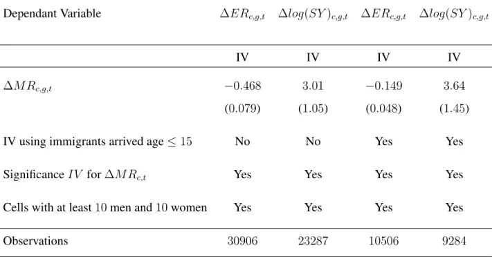
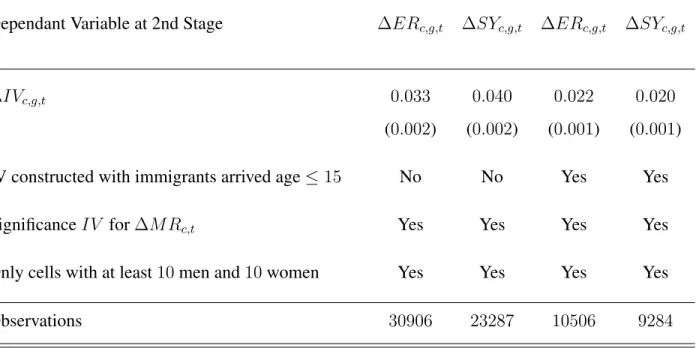
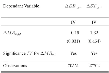
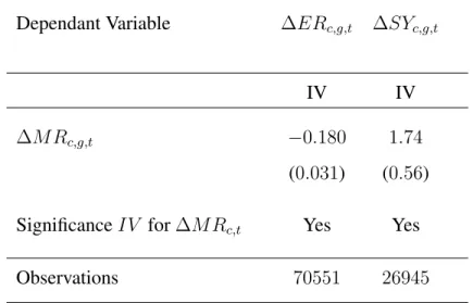
One concern with our strategy is that there might be economic regions with very low absolute numbers of individuals from a particular country. This would mean that a small arrival of individuals from that group produces large fluctuations in the gender ratio. To address this concern we verify our results are robust to restricting the use of economic region, country of birth and year triplets with at least 10 women and 10 men. Our results are unchanged in both sign and significance. In fact, the magnitudes actually increase. Results can be found in Columns 1 and 2 of Table 9 of the Online Appendix.
A second concern with our identification strategy is if there are city specific shocks yc,tthat are gender biased differentially across different immigrant groups. As such, men from particular immigrant groups could be more prone to move to particular cities relative to men of other immigrant groups. The result is that our instrument would be correlated to the error term. However, this is not a concern for individuals that arrived at an early age in Canada. As long as the choice of an immigrant of where to immigrate to in Canada is uncorrelated to the gender of their child, we can use these early age arrival immigrants to address this concern. Con-sistent with this argument, we verify our results are robust to using a gender ratio constructed using only individuals that arrived at age 15 or younger in Canada. Our results are unchanged in both sign and significance. For entry rates the magnitude is unchanged while for average size the effect is now stronger. Results can be found in Columns 3 and 4 of Table 9 in the Online Appendix.
6 Discussion on Alternative Mechanisms
The theoretical model is purposely tractable to keep the intuition clear and concise. However, there might be other economic mechanisms affecting entrepreneurship not present in the model.
Firstly, spouses might help individuals overcome borrowing constraints via wealth sharing or faster wealth accumulation. There are two ways borrowing constraints affects outcomes for an individual considering starting a firm. The first is that