HAL Id: hal-00617038
https://hal-mines-paristech.archives-ouvertes.fr/hal-00617038
Submitted on 26 Mar 2019
HAL is a multi-disciplinary open access
archive for the deposit and dissemination of
sci-entific research documents, whether they are
pub-lished or not. The documents may come from
teaching and research institutions in France or
abroad, or from public or private research centers.
L’archive ouverte pluridisciplinaire HAL, est
destinée au dépôt et à la diffusion de documents
scientifiques de niveau recherche, publiés ou non,
émanant des établissements d’enseignement et de
recherche français ou étrangers, des laboratoires
publics ou privés.
Experimental study and numerical simulation of the
injection stretch/blow molding process
Fabrice Schmidt, Jean-François Agassant, Michel Bellet
To cite this version:
Fabrice Schmidt, Jean-François Agassant, Michel Bellet. Experimental study and numerical simulation
of the injection stretch/blow molding process. Polymer Engineering and Science, Wiley-Blackwell,
1998, 38 (9), p.1399-1412. �10.1002/pen.10310�. �hal-00617038�
Expe
r
i
me nta
I Study
and
Nu
m e rica
I Si
m u
la
t
io
n
of
the Injection Stretch/Blow Molding Process
F. M. SCHMIDT,'**J.
F.
AGASSANT,2d M .
BELLET2'Ecole des
Mines d'Albi-CarmauxCampus
JarlardRoute de
Teillet81 01
3
AlbiCT
Cedex
09, France2Ecole
des M i n e s
de Paris
06904 Sophia-Antipolis, FhneeCEMEF-URA
CNRS
rz~. 1374The injection stretch/blow molding process of PET bottles is a complex process,
in which the performance of the bottles depends on various processing parameters. Experimental work has been conducted on a properly instrumented stretch/blow molding machine in order to characterize these processing parameters. The objec- tive being a better understanding of the pressure evolution, preform free inflation has been processed and compared with a simple thermodynamic model. In addi- tion, a numerical model for the thermomechanical simulation of the stretch/blow molding process has been developed. At each time step, mechanical and tempera- ture 'oalance equations are solved separately on the current deformed c o n f i g u ~ - tion. Then, the geometry is updated. The dynamic equilibrium and the Oldroyd B constitutive equations are solved separately using an iterative procedure based on
a fixed-point method. The heat transfer equation is discretized using the Galerkin methlDd and approximated by a Crank-Nicholson's scheme over the time increment. Succc:ssful free blowing simulations as well as stretchjblow molding simulations have been performed and compared with experiments.
1) InfTRODUCTION 1.1) Presentation of the Study
he injection strt:tch/blow molding process of
T
poly(ethy1ene terephtalate) bottles is a three step process (as sketched inm.
1): first the PET resin is injected in a tube-shaped preform [ 11, then this amor- phous preform is heated above the glass transition temperature[Z]
and h-ansferred inside a mold. Finally the preform is inflated with stretch rod assistance inorder to obtain the desired bottle shape [3].
The performance of PET bottles produced by this process depends on three main processing variables: the initial preform shape, the initial preform tempera- ture, and the balance between stretching and blowing rates. These parameters will induce the thickness dis- tribution of the bottle as well as the b i d orientation and crystallinity, which in turn governs the trans- parency and the mechanical properties of the bottle.
This article will deal only with the last step of the
*Corresponding author.
process, namely the stretching and blowing phase. Our objective is to propose a general thermomechani- cal approach that is able to take into account vis-
coelastic constitutive equations for PET as well as
complex boundary conditions. A two-dimensional vo- lumic finite element method h a s been developed, which is able to capture the shearing effects especially
at the contact zone between the moving stretching rod
and the preform. Numerical results have been com- pared with experiments performed on an instrument- ed stretch/blow molding machine. This model will be a useful tool in order to optimize the processing para- meters in order to obtain controlled thickness distrib- ution as well as final stress distribution.
1.2) Literature on Blow Molding Roceu
A few models have been developed [ 1, 2) in order to represent heat transfer inside a n infrared oven, but because of the complexity of the radiative transfer in a
transparent parison, the problem still remains open.
A few experimental works refer to the experimental in- vestigation of the kinematics of parison inflation. In several papers (3-6). the authors have recorded the
F. M . Schmidt, J . F. Agassant, and M. BeUet
RECIPROCATING SCREW
n
MOLD CLOSED
Rg. 1. Description of the injection stretch/blow molding process.
inflation of free (or confined) parisons using high speed video camera. In the case of confined parison inflation, they have designed transparent molds. These works represent an important contribution to the analysis of parison inflation, but the technique
still remains limited to simple mold geometries
(high
curvatures enhance visual distorsions). Experimental work close to the stretch/blow molding process has been performed on a well instrumented machine at
Corpoplast company (7): the preform inflation has been investigated using displacement sensors that are located inside the mold, but the force exerted by the polymer on the stretch rod has not been measured.
Finite element numerical simulations of the blow or stretch/blow molding step have been extensively de- veloped during the last decade. Most of the models as-
sume a
thin
shell description of the parison. Warby and Whiteman (8) as well as Nied et aL (9) proposed isothermal finite element calculations. These models, first developed for the thermoforming process. have now been applied to blow molding process. The rheo- logical behavior is approached by a nonlinear-elastic constitutive equation issued from the rubber-like ma-terials theory. Kouba et
aL
(10) extended the previous model to a viscoelastic fluid (KF3KZ constitutive equa- tion). Several models use a volumic finite element ap--
MOLD CLOSED
MOLD OPEN
-
PART EJECTU
1 1
EJECT
proach. In 1986, Cesar de Sa (1 1) simulated the blow- ing process of glass parisons assuming an Arrhenius temperature dependent Newtonian behavior. Chung (12) carried out simulations of the
PET
stretch/blow molding process using the AE3AQUS@ s o h a r e . The model assumes the elasto-visco-plastic behavior and thermal effects are neglected. Poslinski et aL (13) in-troduced nonisothermal effects in a simplified geome-
try. In order to take into account the phase change, the latent heat of solidification was included in the heat capacity of the material. Debbaut et aL (14) also
performed nonisothermal viscoelastic blow molding simulations with a Giesekus constitutive equation, but they presented numerical results only in the case of a Newtonian fluid.
In conclusion, the thin shell assumption, which permits 3D finite element computations, is often used and commonly associated to the hyperelastic behavior issued from solid elastic media. The finite element vo- lumic approach issued from the blow molding of glass
parisons is generally employed with liquid-We consti- tutive equations (Newtonian, viscoelastic) and is limit-
ed to 2D computations. In the stretch/blow molding step, the contact between the stretch rod and the bot- tom of the preform induces shear deformations as well as high and localized temperature gradients,
Stretching stage
which actually just.@, a volumic approach in order to obtain an accurate description of the deformation.
v, (mm/s) 500
2) EXPERIMENTAL
INVESTIGATIONS
2.1) I n w e n t a d :Mold of a StretchlBlow Molding Machine
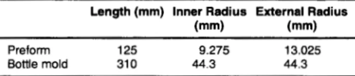
Experiments were performed on a well-instrument- ed mold at the Side1 Company (1 5). The dimensions of the preform and of the mold are summarized in Table
1. The instrumentaticln is described in Fig. 2 the dis- placement of the stretch rod is controlled and the force exerted on the stretch rod is recorded versus time using a force sensor. The blowing pressure is
recorded versus timc: using a pressure sensor (the pressure value is actiially different from the imposed blowing pressure). Nine contact sensors at the mold wall permit to identify the contact time between the polymer and the mold.
The parameters asslxiated with the stretching stage are the velocity of the stretch rod u,, which is applied until the preform contacts the bottom of the mold, and the preblowing step (Rps = displacement of the stretch rod before the, inflation pressure is imposed). The parameters associated with the inflation stage are
Pps, the maximum pre-blowing pressure (low-pres- sure) imposed during a preblowing time Dps for initi- ating the general shape of the bottle, and Ps, the m a - imum blowing pressure (high-pressure) that is applied during a blowing time D s in order to flatten the poly-
Preblowing stage
Table 1. Dimensions of the Bottle Mold and the Preform. Length (mm) Inner Radius External Radius
(mm) (mm)
Preform 125 9.275 13.025
Bottle mold 31 0 44.3 44.3
p, (Pa) 5 x
lo5
Dps (s) 0.3
mer along the mold wall. The preblowing air-rate Qps and the blowing air-rate Qs are prescribed by the op- erator but not measured.
Qpical values of the process parameters of the stretch/blow molding step are referred in Table 2. The
I
R,, (mm) 1 Blowing stageI
D, (s) 1.5 force sensor preform pressure contact senbor5 sensorFlg. 2. Description of the <mnstrumented mold of a stretch/blow
molding machine.
t
0 0.1 0.2 0.3 0 . 4 0.5 0 . 6 0 . 7
t ( s ) pre
-
blowing stageQ. 3. History of pressure uersus time.
F. M.
Schmidt, J. F. Agassant, andM.
Belletpressure is measured directly in the preform (see Flg.
3). In addition, short-shot bottles produced for the target process are time-located on the recorded pres- sure curve.
As shown in Fig. 4, the measured stretching force of the rod versus time starts from zero (or from a very
450 400 350 300
5
.-
250-
Y2
200 150 100 50 0 Rps = 40 mm -+--- 0 0.05 0.1 0.15 0.2 0.25 0.3 0.35 0.4 tb)Flg. 4. M e a s u r e d siretching force of the rod versus time.
Flg. 5. Location of the contacts sensors on the mold waU
low value), and then the curve rises to a maximum and decreases continuously. Note that when Rps in- creases, the maximum of the curve increases. In pre- vious papers (16. 13, we pointed out that the increas-
ing
part and the decreasing part of this curve may be related respectively to elastic and viscous phenomena. The location of the contact sensors (from no 1 to no 9) on the mold wall is indicated in FXg. 5. Recorded contact times versus the location of contact sensors are plotted in Flg. 6 using the process parameters that are referred inTable
2. When the preblowing delayRps is increased from 1 mm to 40 mm, all the contact times between the polymer and the mold increase and
the contact times are more homogenous in the central part of the bottle. In addition, if we plot the measured thickness distribution versus longitudinal coordinate
at the end of the process for the two values of Rps (see
Fig. 7). we note that an increase in the preblowing
0.55 1 I I I 1 I I I I 0.5
p
,
R p s = l m m -+-- Rps = 40 mm - + - - - 0.25'
I I 1 I I I I 1 2 3 4 5 6 7 8 9no sensor contact
--.-.1 I--_.m.
6. Contact times uersus nurnber of contact sensors.I I I I
0.31 0.32
I
Fg. 8. Diflerential pressure us.
time.
0 1
delay induces more material displacement from the neck to the bottom of the bottle.
2.2) Mecutuement and Calculation of the h t e l n a l Reuolre
In fact, in industrial blowing tools, the inflation pressure is only imposed and measured in the blow- ing device upstream and not inside the preform; sig- nificant differences may be observed between these
two pressures. Let us consider now the free inflation of a preform. The preform is heated in a silicone oil bath in order to obtain a uniform temperature distrib- ution (T = 95"C, 100°C. 105°C). A "nominal" pressure has been imposed to a constant value of 0.27 MPa in
the upstream blowing device for each case and the differential inflation pressure Ap,
( t )
= pa ( t )-
po (pa( t )
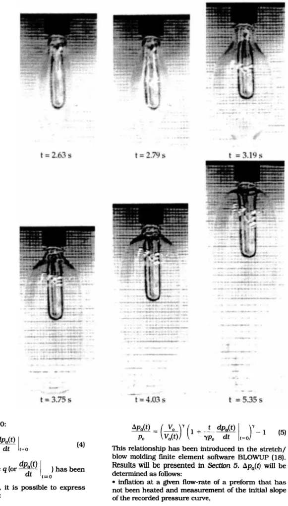
inflation pressure, po atmospheric pressure at ambi- ent temperature) is recorded versus time using a pres- sure sensor (see Fig. 8). For each temperature, free in- flations were recorded using video camera. In Fig. 9, successive preforms duing free inflation are presented at T = 105°C. Three different parts may be observed
on each curve:
a first part where the pressure rises to a maximum (less than 0.3 ma), during which the polymer is not inflated (the internal volume of the preform remains constant);
a second part where the pressure decreases contin- uously to a minimum because the volume increases:
the last part of the curve where the pressure in-
creases again because of the "strain-hardening" of the material, which is in fact related to the development of crystallinity under biaxhl stretching.
It is to be noted that the duration of these three steps during free inflation is strongly dependent on temperature. This experiment demonstrates that the evolution of the intema pressure and the inflation of the preform are highly coupled. It is also to be noted that the recorded internal pressure is significantly dif-
2 3 5 6 7 9 10
time
(s)
ferent from the "nominal" pressure. In order to better understand this pressure evolution, we develop here- after a simple thermodynamic model. As sketched in
Fig. 10, we consider that air flows in the "control vol- ume" V,(t) at an air-rate q with a velocity field, pres- sure pe and a temperature T,. We assume that the air- rate q is constant during the pre-blowing stage, which results in the following relationship between the air
mass
&(t)
(occupying the volume V,(t)) and q:dm,
q = __ = cte
+
m,(t) = m,+
qtdt
where m, is the air mass within the parison at time
t = 0. Using the following assumptions:
no heat transfer between the air volume and the surrounding medium,
air is an ideal
gas,
the global energy balance during the time step dt over the volume Va( t) may be simplified as (1 8):
d d Te
dt dt 'a
-- (Ln(p,VY,)) = - (Ln(rnY,)) - -
where y = 1.4 for air. In order to obtain a simplified re- lationship, we assume T,
=
T,, which is consistent with the assumption of no heat transfer with the sur- rounding medium. Using E q 1 a n d ma = pa V,,Equation 2 reduces to:
(3)
where po is the air specific mass at time t = 0 (initial ambient temperature). Knowing the volume VJt) (due to parison inflation), this relation should provide the pressure value p,(t). However, the experimental deter- mination of the air-rate q is very difficult. In order to overcome this difficulty, we suggest that q should be determined through a n inflation test at constant vol- ume V, (for example, using a prefonn which has not been heated). Differentiating Eq 3 with respect to time,
1403
F. M . Schmidt, J. F. Agassant, and M. BeUet
Fig. 9. Preformfree i n j h b n fl= 105°C).
t =
3 . E s
w e obtain at initial time t = 0:
t
=
4.03
5t
=
5.35
5(4) This relationship has been introduced in the stretch/ blow molding finite element software BLOWUP (18).
Results
will
be
presented
in Section
5. Ap,(t) will be determined as follows:Once the specific flow-rate q (or Q
dpdt’s
It
=/
has been .-a inflation at a given flow-rate of a preform that has
not been heated and measurement of the initial slope of the recorded pressure curve,
POLYMER ENGINEERING AND SCENCE, SEPlEWER l a , Vol. 38, No. 9 experimentally determined, it is possible to express
the idlation pressure Ap,(t): 1404
calculation of the initial internal volume of the pre- computation of tht: internal volume of the preform VJt) at each time step,
determination of Apa(t) using Eq 5.
form
v,,
3)
BOUNDARY
CONDITIONSThe boundary conditions are presented in Fig. 1 1 :
along the contact surface between the rod and the preform
u = u, (sticking contact)
T
= T, (prescribed temperature at the rod: note that the temperature of the rod is not easy to measure) along the internal mrface of the preform, which isnot in contact with the rod
(U
. n')
.n'
= - Ap,(t)( k V T )
. n'=
-
&(T-- T,)where
h,
is the heat transfer coefficient between the polymer and the air inside the parison; however, the extracted heat flux car^ be generally neglected.along the external surface of the preform, which is in contact with the mold
v = o
T = T, (prescribed temperature of the mold) along the external surface of the preform, which is not in contact with the mold
(g .
n')
' r; = 0( k V T ) .
n'=
- h,(T- T,)where
h,
is the heat transfer coefficient with the mold, which will vary continuously during the infla- tion process.-n
4) NUMERICAL RESOLUTION 4.1) Thermomechpnlcal Equations
The numerical simulation of the stretch/blow mold-
ing
of an incompressible viscoelastic fluid (Oldroyd B type) consists in solving the following set of equations on the domain R occupied by the preform:where g = - p ' i
+
2rlsi+
7 (6)p(7-G) = V
.
v . r ; ' = o
(7)I
with the above-mentioned boundary conditions. In this model, the mechanical equations (Eqs 6 to 8) and the temperature balance equation (Eq 9) are solved separately on the deformed configuration R" at cur- rent time step
t,,
(see%.
12). The current values ofthe velocity vector
i?',
the pressure p'" and the extra- stress tensor 7" are determined first. Then the tem- perature field?'
+ is computed. Finally, the geome-try is updated from R" to R" + using the 2nd order
explicit Euler rule:
Rg. 10. Volumefree blowing at a constantjlow rate.
RADIAL SYMMFTRY
;j
I AXIAL +I I I I I I I SYMMEfRY; \
BOTTLE- - -
PREFORM Rg. 1 1 . Boundary conditions. MOLD/-
F.
M.
Schmidt, J. F. Agassant, and M. BeUet 4.2) Remolution of the M a c h a n i d Equation8The resolution method is summarized hereafter. Full details about the numerical algorithms are given elsewhere (16, 17).
4.2.1) Splitting Technique
At each time step, an iterative procedure based on a
fixed-point method is used in order to solve EQuations 6 to 8. The first sub-problem, called the "Generalized Stokes Problem" (GSP), deals with an incompressible Newtonian fluid flow, perturbed by a known extra- stress tensor 1 computed at the previous fixed-point iteration
(k-u
(Equations 6 and 7 ) . The second sub- problem consists in determining the components of the extra-stress tensor 1 for a known velocity field by solving the time-discrekd constitutive equation (Eq8). The procedure is repeated until convergence.
4.2.2) Spatial Discretization
The domain Q is approximated by a set of 6-node
n = l
t n
= O
m
I
I
isoparametric triangles
Th
(quadratic element, seem.
13), which are deflned by the shape functions $k. The nodal velocity field is expressed in term of the compo- nent u k of the nodal velocity vectors with the same shape functions. The pressure is constant by element.
Using the Galerkin method, the discretized equations of GSP at current time
t,
lead to the following system:+ - + +
where the matrix A,
B
and the v y t o p V, P, F are given elsewhere (16). In order to find V,P. we use an itera- tive scheme derived from Uzawa's algorithm (1 6). Thebounded set of linear algebraic equations is solved by
a direct Crout decomposition.
4.2.3) Viscoelastic Equation
As the different integrals in Equation 1 1 are evaluat- ed by the Gauss-Legendre point integration rule, the components of the current extra-stress tensor
xn
are needed only at the Gaussian points of each element. Consequently, the tensorial equation (Eq 8) is solvedat a local level; it reduces to a (4 x 4) linear algebraic system.
where the matrix
K,
and the vectors2u,
2"
are defined elsewhere (18). The set of linear algebraic equations (Eq 13) is solved by a direct Gauss method.4.3) Thermal Bplpnce Equation
The time differential equation (Eq 9) is approximat- ed by a Crank-Nicholson's scheme over the time in-
t n + l =
tn
+
Atn+l
n = n + l
-
Igeometry
f
Constant pressure 0 Velocity, TemperatureI
Flg. 13. Mesh of the preform and P2-PO element
crement At,,. Using Galerkin method, the discretized equation (Eq 9) at current time t,, leads to the follow-
ing
system:$ " A I -
$"
$n+1 +5ll
~C*( A~ ) + K * / - ) i S * = O (14) The capacity+Tatrix C:, the conductivity matrix
K,
and the vectors T. S are defrned below:4
+ JakV Y k V
9,dv1
S , = - l n h a T a . Y l d S - h , T ; V r , d s + I W V r , d v nEach matrix M x (= C*, K*, $) takes the following form: (15)
3 1
2 2
which results from a linearized technique (19) in order to avoid an iterative resolution of Eq 14. Only the non-
reversible part of the strtss tensor
4"
(viscous part) con-tributes to the dissipated energy W.
1r.
M* ~ ~- M K - ~ n - 1
W = T i v : = 2(qs
+
q,)b : E = 2q :t
'.
=0.65sFlg. 14. Intermediate 1)ubble shapes (T = 105°C).
Table 3. Processing and Rheological Parameters for Free Inflation at T = 105°C.
Process Parameters Rheological Parameters
(bars) (MPals) 2.58
The linear system (Eq 14) is solved by a direct Crout decomposition.
4.4) Variation of Viscosity With Temperature
T h e empirical relation proposed by Ferry et aL (20)
accounts for rapid variation of the viscosity between the glass transition Tg and Tg
+
100°C.- C : ( T - ;)
where '2: = 8.38 R' and C z = 42.39
K
(21).t = 0.27s
u
t =1.5sRg. 15. Intmmedmk ' bubble shapes (T = 105"C, 8, = 125%). 1407 POLYMER ENGINEERING AND SCIENCE, SEPTEMBER 1998, Vol. 38, No. 9
F.
M.
Schmidt, J.F.
Agassant, andM.
Bellet0,3
-
0.25
z
z
g0‘2
2
5
0,15
2
0.1
g0.05
6
0
L-
m _C___--r--r--- Computed-
Measured----.
-
Computed-
Measured---
Q. 16. Diimeniial injlation pressure u e r s ~ l s time.
6 )
APPLICATIONS
6.1) PratarmFreebnption
Let us proceed to free inflation simulations at T =
105°C in order to compare the computed differential inflation pressure to the measured one (see Seetion 2.2). Processing parameters are given in Table 3. Viscoelastic parameters have been adjusted in order to obtain the same maximum pressure. We assume that the relaxation time remains constant. It appears immediately in R g . 14 that the expansion of the pre-
form and especially the radial expansion is unlimited. This problem, which is not observed experimentally, occurs because the strain-hardening phenomenon of the material, related to the development of crystallini- ty under biaxial stretching, is not taken into account in the numerical model, and this problem has not
Flg. 17. Intermediate bottle shapes.
n
t = O s
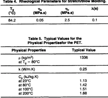
Table 4. Rheological Parameters for StretchiBlow Molding.
84.2 0.05 2.5 0.1
Table 5. Typical Values for the Physical Propefliesfor the PET. Physical Propsrties Typical Value
1336 0.25
cp
(kJ/kg.K) at 23°C at 80°C at 100°C at 200°C 1.13 1.42 1.51 1.88been addressed in this paper. Introducing a viscosity dependent on the generalized strain E =
,
b
d
z
asproposed by GSell(22):
t
strain - hardeningtm
where
Eo
is a reference value, leads to limit the expan- sion of the preform (see Fig. 15). In that case, the computed differential inflation pressure and the mea- sured one are plotted in Fig. 16. We note that the agreement is fair between the two curves except in thet=0.36s
t=
0.4
s
t=
0.45
s
last part. The computed preform inflation remains, however, significantly different from the free inflation that has been recorded using video camera (&. 9).
5.2) S e t m p of a Real Stretch/Blow Molding
R0CG.I)
We study now a s tretch/blow molding operation. The geometries of the bottle mold and of the preform, the processing parameters have been previously refer- enced in FQ. 5, Table 1, and Table 2, respectively (see
Section 2.1). The initial mesh of the preform has
been shown in Fig. j 3 . For this thermomechanical
simulation, we use the experimental pressure that has been plotted in Fig. 3 (i.e. the pressure is not cal- culated using Eq 5). The viscoelastic rheologid para- meters (Table 4) have been determined by
fitting
on the traction force of an amorphous PET sample, in- jected in the same conditions as the tube shaped pre-500
7
I I I I 1 Non-isothermal- Isothermal - - - -. experimental~-
,_---___ 350form (18). Typical values for the physical properties of the PET are referenced in Table 5. The value of the heat transfer coefficient between the air and the poly- mer is considered to be
!-+,
= 10 W/K.m2. A high value for the heat transfer coefficient between the mold and the polymer h,,, = 500 W/K.m2 has been applied at the interface between the preform and the mold after con- tact. The initial temperature of the preform is 100°C. Besides, it should be noted that the internal and the0 0.05 0.1 0.15 0.2 0.25 0.3 0.35
tb)
Hg. 18. Measured a m ! computed siretch rod us. time.
h E E v 3 2.5 2 1.5 1 0.5 0 non-isothernial - isotherm31 dz ta - i- - -
1
non-isothernial , h t i herma1 - experimental dz ta - i- - - I I I I I I I I \ \ __---_--_
' - - - , , - 4 : - - - - . ~ - - - , --- I I I I 0 50 100 150 200 250 300 350 w-1 I - - -Flg. 20. Temperature distribution at the end ofthe process.
\-
3
Fig. 19. Thickness distrihution at the end of the process.
F. M . Schmidt, J . F. Agassant, and
M.
Bellet. A
- B
external heat transfer coefficients are assumed to be the same.
lplsure 17 presents intermediate bottle shapes from the beginning to the end of the process. The computed isothermal and nonisothermal stretching force exerted on the stretch rod vs. time are quite equivalent (see
Rg. 18). This result was expected because heat trans-
fer becomes important only when the outer surface of the preform reaches the inner surface of the mold and on a small area of the bottom of the preform that is in
contact with the rod. The nonisothermal stretching force is lower than the isothermal one. This is due to
F@. 21. Temperature distribution along material lines.
h
u
K
110
100
9080
70
60 50 4030
L
" II
I 1 I II
0 0.2 0.40.6
0.8
1?-
Inner surface
(b>
?-
Outer surface
Fg. 22. Comparison of the contact times. 0.5 0.48 0.46 0.44 0.42 Y 0.4 0.38 0.36 0.34 0.32 0.3 0.28 h
Inner surface
Outer surface
1 2 3 4 5
6
7 89
No Capt.
T
1'
the dissipation energy related to high deformations, which increases the temperature locally. The compari- son between the computed thickness distribution and the experimental data at the end of the process is shown in Flg. 19. The agreement is better with a non- isothermal model than with an isothermal one.
The temperature di:jtribution at the end of the pro- cess is represented i n Fig. 20 at different locations (bottom of the bottle, details of the mold, neck of the bottle). The contact between the stretch rod and the bottom of the preform as well as the contact between the bottle mold and the outer surface of the preform induces high temperature gradients throughout the thickness (maximum 50°C), which just@ the volumic approach in order to obtain an accurate description of the temperature distribution. More enlightening is to plot the temperature distribution along three material lines, which are located, respectively, at the neck of the preform (yA = 290 mm), at the center of the pre- form (y, = 250 mm), and at the bottom of the preform
(x, = 6.9 mm) (see F'ig. 214. For each material line, the temperature distribution is represented vs. the nondimensional cumlinear coordinate s in the thick- ness direction (Rg. 21 b). We note that the temperature increases from the upper material line (A) to the lower one (C). This is due 1.0 the expansion of the preform, which occurs from the neck to the bottom of the bot- tle. So, the contact between the preform and the mold occurs later for line C than for line A. More interesting is that the temperature distribution along line C at the end of the process is partly higher than the initial temperature (see dashed line), which is related to the energy dissipation during inflation. This phenomenon has been observed experimentally.
Contact times versus location of contact sensors for
the isothermal model are plotted in Flg. 22 and com- pared with experiments. Contact times computed using Oldroyd B model are closer
than
the Newtonian one. Consequently, it appears that the kinetic of con-tact (and consequently the kinetic of blowing) depends on the rheological behavior.
6) CONCLUSION
Experiments have been conducted on a well-instru- mented stretch blow molding machine: stretching forces as well as contact times between the polymer and the mold have been recorded. The bottle thick- ness distribution has been measured for various pro-
cessing
parameters.A coupled model for the thermodynamic of the air
and for the thermomechanical idation of the parison has been proposed. A finite element model and a vis-
coelastic differential constitutive equation have been used. Viscous dissipation, as well as the temperature gradient between the mold and the molten polymer, has been considered. The comparison between experi- mental and numerical rod stretching forces is fair.
The discrepancy is more important when considering the thickness distribution and the contact kinetic.
Further developments will necessitate a better un- derstanding of the rheology of PET during the stretch blow molding operation (amorphous, i.e., liquid at the
beginning of the process, and semicrystalline, i.e., solid at the end of the process).
ACKNOWLEDGMENT
This research was supported by Side1 Company and the Rench 'Ministere de la recherche" (MHT no 9OA
136).
CP
Fh
9'
h,
Ik
- -r'
1 - 3i
= -(Vu = 2 *kr
RF. M.
Schmidt, J.F.
NOMENCLATURE heat capacity gravityheat transfer coefficient between air and polymer
heat transfer coefficient between mold/ stretch rod and polymer
identity tensor heat conductivity
unit outward n o d vector number of nodes
arbitrary pressure velocity field
discrete velocity field
assembly of the nodal velocity components assembly of the nodal pressure vector assembly of the nodal applied forces time
temperature field
assembly of the nodal temperature field temperature of the mold
temperature of the air
coordinate vector
discrete coordinate vector coordinate vector at time I?,,
+
(tf.V)[.] - VZ.[.] - [.].'VGupper convective time derivative acceleration field
+
'VV')rate of strain tensor associated with total viscosity
viscous part of the total viscosity viscoelastic part of the total viscosity viscosity at glass transition temperature relaxation time
specific mass
specific mass at glass transition temperature Cauchy stress tensor
extra-stress tensor shape functions
boundary of the domain R
part of the boundary
r
that is not in con- tact with the rodpart of the boundary
r
that is not in contact with the molddomain occupied by the preform
Agassant, and
M.
BelletREFEREMCES 1. P. Lebaudy, Polymer, 39, 1887 (1992).
2. M. D. Shelby, SPE ANTEC Tech. Papers, 8 7 , 1420 3. M. R. Kamal. V. Tan, and D. M. Kalyon, Polgm Eng. 4. M. E. Ryan and A. Dutta, Polyrn. Eng. Sci, 22, 569 5. A. Dutta and M. E. Ryan, Polyrn Eng. S d , 24, 1232
6. W. P. Haessly and M. E. Ryan, Polyym Eng. S c i , 88, 1279 (1993).
7. M. Cakmak and J. L. White, J. AppL Polyrn Sc., S O ,
3679 (1985).
8. M. K. Warby and J. R. Whiteman. Comp. M e t h AppL
M e c h Engng., 68, 33 (1988).
9. H. F. Nied. A. Taylor, and H. G. D e Lorenzi, Polyrn Eng. Sci, SO, 1314 (1990).
10. K. Kouba a n d J . Vlachopoulos, 'Modeling of Thermoforming and Blow Molding," Theoretical a n d Applied Rheology, Proc. XIth Congr. o n Rheology, Brussels, Belgium Wugust 17-21, 1992).
11. J. M. A. Cesar de Sa, Engng. Comp., Vol. 3, December 1986.
12. K. Chung, J. M a t Shap. Tech, 7 , N"4, 229 (1989). 13. A. J. Poslinski and J. A. Tsamopoulos, AIChE J., 36.
NO12 (December 1990).
14. B. Debbaut, B. Hocq, and J. M. Marchal, SPE AMEC Tech Papers, 39 (1993).
15. L. Thomas, "Vexiflcation experimentale d u n e these SIX
la modelisation d u soufflage avec bi-orientation de bouteilles en P.E.T.," (in French), Report, Ecole des mines de Douai (1991).
16. F. M. Schmidt, J. F. Agassant, M. Bellet, and G. Denis. "Numerical Simulation of Polyester Stretch/Blow Molding Process," Numiform 92, Roc. 4th Int. ConJ OR
Nwnerical Methods in Industrial Forming Processes, pp. 383-88. Balkema (September 1992).
17. F. M. Schmidt, J. F. Agassant, M. Bellet, a n d L. Desoutter, J. Non-Newt. Fluid M e c h , 64, 19 (1996). 18. F. M. Schmidt, J. F. Agassant. and M. Bellet, SPE
ANZECTech Papers, Is, 817 (1997).
19. M. Zlamal, 'Finite Element Methods for Non-Linear Parabolic Equations," R.A.I.R.O. Numerical analysis, Vol. 11, n"1, 93 (1977).
20. J. D. Ferry, Viscmlasiic properties of Polymers, 3nd Ed.,
J. Wiley. New York (1980).
21. G. Le Bourvellec, Thesis, in French, Universilk Pierre et Marie Curie, Paris VI (1984).
22. C. GSell, "Instabilites de deformation pendant l'etirage des polymeres solides," in French, Revue Phys. AppL,
28, 1085 (1988). ( 199 1). sci. 21, 338 (1981). ( 1982). (1984). Reoeived July 28, 1997 Revised November 1997
1412 POLYMER ENGINEERING AND SCIENCE, SEPTEMBER W&?, Vol. 38, No. 9
Powered by TCPDF (www.tcpdf.org) Powered by TCPDF (www.tcpdf.org) Powered by TCPDF (www.tcpdf.org) Powered by TCPDF (www.tcpdf.org) Powered by TCPDF (www.tcpdf.org) Powered by TCPDF (www.tcpdf.org) Powered by TCPDF (www.tcpdf.org) Powered by TCPDF (www.tcpdf.org) Powered by TCPDF (www.tcpdf.org) Powered by TCPDF (www.tcpdf.org) Powered by TCPDF (www.tcpdf.org) Powered by TCPDF (www.tcpdf.org) Powered by TCPDF (www.tcpdf.org) Powered by TCPDF (www.tcpdf.org)