HAL Id: hal-01599444
https://hal.archives-ouvertes.fr/hal-01599444
Submitted on 17 Oct 2017
HAL is a multi-disciplinary open access
archive for the deposit and dissemination of
sci-entific research documents, whether they are
pub-lished or not. The documents may come from
teaching and research institutions in France or
abroad, or from public or private research centers.
L’archive ouverte pluridisciplinaire HAL, est
destinée au dépôt et à la diffusion de documents
scientifiques de niveau recherche, publiés ou non,
émanant des établissements d’enseignement et de
recherche français ou étrangers, des laboratoires
publics ou privés.
Evaluation and design: a knowledge-based approach
Élise Vareilles, Michel Aldanondo, Paul Gaborit
To cite this version:
Élise Vareilles, Michel Aldanondo, Paul Gaborit. Evaluation and design: a knowledge-based approach.
International Journal of Computer Integrated Manufacturing, Taylor & Francis, 2007, 20 (7), p.
639-653. �10.1080/09511920701566517�. �hal-01599444�
Evaluation and design: a knowledge-based approach
E´. VAREILLES*, M. ALDANONDO and P. GABORIT
Centre de Ge´nie Industriel, E´cole des mines d’Albi-Carmaux, Campus Jarlard,
81013 Albi CT Cedex 09, France
The aim of this communication is to describe how aiding-design tools can evaluate designed solutions to help users make the best choices, avoid design mistakes and reduce the design time-cycle. First, we will compare the two main methods for aiding design— behaviour simulation tools and domain knowledge simulation tools—and look at their advantages and drawbacks. We will focus on tools based on knowledge because of their ‘interactivity’ and for their ability to represent domain knowledge and show how they can be extended to evaluate designed solutions. We will then concentrate on an aiding-design tool based on constraints and see how a solution can be evaluated using an evaluation function. As such a tool has already been developed as part of a European project to help metallurgists design and evaluate heat treatment operations, we end with the presentation of a real example.
Keywords: Evaluation of solutions; Interactive aiding design; Constraints; Application
1. Introduction
It is very important in aiding design to know the relevance of the solutions obtained. Indeed, it is necessary to know if one solution is better than another in order to make a good decision. An estimation of the relevance of the solutions is therefore essential. We mean by estimating a solution an evaluation of its quality, its performance and its efficiency. The question of the relevance of the solutions is even more crucial in the context of integrated design where designers come from different domains and have different (and, most of the time, conflicting) objectives (Huang 1996, Magrab 1997), e.g. the maximization of the performance and quality of a product and, simultaneously, the minimization of costs. The solution must, at best, respect the different objectives.
There are two main ways of helping users make choices by giving an idea of the behaviour of systems and characterizing the relevance of solutions: behaviour simulation, which is mainly based on mathematical expressions, and domain knowledge simulation, which is mainly based on ‘know-how’
and experimental knowledge. These two approaches can evaluate the relevance of a solution as follows.
. Behaviour simulations, for instance event-driven simulations (Banks et al. 1984), finite element models (Szabo and Babuska 1991), or models based on virtual reality, consider the evolution of a problem through time. They work well when problems have a temporal or physical behaviour that can be modelled by mathe-matical formulae. In general, the solutions returned by behaviour simulations are optimized following several criteria (Fu 2002) which lead to one of the optimal solutions; the relevance of the solutions is quantitative. The process of behaviour simulation can be divided into three steps. First, the user has to design his/her solution to the problem; secondly, (s)he has to simulate its behaviour; and, finally, (s)he has to decide if the solution is the relevant one or not. If not, (s)he has to re-design the problem and loops, as shown in the left part of figure 1. The aiding-design process is then a trial and error one.
. Domain knowledge simulations, for instance case-based reasoning (Riesback and Shank 1989), expert systems (Buchanan and Shortliffe 1984) and con-straint satisfaction problems (Montanari 1974), are mainly based on the ‘know-how’ of experts and provide experts’ advice. Experts’ know-how is domain knowledge, resulting from the experts’ skills and abilities. This kind of knowledge cannot be extracted and modelled easily. Usually, the solutions returned by domain knowledge simulation give approximate ideas of the result; the relevance of the solutions is qualitative. The process of using domain knowledge simulation can be divided into two steps: firstly, the user is guided step by step by the experts’ advice in order to design his/her problem and finally an approximate idea of the solution is found. Then the user has to decide if the solution is the relevant one or not. If not, (s)he has to re-design the problem by making different choices respecting the experts’ advice, as shown in the right side of figure 1. The aiding-design process is more an interactive one. Behaviour simulations are mainly used to optimize solutions, whereas domain knowledge simulations are mainly used to assist decisions in an interactive way. These two methods are not in conflict with each other and can be used to complement one another in different ways (Tsatsoulis 1990). For instance, and as shown in figure 1, the user can start with a domain knowledge simulation in order to design and estimate the solutions of her/his problem and then (s)he can use a behaviour simulation to obtain a more accurate result.
The aim of this paper is to show how the relevance of the solutions can be estimated or evaluated in domain knowl-edge simulations in order to help users make better decisions. We concentrate on the tools based on knowledge because of their ‘interactivity’ in aiding the design process and their ability to represent domain knowledge, and we study how they can be extended to evaluate the designed solutions. In section 2 we will look at different domain knowledge simul-ation tools and different methods of evaluating solutions. In section 3 we will concentrate on aiding-design tools based on constraints because of their consistent properties and see how a solution can be evaluated in such a case. Section 4 will illustrate our proposition with a real example.
2. Knowledge-based systems and evaluation functions There are several ways of modelling an expert’s knowledge to use it in aiding the design process. Experts’ know-how can either be implicitly expressed (embodied in past cases, for instance) or explicitly expressed (as mathematical expressions). Several methods of evaluating the relevance of solutions also exist and can be determined directly by experts or learned from past experiments. If the relevance of the solutions corresponds to a set of simple and independent data, it can be directly embodied in the system; if not, a method of evaluating the relevance of the solution must be added.
2.1. Implicit knowledge
In case-based reasoning (CBR) (Maher et al. 1995), expertise is embodied in a library of past cases, rather than Figure 1. Knowledge and simulation aiding-design tools.
being encoded in classical rules. Each case typically contains a description of the problem, plus a solution and/or the outcome. The knowledge and reasoning process used by experts to solve the problem is not recorded, but is implicit in the solution. In order to find a solution, the user describes her/his problem through a list of parameters and, after all the user’s inputs, the problem described is matched against the cases in the data base. A similarity function (Kolodner 1993) makes it possible to detect and classify similar cases and the most similar or the most adaptable ones are retrieved. We should point out that if the user’s problem does not match any past case, the system will return the nearest possible cases. The cases retrieved provide ballpark solutions that must generally be adapted by the user to fit her/his current problem.
2.2. Explicit Knowledge
In expert systems (ES) (Buchanan and Shortliffe 1984), experts’ knowledge is explicitly expressed as ‘inference rules’. An inference rule is a statement that has two parts: an if-clause and a then-clause. For instance, let us consider the disjunctive syllogism: if [p _ k] then [q]. An expert system is made up of many such inference rules. An inference engine uses the inference rules to draw conclu-sions. There are two main methods of reasoning when using inference rules: forward and backward chaining. Forward chaining starts with any available data in the if-clause and uses the inference to conclude more data, until the desired goal corresponding to a then-clause is reached. Backward chaining starts with a list of goals corresponding to a then-clause and works backwards to see if there are data in the if-clause which allow it to conclude any of these goals. The two methods of reasoning can be used simultaneously.
In constraint satisfaction problems (CSP) (Tsang 1993), experts’ knowledge is explicitly expressed as constraints, such as lists of permissible combinations, {(x¼ 1, y ¼ a), (x¼ 2, y ¼ b),. . .}, mathematical formulae, y ¼ x4
þ 3 6 x,
or logical rules, (A _ B) ^ C. All the constraints are
gathered in a model which corresponds to the experts’ knowledge concerning the domain. A model contains a set of variables denoted X, with definition domains denoted D, and a set of compatibility constraints denoted C, expressing the permissible combinations of values of the variables. In order to find a solution, the user describes her/his problem through the model variables. The method consists of reflecting the user’s inputs through the constraints network to the other variables by limiting their domains to consistent values. This mechanism, repeated several times, restricts the solution space progressively to reach coherent solutions.
The most difficult points in expert systems and in constraint satisfaction problems are the extraction of the
experts’ know-how, its translation into, respectively, inference rules and constraints, and its validation. 2.3. Evaluation of solutions
We identify two different ways of dealing with the evaluation of the relevance of solutions in domain knowl-edge simulation tools:
. the evaluation of a solution can be embodied in the aiding-design system if it results from a set of simple and independent data;
. the method of evaluating a solution can be added to the aiding-design model if the relevance of the solutions is due to a huge set of correlated data. In this case, we say that the evaluating method is added to the system.
2.3.1. Evaluation as part of the system. In previous
approaches the evaluation of the solutions could be embodied in the system if it corresponded to a set of simple and independent data, such as a set of physical measures.
In CBR, the evaluation could be a part of the description of past cases by adding particular parameters correspond-ing to the set of data the user needs to focus on in order to evaluate the solutions. In this case, all the most similar past cases are retrieved with their evaluations.
In ES and CSP, the evaluation could be a set of particular rules or constraints that determines if a set of conclusions or variables is evaluated to specific values.
If a huge set of correlated data has to be taken into account in order to evaluate the solutions, an analytical study must first be performed by an expert to classify the solutions stored in previous approaches. If this work is not done, only an expert user will be able to compare the different solutions.
2.3.2. Evaluation as an addition to the system. A means of evaluation can be added to the design models in order to evaluate solutions. This can be established by the ‘know-how’ of experts and deduced from past experiments.
If the experts can determine the set of data to take into account and how to evaluate a solution from them by their aggregation, an evaluation function can be expressed as a rough mathematical formula to compute a qualitative evaluation. The evaluation function is then added to the system.
If an evaluation function cannot be expressed as a mathematical formula or cannot be defined by the experts, the method of evaluating solutions can be learned from past experiments and from experts’ knowledge by an artificial neural network (ANN) or by a regression analysis. An ANN
is composed of a large number of interconnected processing layers of neurons working in unison to solve a specific problem through a learning process. The basic element of an ANN is the perceptron (Minsky and Papert 1969): the perceptron itself has five basic elements: an n-vector input, weights assigned to each neuron connection, a summing function, a threshold device and an output. Knowledge is learned from past cases and weights are adjusted so that, given a set of inputs and experts’ knowledge, the associated connections will produce the desired output, in this case a qualitative evaluation of the solution.
Regression analysis is a statistical tool for the investiga-tion of the relainvestiga-tionship between variables. Usually, the investigator seeks to ascertain the causal effect of one variable upon another. To explore such issues, the investigator assembles data on the underlying variables of interest and employs a regression to estimate the quanti-tative effect of the causal variables upon the variable that they influence. The investigator also assesses the ‘statistical significance’ of the estimated relationship, i.e. the degree of confidence that the true relationship is close to the estimated one.
2.4. Synthesis
Experts’ knowledge can either be implicitly expressed, as in CBR, or explicitly expressed, as in ES and CSP, and used in aiding the design process. There are several methods for evaluating the relevance of solutions that can be deter-mined directly by experts or learned from past experi-ments.
If the evaluation of the relevance of solutions results from a small set of relevant and independent data, it can be directly embodied in the system as a particular parameter in CBR, a particular rule in ES and a particular variable in CSP. If it results from a huge set of correlated data, an evaluation method must be added to the system, such as an explicit evaluation function defined by experts, an ANN or regression analysis. All these methods can be connected to previous knowledge-based systems.
3. Aiding design and evaluation with constraints
We focus on aiding-design models based on constraints (CSP) because, unlike CBR and ES, they, firstly, allow a diversity of representations of domain knowledge, and, secondly, they can guarantee some consistency in users’ inputs during the search for a solution (Dechter 1992). As this kind of tool is based on the extraction of knowledge, we assume that the evaluation function can be extracted and formalized as a mathematical formula during the extraction of the experts’ know-how.
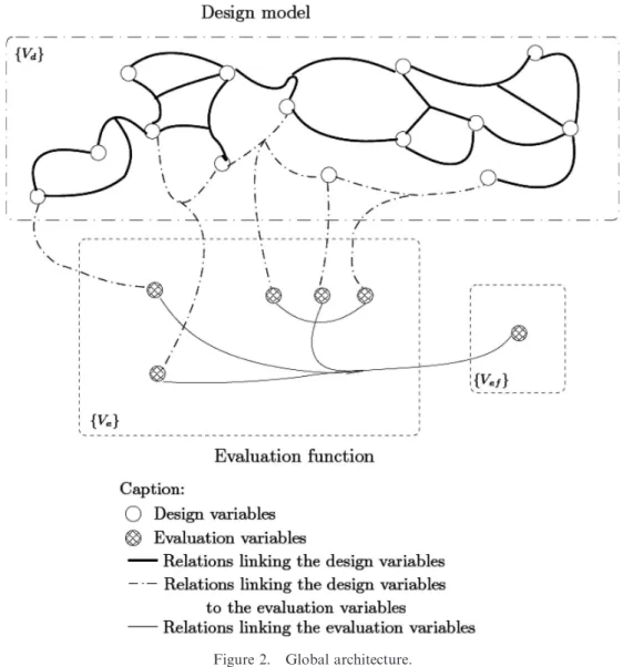
An aiding-design tool based on constraints corresponds to a design model and a model of the evaluation function,
as shown in figure 2. We assume that these two parts can be explicitly formulated from experts’ know-how. Therefore, two types of variables are considered (Vernat 2004): those belonging to the design model, denoted {Vd}, and those
belonging to the evaluation function, denoted {Ve}, as
shown in figure 2. The design variables {Vd} correspond to
the experts’ domain knowledge and also to technical feasibility, whereas the evaluation variables {Ve} are used
to compute the evaluation mark vefof the solutions.
3.1. Architecture of a constraints-based model
The design variables {Vd} can be either discrete or
continuous depending on the cardinal attribute of their domains. The domains of discrete variables are countable and defined as lists of symbols, integers or floats or as intervals of integers, whereas the domains of continuous variables are uncountable and defined as intervals of floats (Vareilles 2005). For instance, let v1be a numerical discrete
variable with domain {1, 2, [5, 45], 70}.
The design variables are linked with constraints such as mathematical formulae or compatibility tables which list all the permissible combinations of values for a set of variables. Let us look at the first compatibility table, c1,
of table 1. This compatibility table involves a pair of
variables vd2 and vd3 and tells us that the only two
permissible combinations of values for this pair are (?, 520) and (k, #20). These compatibility tables can be either discrete if they link only discrete variables, contin-uous if they link only contincontin-uous variables or mixed if they link discrete and continuous variables, as in our previous example (Gelle 1998).
The evaluation variables {Ve} are continuous and
defined within intervals of floats. The evaluation variables {Ve} are linked by the evaluation function that computes
the evaluation mark of a solution, the continuous vari-able vef.
The design {Vd} and the evaluation {Ve} variables are
most often linked together with mixed compatibility tables. Indeed, the combinations of values of the design variables has an impact on the evaluation mark of a solution.
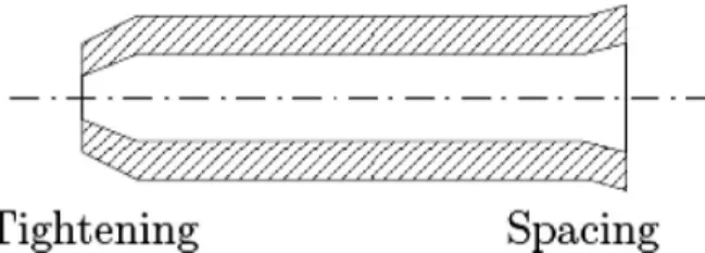
Let us consider an example from the industrial problem that is at the heart of our work: an axis with an inner hole, as shown in figure 3, the skin hardness of which must be improved by quenching in a particular medium. Unfortu-nately, during quenching, a negative effect corresponding to part distortion generally occurs. This occurrence depends on the design of the quenching operation. In this example we focus on the effect (1) of gravity, (2) of the quenching fluid direction—it can be either parallel or perpendicular to the part axis—and (3) of the position of the inner hole on the distortion intensity, which, in this particular problem, is the relevant data chosen to evaluate the quenching operation.
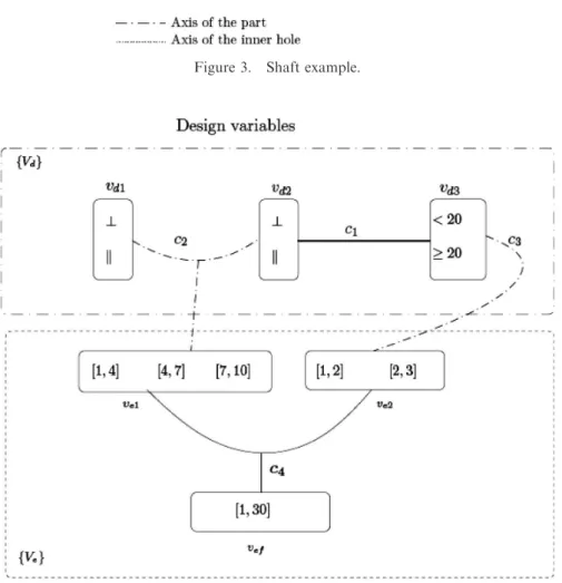
The associated network, presented in figure 4, is com-posed of:
. three design variables belonging to {Vd}: two
symbolic variables, vd1corresponding to the direction
of gravity versus the part axis, with domain Dvd1¼
{?, k}, and vd2, corresponding to the direction of the
quenching fluid versus the axis, with domain Dvd2 ¼ f?; kg, and one numerical discrete variable
vd3 corresponding to the axis gap, with domain
Dvd3 ¼ 0; þ1f½ g;
. three evaluation variables ve1, ve2 and vef with
domains Dve1¼ ½1; 10%f g; Dve2 ¼ ½1; 3%f g and Dvef¼
{[1, 30]}, respectively, which allow computation of the intensity of distortion;
. three compatibility tables, presented in table 1:
– one, c1, which is a mixed constraint between
two design variables vd2 and vd3
correspond-ing to the fact that the axis gap should be less than 20 if the quenching direction is perpen-dicular to the part axis, and greater than 20 otherwise,
Table 1. Compatibility constraint of the real example.
c1 c2 c3 vd2 vd3 vd1 vd2 ve1 vd3 ve2 ? 520 ? ? [7, 10] 520 [1, 2] k #20 ? k [4, 7] #20 [2, 3] k ? [4, 7] k k [1, 4]
– one, c2, which is a mixed constraint between two
design variables vd1 and vd2 and an evaluation
variable ve1 stating that the worst case
corre-sponds to the gravity and quenching fluid directions being perpendicular to the part axis,
whereas the best case is where both are parallel to it,
– one, c3, which is a mixed constraint between the
design variable vd3and an evaluation variable ve2,
stating that the worst case corresponds to an axis
Figure 3. Shaft example.
gap greater than 20, whereas the best case is where it is less than 20;
. one mathematical constraint, c4, computing the
evaluation mark:
vef¼ ve1& ve2:
3.2. Operating modes
Interactive aiding design consists of giving a value to or limiting the domain of a design variable vd. Modification of
the domain of vdis reflected through the constraints network
to the other design variables by retrieving all the values from their domain that are now inconsistent with the reduced domain of vd. This mechanism, repeated several times,
progressively restricts the solution space in order to reach a solution. In parallel, the evaluation mark is computed after each user’s input. With aiding design being interactive, we use the filtering techniques of constraints programming:
. discrete, mixed and continuous compatibility tables are filtered using arc-consistency (Mackworth 1977, Faltings 1994);
. mathematical formulae are filtered using 2B-consis-tency (Lhomme 1993), based on interval arithmetic (Moore 1966). Interval arithmetic extends real arithmetic to intervals by applying the operators of a formula to the endpoints of the intervals of its arguments. For example, if we consider the con-straint f : (x, y)7! x 6 y that adds the variables x to Dx¼ x; x½ % and y to Dy¼ y; y
h i
, the result of f yields Dx' Dy¼
½min fðx & yÞ; ðx & yÞ; ðx & yÞ; ðx & yÞg; maxfðx & yÞ; ðx & yÞ; ðx & yÞ; ðx & yÞg%:
Being based on constraints, which do not have propagat-ing directions, the knowledge model can be used in two operating modes. The first, called evaluation of a solution, consists of interactively inputting some restrictions on the design variables {Vd} in order to find a consistent solution,
simultaneously computing the evaluation mark vefof this
solution and comparing it with another one. The second mode, called choices deduced from an evaluation, consists of inputting restrictions on non-negotiable design variables belonging to {Vd} and a threshold on the evaluation mark vef
in order to deduce the value of the negotiable design variables of {Vd}. These two operating modes are illustrated by the
example presented in section 3.1 and by figure 3.
3.2.1. Evaluation of a solution. In the first operating mode, the user restricts the domain of the design variables {Vd} step by step to find a solution, the evaluation mark vef
of which is computed simultaneously.
Let us consider the example presented in subsection 3.1. At the start, as no choice has been made, the evaluation mark vefequals vef¼ ve16 ve2¼ [1, 10] 6 [1, 3] ¼ [1, 30].
If the user reduces the design variable vd1 to ?, this
reduction has a direct impact through the mixed constraint c2on the evaluation variable ve1, which is reduced to [4, 10].
The reduction of the evaluation variable ve1to [4, 10] has
an impact through the numerical constraint c4 on the
evaluation mark vef: vef is reduced to ðve1& ve2Þ \ Dvef¼
½4; 10% ' ½1; 3%
ð Þ \ ½1; 30% ¼ ½4; 30%.
If the user reduces the design variable vd2 to ?, this
reduction has a direct impact through the mixed constraint c2on the evaluation variable ve1, which is reduced to [7, 10].
The reduction of the design variable vd2 to ? has an
impact through the constraint c1on the design variable vd3,
which is reduced to520.
The reduction of the design variable vd3to520 has an
impact through the mixed constraint c3on the evaluation
variable ve2, which is reduced to [1, 2].
This reduction is reflected in the evaluation mark vef
through the numerical constraint c4 and reduces it to
ðve1& ve2Þ \ Dvef¼ ½7; 10% ' ½1; 2%ð Þ \ ½4; 30% ¼ ½7; 20%.
As the model is very simple, with only two user inputs, the problem is solved, vd1¼ ?, vd2¼ ?, vd35 20, and its
relevance is evaluated to [7, 20]. This solution is rather bad because we want to minimize the intensity of distortion and, in the worst case (vd1¼ ?, vd2¼ k, vd3# 20) the
relevance is evaluated to [8, 21] and in the best case (vd1¼ k,
vd2¼ k, vd3# 20) the relevance is evaluated to [2, 12].
3.2.2. Choices deduced from an evaluation. In the second operating mode, the user first gives a value to the non-negotiable design variables of Vdand then a threshold on
the evaluation mark vefin order to deduce the value of the
negotiable design variables belonging to Vd.
For instance, let us assume that the part geometry cannot be changed, therefore the axis gap is a non-negotiable variable. If the user reduces vd3 to 520, this
reduction has an impact through the constraint c1 on the
design variable vd2, which is reduced to?, and through the
constraint c3 on the evaluation variable ve2, which is
reduced to [1, 2].
The reduction of vd2 to ? is reflected through the
constraint c2 on the evaluation variable ve1, which is
reduced to [4, 10].
The reduction of ve2 and ve1 has an impact on the
evaluation mark vef through the numerical constraint
c4 and reduces it to ðve1&ve2Þ \ Dvef¼ ½4; 10% ' ½1; 2%ð Þ \
½1; 30% ¼ ½4; 20%.
As an example, let us now consider the case where the user reduces the evaluation mark vefto*6. This reduction
has a direct impact through the numerical constraint c4
on the evaluation variable ve1, which is reduced to
the evaluation variable ve2, which is reduced to ðvef=ve1Þ \ Dve2¼ ½4; 6% + ½2; 6%ð Þ \ ½1; 2% ¼ 2 3; 3 ! " .
The reduction of the evaluation variable ve1 to [2, 6] is
reflected through the mixed constraint c2 on the design
variable vd1, which is reduced tok. This reduction has no
impact.
The solution corresponding to vd35 20 with an
evalua-tion mark vef* 6 is vd1¼ k, vd2¼ ?.
3.3. Interests and limits
The first operating mode matches the expectations of the users: the design of the solution works well and the evaluation mark is computed after each user input in order to reach a final value. This operating mode allows a ‘what-if’ process in order to observe the impact of different choices on the relevance of the solutions and, therefore, it is very good for comparing different solutions.
The second operating mode can help the user solve her/ his problem by choosing ‘by her/himself’ coherent values for the negotiable design variables {Vd}. However, it can
lead to inconsistencies, which derive from 2B-consistency propagation. Like arc-consistency, 2B-consistency takes the numerical constraints into account sequentially.
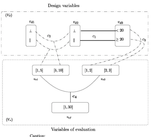
Let us consider the previous example, the constraint c2
of which is now simplified, as presented in table 2 and illustrated in figure 5, in order to illustrate this particular
Figure 5. Example of the limit of the second operating mode.
Table 2. Simplified c2constraint.
c2
vd1 vd2 ve1
? ? [5, 10]
limit. Now, at the start, as no choice has been made, the evaluation mark vef equals vef¼ ve16 ve2¼ [1, 10] 6
[1, 3]¼ [1, 30].
For instance, if the user reduces the evaluation mark vefto
52, this reduction has a direct impact through the num-erical constraint c4 on the evaluation variable ve1, which
is reduced to ðvef=ve2Þ \ Dve1¼ ½1; 2% + ½1; 3%ð Þ \ ½1; 10% ¼
1 3; 2
! ", and on the evaluation variable v
e2, which is reduced toðvef=ve1Þ \ Dve2 ¼ ½1; 2% + ½1; 10%ð Þ \ ½1; 3% ¼ 1 3; 2 3 ! " . The reduction of ve1to 13; 2 ! "
has an impact on the design variables vd1and vd2through the mixed constraint c2. These
two design variables are respectively reduced to k for ve1
andk for vd2. The reduction of vd2to 13;23
! "has an impact on the design variable vd3through the mixed constraint c3and
reduces it to520. The reduction of vd2tok has an impact
on the design variable vd3through the mixed constraint c1
and reduces it to ;. Indeed, the pair of values (vd2¼ k,
vd35 20) is not a permissible combination. The problem
does not have a solution.
Filtering with stronger consistency, such as 3B-consis-tency (Lhomme 1993), could avoid this problem, but it would be more time consuming and this is incompatible with an interactive aiding-design tool. This drawback can be avoided, however, by adopting a trial and error design.
4. Real example
We have developed such an aiding-design tool as part of a European project (project No. G1RD-CT-2002-00835) called VHT (Virtual Heat Treatment). This tool can, on the one hand, help users design heat treatment operations for steel parts and, on the other, evaluate the designed operations. A software mockup can be found on the Web at http://iena.enstimac.fr:20000/cgi-bin/vht.pl.
In this section we first present the industrial problem that is at the heart of our study, then one of the design models constructed with the experts involved in the project and, more specifically, the evaluation function they defined, and we end with an illustration of the two operating modes. The previous example presented in subsection 3.1 can be seen on the Web under the name IJCIM07.
4.1. Industrial problem
In order to improve the mechanical properties of steel, in particular the hardness of the surface, metallurgists treat it with a specific heat treatment operation called quenching. This heat treatment operation consists of three steps. The first step consists of heating a part up slowly in a furnace to a specific temperature called the austenite temperature. The second step consists of maintaining the part at this specific temperature to homogenize the steel micro-structure. The last step consists of the rapid cooling of the part by plunging it into a specific medium such as air, water or oil.
The expected effect of this heat treatment is an improve-ment in the hardness of the surface of the part but, unfortunately, a negative effect, distortion of the part, usually occurs at the same time.
A means of evaluating distortion is behaviour simulation using Finite Element Method Codes (FEM). They make it possible to obtain a quantitative prediction of the distor-tion at the design stage. However, the tools are costly, time consuming and very complicated to use, due to the mechanical/structural/thermal behaviour and data require-ments. The situation is becoming even more difficult in the current context of smaller production series and the high reactivity of the market. Furthermore, the relevance of the solutions can be the result of some expert’s interpretation of many (up to 20) modifications of the dimensions, therefore it is very difficult for a non-expert user to compare different solutions. That is why, more often than not, the design of a quenching heat treatment that minimizes distortion relies on the know-how of experts.
There is a real need for metallurgists to make good decisions without the use of behaviour simulations. Only a few recent studies have used experts’ know-how to help them to make better decisions: Varde et al. (2003) used an Expert System to model knowledge and design heat treatment operations with a trial and error procedure, whereas Klein et al. (2005) studied different techniques, such as artificial neural networks or fuzzy logic, to develop a prognosis tool. In this European project, two domain knowledge simulation tools have been developed:
. a CBR tool exploiting implicit domain knowledge, which will not be detailed in this paper. With this tool, each past case is described by 250 relevant parameters. A software mockup can be seen on the Web at http://hefaistos.ivf.se/IMS-VHT/GUI/Gen-eral.html. This kind of tool is very useful for large companies that always have the same kind of parts to treat, such as the automobile industry. For example, the partner Scania is a good representative of this kind of user. Indeed, a CBR needs many, similar past cases to retrieve those that are nearest to that being considered;
. a tool based on constraints exploiting explicit domain knowledge. A software mockup can be seen on the Web at http://iena.enstimac.fr:20000/cgi-bin/vht.pl. This kind of tool is more useful for heat and surface treatment providers that treat a large variety of parts and need experts’ advice for all the different kinds of shapes. For example, the partner Metallographica is a good representative of this kind of user.
In order to develop a tool based on constraints, we have extracted and collected experts’ knowledge over the last three years. Inspired by certain design literature models,
such as that of Oliveria et al. (1986), two intermediate reasoning models based on constraints have been con-structed (David et al. 2003) and have led to an advanced model (Aldanondo et al. 2005). In this latter model, many of the constraints resulting from experts’ know-how have been validated by other academic partners of the project. These validations have been done either by simulations with FEM codes or by real experiments.
In our application, the experts defined the relevance of the solutions as an evaluation mark Vefcorresponding to a
qualitative intensity of distortion If. As the characterization
of a unique intensity of distortion Ifis very complicated to
identify for any kind of part, the experts shared out the different shapes to several families of parts, such as axes, disc or gears. First, they focused on the family of axes, which is most often treated by the metallurgists involved in the project.
The definition of a unique intensity of distortion Ifis also
very difficult to estimate for a particular part family because the geometry of the part can consist of several features. For instance, an axis can have holes, shoulders and/or variations of thickness, which all have a different impact on the intensity of the distortion If. Experts have
established that the unique intensity of distortion Iffor axes
must be decomposed into five distortion intensities, denoted Ii
f, corresponding to five distortion components
gathered in a distortion vector, denoted Di(Lamesle et al.
2005). These five distortion intensities are
. I1
f, corresponding to the intensity of distortion
following a ‘banana’ shape. For some reason, due essentially to the direction of the quenching medium and the existence of dissymmetry, an axis can be deformed as a banana, as shown in figure 6;
. I2
f, corresponding to the intensity of distortion
following a ‘spool-barrel’ shape. For metallurgical reasons, an axis can be deformed as a spool or a barrel, as shown in figure 7;
. I3
f, corresponding to the intensity of distortion
following a ‘spacing-tightening’ shape. If there is at least one hole at one of the extremities of the axis, a spacing or a tightening can be observed, as shown in figure 8;
. I4
f, corresponding to the intensity of distortion
following an ‘ovalization’ shape. If there is a circular hole along the axis and if the axis is not supported, this circular hole can become oval, as shown in figure 9;
. I5
f, corresponding to the intensity of distortion
following an ‘umbrella’ shape. If there is a shoulder on the axis, this shoulder can be deformed as an ‘umbrella’, as shown in figure 10.
Experts have decided to give a range of [1,1000] to each intensity of distortion Ii
f: a value of 1 corresponds to the
lowest intensity of distortion, whereas a value of 1000 is the highest intensity.
4.2. Knowledge model
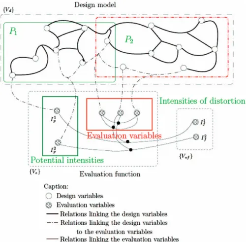
The knowledge model is composed of two parts: the first is used to design the heat treatment operation and the second to compute the evaluation function, as shown in figure 11.
Experts have defined the evaluation function for each intensity of distortion Ii
f as the product of the potential
intensity of distortion Ii
p using a set of evaluation
variables vej:
Ii
f¼ Ipi& ve1& , , , & vej:
A potential distortion intensity Ii
p is associated with each
distortion intensity Ii
f and allows a first evaluation of the
corresponding distortion intensity Ii
f. A set of 30 design
variables vd, denoted P1, are used to compute the value of
Figure 6. ‘Banana’ distortion component.
the five potential intensities of distortion Ii
p. These design
variables mainly characterize:
. the axis geometry: thickness, diameter, existence of shoulders and holes, etc.;
. the resources used for the operation:
– the position and the wedging of the axis:
suspended, supported, etc.,
– the direction of the quenching medium, either
perpendicular or parallel to the axis,
– the direction of gravity, either perpendicular or parallel to the axis,
– the steel: 30CrNiMo8, 42CrMo4, 90MnV8, etc.
For instance, let us consider the compatibility table 3, which allows us to compute the potential intensity of distortion following a ‘banana’ shape I1
p. This intensity is
characterized by the direction of the quenching medium Dqm, by the direction of gravity Dgand by the position and
wedging of the axis Pa. Each value of this potential
intensity corresponds to a combination of values of the subset of the designed variables belonging to P1.
It can be seen from figure 11 that each potential distortion intensity Ii
p results from a different part of the
design model.
Around 30 evaluation variables vejincrease or decrease
the value of the potential distortion intensity Ii
pin order to
compute the evaluation mark Ii
f. A set of 70 design
variables vd, denoted P2, are used to compute the value
of these evaluation variables vej. Experts have apportioned
these variables into six groups, characterizing:
. the quenching medium: gas, water, air, oil, drasticity, temperature, etc.;
. load preparation: basket permeability, symmetry around the part, etc.;
. the general geometry of the axis: thickness variation, degree of dissymmetry, etc.;
. the metallurgical characteristics: material trempabil-ity, carburizing, etc.;
. the material history: forming process, relaxation, etc.; . the heating cycle: furnace class, heating speed, etc. For instance, let us consider the compatibility table 4, which allows us to compute the evaluation variable ve12.
This evaluation variable is characterized by the quench-ing medium Qm and by the thickness variation Tv of the part. Each value of the evaluation variable corre-sponds to a combination of values of the subset of de-signed variables belonging to P2, showing that a liquid
quenching fluid is better than a gas fluid and that a small thickness variation has a small impact on the intensity of distortion.
It is worth stressing that a very small subset of design variables belongs simultaneously to subsets P1and P2and
that the constraints between the variables of P1 and P2
correspond to technical feasibilities. P1 and P2 are not
differentiated for users: they reduce indifferently the domains of the design variables belonging to P1 and P2
indifferently.
As each distortion intensity Ii
fmust belong to the interval
[1, 1000] and is computed from the product of its potential distortion attribute Ii
p by a specific set of evaluation
variables vej, the influence of the two subsets of design
Figure 8. ‘Spacing-tightening’ distortion component.
Figure 9. ‘Ovalization’ distortion component.
variables P1and P2have been analysed by experts. Their
influences result from experts’ know-how:
. the influence of P1on the final intensity of distortion
has been fixed at 30%: each potential distortion attribute Ii
pbelongs to the interval [1, 20];
. the influence of P2has been fixed at 70%: the product
of all the evaluation variables vejbelongs to the interval
[1, 50]. As subset P2is composed of six groups, the
influence of each was also determined by the experts:
– 35% for the group characterizing the quenching
medium,
– 20% for the group characterizing the load
preparation,
– 15% for the group characterizing the general
geometry, Figure 11. Architecture of the knowledge model.
Table 3. Characterization of the potential intensity of the ‘banana’-shape distortion.
Dqm Dg Pa I1p
Parallel Parallel Suspended 1 Parallel Parallel Supported [1, 2.3] Parallel Perpendicular Good chock [2.3, 4.3] Parallel Perpendicular Bad chock [4.3, 6.2] Perpendicular Parallel Suspended [7.9, 8.9] Perpendicular Parallel Supported [8.9, 10.2] Perpendicular Perpendicular Good chock [10.2, 11.5] Perpendicular Perpendicular Bad chock [12.8, 14.1]
Table 4. Characterization of the evaluation variable ve12.
Tv Qm ve12 41.5 Water [10, 12] [1,1.5] Water [8, 10] 51 Water [7, 8] 41.5 Oil [5, 7] [1,1.5] Oil [3, 5] 51 Oil [2.5, 3] 41.5 Air [1.8, 2.5] [1,1.5] Air [1.2, 1.8] 51 Air 1.2
– 15% for the group characterizing the metallurgi-cal characteristics,
– 10% for the group characterizing the material
history,
– and 5% for the group characterizing the heating cycle.
To synthesize, the final reasoning model is composed of . five distortion components Di;
. five potential distortion intensities Ii
pbelonging to the
interval [1, 20];
. five distortion intensities Ii
fequal to the product of Ipi
and vejand belonging to the interval [1, 1000];
. around 90 design variables with 30 belonging to
P1, which allow us to compute the potential
distortion intensity Ii
p, and 70 belonging to P2,
which are linked to a set of 30 evaluation variables vejto compute the evaluation mark of the designed
solution;
. around 10 discrete, 30 mixed and 10 continuous compatibility tables;
. around 60 mathematical constraints to compute the final evaluation marks and to allow the use of the model with the two operating modes.
4.3. Operating modes
The first operating mode lives up to the metallurgists’ expectations: the design choices are well reflected in the variable domains, laid to a consistent heat treatment operation, and the intensities of distortion Ii
f of each
distortion component are in agreement with the prediction of the metallurgists.
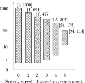
After each user’s input, the distortion intensities Ii f are
progressively reduced. We can see from figure 12 that the evolution of the distortion intensity follows one of the distortion components: the ‘spool-barrel’. Before any choice is made, this intensity belongs to [1, 1000] (time (0)) and decreases after each user input:
(i) description of the part geometry (time (1)); (ii) description of the load preparation (time (2)); (iii) description of the material history (time (3)); (iv) description of the metallurgical characteristics
(time (4));
(v) and description of the quenching fluid (time (5)). Therefore, the simultaneous design/evaluation permits a ‘what-if’ decision aid.
If, in the previous example, a threshold is given to the intensity of distortion of the ‘spool-barrel’ component after a complete description of the material history (time 3), e.g. distortion 550 as shown in figure 13, the selection of a
quenching fluid is done automatically by the system: oil. As pointed out in section 3.3, the second operating mode can lead to inconsistent solutions if the thresholds on the distortion intensities Ii
f are too strong.
A drawback of the model has also been identified by the experts: in all the models developed using experts, only the minimization of the distortion is actually taken into account. Then, when a user designs a heat treatment operation in order to minimize the intensity of distortion, the solution reached effectively minimizes the distortion, but sometimes does not improve the mechanical properties of the part. We have to improve our models by adding another relevant component representing the improvement of the mechanical properties. The user will then have to come to an agreement concerning the improvement of the mechanical properties and the minimization of the resulting distortion.
4.4. Synthesis
In order to develop the reasoning models presented in the previous section, we have extracted and collected experts’ knowledge over three years. During this time, an advanced model has been constructed for a specific family of parts, axes, and it still needs some improvements before being completed.
The extraction and validation of the knowledge are always lengthy and difficult and even more so when the knowledge is not always available, accessible, easy to validate and to formalize. Furthermore, the problem of maintenance of the models is crucial: some knowledge is stable and some is not. In order to maintain the models we have to identify both the stability of the knowledge and the necessary frequency of maintenance.
This kind of tool is easier to develop if the object of study is fairly routine because the knowledge is more stable and therefore easier to identify, to extract and also to maintain. This was the case in our application.
5. Conclusion
The aim of this paper has been to show how the relevance of solutions can be estimated or evaluated in an interactive aiding-design process in order to help users to make better decisions.
First we compared how the solutions can be evaluated by two means: behaviour simulations and domain knowl-edge simulations. Behaviour simulations retrieve the ‘best’ solution following several criteria. It is the user who has to determine the relevance of the solution. For domain knowledge simulations, CBR, ES and CSP, there is usually no method for evaluating the solutions for a non-expert user. We have therefore concentrated our study on domain knowledge simulations in order to fill this gap.
We identified three different methods of evaluating solutions in domain knowledge simulations:
. identification of a small set of relevant and indepen-dent data. In this case, the evaluation is embodied in the system;
. definition of an explicit evaluation function defined by experts which must be added to the system; . learning from past experiments using an ANN which
is added to the system; . or regression analysis.
We have focused on constraints-based systems because of their consistent properties, their ability to model experts’
knowledge and for their ability to be easily understood. As this kind of model is based on the extraction of experts’ know-how, for its translation into constraints and its validation, we have assumed that experts are able to determine the set of data to be taken into account and how to combine them in order to define an explicit evaluation function. The constraints-based system is then composed of two different parts: one which helps the user to design her/ his solution, and the other which evaluates the solution.
Being based on constraints, which do not have propagat-ing directions, the knowledge model can be used in two operating modes. The first, evaluation of a solution, consists of interactively inputting restrictions on the design vari-ables in order to find a coherent solution and of simultaneously evaluating the solution. The second mode, choices deduced from an evaluation, consists of inputting restrictions on non-negotiable design variables and a threshold on the evaluation in order to achieve values for the negotiable design variables.
This kind of approach has been used in a real problem to help users design and evaluate heat treatment operations. This tool is appreciated by the users because:
. it is very useful for comparing solutions, although it is somewhat weak for comparing different solutions in an absolute way;
. it is very useful for observing the consequences of a decision in a ‘what-if’ process;
. although the second operating mode is somewhat tricky to use, it is much appreciated by users in helping them complete a heat treatment operation design.
We are currently working on improvements to our design models in order to take into account the mechanical Figure 13. Selection of a negotiable variable.
properties of steel and on improvements of the ergonomics of the Web mockup in order to make it more user-friendly. Acknowledgements
This work was partly funded by the European Commission through the IMS project. The authors wish to acknowledge the Commission for their support. We also wish to acknowledge our gratitude and appreciation to all the VHT project partners (especially EMTT (France), SCC (France), Metallographica (Spain), Scania (Sweden) and IWT (Germany)) for their contribution during the devel-opment of the various ideas and concepts presented in this paper. This paper is an extended version of that in the proceedings volume from the 12th IFAC International Symposium on Information Control Problems in Manu-facturing (INCOM’06) (ISBN: 978-0-08-044654-7, Elsevier Science, Saint Etienne, France, December 2006).
References
Aldanondo, M., Vareilles, E., Lamesle, P., Hadj-Hamou, K. and Gaborit, P., Interactive configuration and evaluation of a heat treatment operation, in Workshop on Configuration, International Joint Conference on Artificial Intelligence, 2005.
Banks, J., Carson, J. and Nelson, B., Discrete-event System Simulation (International Series in Industrial and Systems Engineering), 1984 (Prentice-Hall: Englewood Cliffs, NJ).
Bouzeghoub, M., Gardarin, G. and Metais, E., Database design tools: an expert system approach, in 11th International Conference on Very Large Data Bases, 1985, pp. 82–95.
Buchanan, B-G. and Shortliffe, E-H., Rule-based Expert Systems, the Mycin Experiments of a Stanford Heuristic Programming Project, 1984 (Addison-Wesley: Reading, MA).
David, P., Veaux, M., Vareilles, E. and Maury, J., Virtual heat treatment tool for monitoring and optimising heat treatment, in 2nd International Conference on Thermal Process Modelling and Computer Simulation, 2003.
Dechter, R., From local to global consistence. Artif. Intell., 1992, 87–107. Faltings, B., Arc consistency for continuous variables. Artif. Intell., 1994,
363–376.
Fu, M., Optimization for simulation: theory vs. practice. INFORMS J. Comput., 2002, 14, 192–215.
Gelle, E., On the generation of locally consistent solution spaces in mixed dynamic constraint problems. PhD thesis, E´cole Polytechnique Fe´de´rale de Lausanne, Suisse, 1998.
Huang, G.Q., Design for X-Concurrent Engineering Imperatives, 1996 (Springer: Berlin).
Klein, D., Thoben, K-D. and Nowag, L., Using indicators to describe distortion along a process chain, in International Conference on Distortion Engineering, 2005.
Kolodner, J., Case-based Reasoning, 1993 (Morgan Kaufmann). Lamesle, P., Vareilles, E. and Aldanondo, P., Towards a KBS for a
qualitative distortion’s prediction for heat treatments, in International Conference on Distortion Engineering, 2005.
Lhomme, O., Consistency techniques for numeric CSP, in International Joint Conference on Artificial Intelligence, 1993, pp. 232–238. Mackworth, A.K., Consistency in networks of relations. Artif. Intell., 1977,
99–118.
Magrab, E-B., Integrated Product and Process Design and Development, 1997 (CRC Press: New York).
Maher, M., Zhang, D. and Balachandran, M., Case-based Reasoning in Design, 1995 (Lawrence Erlbaum Associates).
Minsky, M. and Papert, S., Perceptrons, 1969 (MIT Press: Cambridge). Montanari, U., Networks of constraints: fundamental properties and
application to picture processing. Inf. Sci., 1974, 7, 95–132.
Moore, R.E., Interval Analysis, 1966 (Prentice-Hall: Englewood Cliffs, NJ). Oliveira, M., Moreira, A., Loureiro, A.P., Denis, S. and Simon, A., Effet du mode de refroidissement sur les de´formations produites par la trempe martensitique, in 5th Congre`s International sur les Traitements Thermi-ques des Mate´riaux, 1986.
Riesbeck, E-l. and Shank, R., Inside Case-based Reasoning, 1989 (Lawrence Erlbaum Associates: NJ).
Szabo, B. and Babuska, I., Finite Element Analysis, 1991 (Wiley: New York).
Tsang, E., Foundations of Constraints Satisfaction, 1993 (Academic Press: London).
Tsatsoulis, C., A review of artificial intelligence in simulation. ACM SIGART Bull., 1990, 2, 115–121.
Varde, A., Maniruzzaman, M., Rundensteiner, E. and Richard, D., The QuenchMiner expert system for quenching and distortion control, in ASM’s HTS-03, 2003, pp. 174–183.
Vareilles, E´., Conception et approches par propagation de contraintes: contribution la mise en oeuvre d’un outil d’aide interactif. PhD thesis, E´cole des mines, Albi-Carmaux, France, 2005.
Vernat, Y., Formalisation et qualification de mode`les par contraintes en conception pre´liminaire. PhD thesis, E´cole Nationale des Arts et Me´tier, Bordeaux, France, 2004.