Hydraulic modelling for assessment of the performance of sedimentation basins downstream from extracted peatlands.

sedimentation basins downstream from extracted peatlands

S. Hafdhi, S. Duchesne, A. St-Hilaire

Research Centre on Water, Earth, and the Environment (INRS-ETE), Quebec City, Canada

_______________________________________________________________________________________

SUMMARY

Three sedimentation basins on two different extracted peatlands were studied to determine their Trapping Efficiency (TE) using two different methods. First, TE was calculated using sediment loads estimated from turbidity measurements upstream and downstream of the basins. The second method was based on hydraulic modelling and a simplified sediment deposition model. For the first studied basin (controlled by a weir at its downstream end) TE was estimated with the second method at 85.9 % and 55.6 % for lower and higher flows, respectively. In the second peatland the studied basins were in series, there was a geotextile curtain in the middle of each basin and a weir or a double pipe culvert at the outlet. For these two basins in series, TE was estimated at 80 % for lower flows and at 34.3 % for higher flows. A hydraulic model was calibrated for the studied basins and applied to estimate the TE of different basin configurations. The results show that the role of the geotextile curtain is important in the case of short basins and for intense rainfall events. The double pipe culvert did not have a significant effect on TE, unlike the presence of a weir at the outlet, which is required to maintain high TE.

KEY WORDS: deposition model, field data, HEC-RAS, suspended solids, trapping efficiency

_______________________________________________________________________________________

INTRODUCTION

Canada is one of the largest producers of horticultural peat in the world. Peatlands cover 11.4 % of the country’s total area, or about 113.4 million hectares, with 11.2 million ha located in the province of Quebec (about 7.2 % of the province’s territory) (Daigle & Gautreau-Daigle 2001). These peatlands are poorly drained ecosystems where significant amounts of vegetation accumulate and decompose very slowly under anaerobic conditions to form peat. There are different types of peatlands, including ombrotrophic peatlands which are also called bogs. These bogs constitute an acidic environment where vegetation is dominated by Sphagnum mosses. Solutes (plant nutrients) and water supply come essentially from precipitation and atmospheric deposition (Landry & Rochefort 2011). The peat extracted from these peatlands is a sought-after product, mainly for use in growing media for horticulture, thanks to its water and mineral retention qualities. For the Canadian industry, only bogs larger than 50 ha with a peat thickness greater than 2 m are considered profitable (Cris et al. 2014).

To extract peat from peatlands, the first step is to remove vegetation from the operating area to expose the underlying peat. Then, aiming to lower the water table, parallel drainage ditches are dug (Clément et al. 2009). Drained water, sometimes loaded with

suspended matter, is subsequently collected in a deeper main channel and conveyed to a sedimentation basin before being discharged into a nearby watercourse. The main goal of sedimentation basins is the retention of suspended sediments and, thus, the reduction of sediment loads conveyed to the receiving watercourse (Pavey et al. 2007). The main problem relating to peat drainage is the possibility of negative environmental effects on natural streams receiving drainage waters that are rich in suspended matter. The continuous release of suspended solids from peatlands where peat extraction is ongoing can lead to eutrophication and siltation downstream (Marttila & Kløve 2008). The effect of suspended sediments depends on the characteristics of the receiving environment as well as on the volume, concentration and composition of the discharged water (Benyahya et al. 2003). Suspended sediments can affect the flora and fauna of the receiving environments by influencing the dynamics of the benthic community (Vuori & Joensuu 1996, Schofield et al. 2004) and the species composition of algae, and thus affecting the organisms that feed on them (Schofield et al. 2004) as well as the fish population (Laine 2001). Suspended sediments can carry contaminants and phosphorus (Paavilainen & Päivänen 1995), with the latter possibly contributing to eutrophication. Finally, decomposition of the organic fraction of suspended solids leads to oxygen

consumption in the watercourse (Landry & Rochefort 2011).

Trapping Efficiency (TE), reflecting the proportion of sediments trapped in the sedimentation basin, can be calculated in several ways (Verstraeten & Poesen 2000). These methods require suspended sediment measurements upstream and downstream of the studied basin (Verstraeten & Poesen 2000). Many predictive models of the efficiency of basins in retaining mineral sediments are available from the literature. Brown (1943) developed an empirical nonlinear model relating TE to the quotient of basin volume and drained area (C/W) using data from 15 reservoirs. However, Brown’s model does not provide a good fit to data from basins with low C/W (Brune 1953). To overcome this problem, Brune (1953) developed a model based on the relationship between TE and the quotient of basin volume and inflow (C/I) using data from 44 reservoirs (Verstraeten & Poesen 2000). Brune’s model does not take into consideration the reservoir dynamics, leading to over-estimation of TE in some cases (Trimble & Bube 1990). Heinemarm (1981) modified Brune’s model and used it for 20 small ponds (with catchment areas smaller than 36.3 km²) (Verstraeten & Poesen 2000). Samson-Dô & St-Hilaire (2018) adapted Brown’s model (tested on four basins) and Heinemarm’s model (tested on six basins) for sedimentation basins on harvested peatlands and concluded that the high TE for multiple basin configurations may not be attributable solely to their high C/W or C/I values. However, the methods mentioned above do not take into account flow dynamics, nor do they allow TE to be assessed after making changes to the basins.

The main objective of this article is to evaluate the suspended solids retention efficiency of various sedimentation basin configurations, and of related

sediments and flow control structures (geotextile curtain and double pipe culvert) in this context, using hydraulic modelling. The evaluation is performed using a hydraulic model (HEC-RAS) and data collected during four months on two different peatlands in the province of Quebec (Canada).

METHODS

Monitoring instruments were installed in two peatlands from May to October 2017 to collect rain, turbidity, water level and flow data upstream and downstream of three sedimentation basins. The sites were monitored from May to October because ditches and basins are frozen in winter and the study sites are not accessible during the snowmelt period (impassable access roads). Turbidity and flows were used to calculate TE, while water levels and flows were used to calibrate the HEC-RAS hydraulic model for each studied basin. Flow velocities in the basins, simulated by the model, were used to evaluate TE with a simplified deposition model. TE was also evaluated with this model for various basin configurations. More details are given below.

Description of the sites and stations

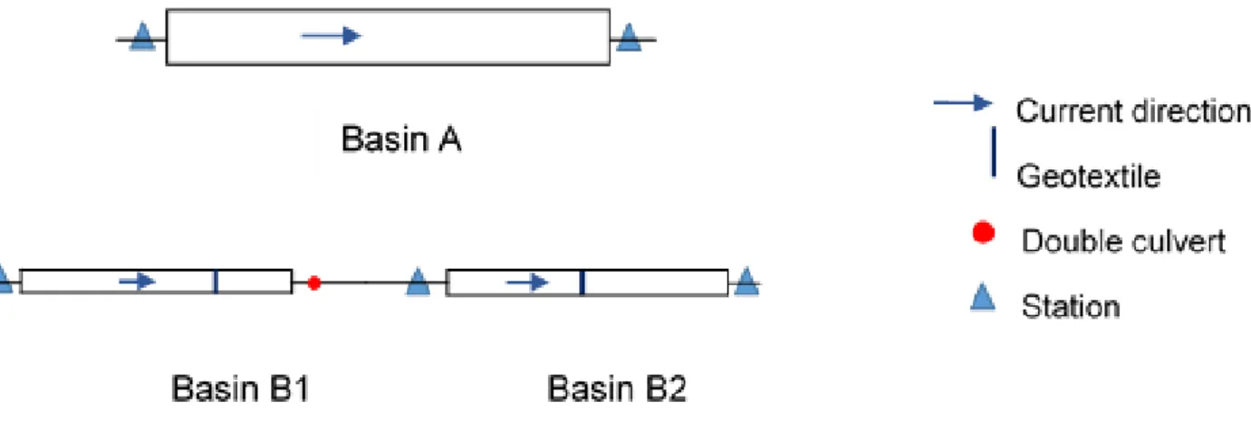
Two peatlands (ombrotrophic bogs) located in the Province of Quebec (Canada) were studied. In the first peatland (Peatland A), one simple rock-lined basin (Basin A; Figure 1 and Figure 2g) was studied. A weir controls the output of this basin (Table 1) and the total drained area is 66 ha (Samson-Dô & St-Hilaire 2018). Basin A was dug in a sandy soil and it was riprapped to ensure bank stability.

In the second peatland (Peatland B), two basins were studied (Figure 1 and Figure 2a–f). These basins were dug in peat underlain by clay soil. The upstream

Figure 1. Diagram of the three basins studied, with the positions of water and sediment retention structures and stations. For dimensions and other characteristics of the basins, see Table 1 and Table A1 (Appendix).

basin (B1) contains sediment and flow control structures of two types: a suspended geotextile curtain in the middle of the basin and a weir with a double pipe culvert at the outlet (Table 1). The lower part of the double pipe culvert controls the outflow of water during low flows, while the upper one controls higher flows (Figure 2b,c,d). The second basin, Basin B2, is located downstream of Basin B1. This basin contains a suspended geotextile curtain 30 m

from the inlet (Figure 2f). A ditch 34.3 m long connects the two basins (Figure 2e). The total area drained by Basin B1 and Basin B2 is 23 ha (Samson-Dô & St-Hilaire 2018).

The von Post scale was used to estimate the degree of decomposition of peat. This scale distinguishes ten categories from H1 (completely undecomposed peat) to H10 (completely decomposed peat) (Stanek & Silc 1977). The von

Figure 2. (a) Inflow channel and Basin B1; (b) geotextile in Basin B1; (c) (d) double pipe culvert; (e) channel connecting Basin B1 and Basin B2; (f) Basin B2 with the geotextile in the middle and the output canal; (g) Basin A.

Post values are H3 for Peatland A and H6 for Peatland B (source: managers of the peat extraction enterprises), which means that organic matter is more decomposed in Peatland B than in Peatland A and, therefore, the settling velocity of particles in Basins B1 and B2 should be lower than in Basin A.

In 2017, five monitoring stations were installed: two stations in Peatland A, upstream and downstream of Basin A; and three stations in Peatland B, one upstream of Basin B1, the second between Basin B1 and Basin B2 (in the connecting canal) and the third downstream of B2 (Figure 1).

At each station an Optical Back Scatterometer OBS -3+ turbidity sensor (manufacturer: Campbell Scientific, USA), attached to a metal rod, was installed in the water column. A mechanical wiper system (Hydro Wiper, Zebra-Tech Ltd., New Zealand) was attached to the turbidity probe to prevent obstruction of the optical window by mud and debris. The hydro brush was set to clean the sensor every 30 minutes. The turbidity sensor was linked to a Campbell Scientific Datalogger (CR1000) which recorded the signal from the probe every 30 s and calculated its average over 15 min time intervals. The signal from the OBS +3- submersible sensor (volts) was converted to suspended sediment (SS) concentration (SS; mg L-1_{) using a calibration curve}

specific to each station, following the protocol described by Pavey et al. (2007) (see Table A1 in Appendix).

A pressure transducer (HOBO U20 Series) was installed in a deeper part of the ditch at each station, in a perforated PVC tube covered with nylon stockings to prevent clogging by fine sediments. One additional pressure transducer was installed in each peatland to measure air pressure. The recording interval for all pressure transducers was 15 min. The data were used to derive a 15 min water level record for each station.

Liquid precipitation was recorded by a tipping bucket raingauge (TB3, HyQuest Solutions, Germany) installed in each peatland. The raingauge was linked to the Campbell Scientific Datalogger and total precipitation was recorded every 15 min.

Field measurements

Calibration

The Optical Back Scatterometer is a dual range sensor (low and high range output) that measures turbidity indirectly in the water column. A station-specific calibration curve was used to convert the voltage signal measurements to suspended solids concentrations (e.g. Figure A1). If the signal was below 2.5 V, the calibration curve for low range output was used; if not, SS was calculated using the calibration curve for high range output. The calibration was done in situ for each probe using water and sediments collected from the sites. The use of in situ water and sediments ensures that the water colour and the dissolved organic carbon content of grab samples represents those of drainage water on the study sites. A rectangular container was filled with water, then sediments with median diameter <500 microns were added and kept in suspension by manually stirring until the voltage was measured and a grab sample of water was taken. This allowed the calibration curve to cover the whole range of possible SS values, which would not be possible if only spot samples of drainage water were used, due to the difficulty of synchronising the field visits with important SS events. A water sample (at least 750 ml) was collected at each of at least ten turbidity levels for each station. Each water sample was filtered using a ProWeight TM 11 cm filter (1.2 µm pore size) and the residue retained by the filter was dried in an oven for one day. After determining the weight of sediment in each sample, and knowing the associated

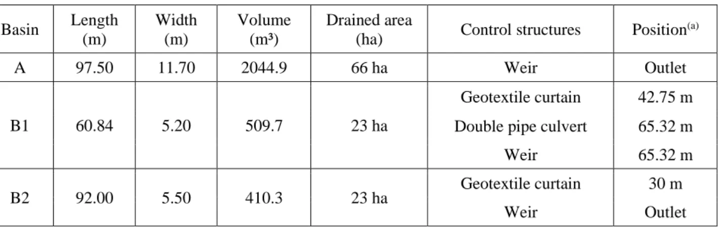
Table 1. Characteristics of the studied basins.

Basin Length (m) Width (m) Volume (m³) Drained area

(ha) Control structures Position

(a)

A 97.50 11.70 2044.9 66 ha Weir Outlet

B1 60.84 5.20 509.7 23 ha

Geotextile curtain 42.75 m Double pipe culvert 65.32 m

Weir 65.32 m

B2 92.00 5.50 410.3 23 ha Geotextile curtain 30 m

Weir Outlet

voltage outputs, the calibration curve was constructed and the equation was used to convert the series of turbidity measurements collected from May to October 2017 into SS concentrations (see Table A1 for equations).

Flow measurements and precipitation

During the monitoring period, all sites were visited regularly to check the equipment and download data. At each station and at different times during the field season, velocity measurements were performed across the inflow and outflow ditch sections using a Marsh McBirney Flo-Mate 2000 velocimeter and flow was estimated by the velocity-area method. At the end of the field season, a rating curve was established for each station (e.g. Figure A2). Using that curve, level measurements were converted into a flow time series (see Table A1 for equations).

Daily precipitation data were obtained at the end of the season for each studied peatland. The maximum daily precipitation recorded for Peatland A was 44.3 mm, corresponding to the rainfall event of 27 September 2017. At Peatland A, total precipitation for the season was 491.6 mm. Precipitation was lower at Peatland B than at Peatland A. Total precipitation for the season was underestimated on-site at Peatland B because the raingauge was blocked by peat at the end of the season. In this case, rainfall data from a measuring station located 8 km from Peatland B were used. At this station, the total rainfall during the same period was 449 mm.

Hydraulic modelling of studied basins

HEC-RAS 5.0 (Brunner 2016) was used to create one-dimensional simulations of water surface profiles and flow velocities in each studied basin, using the series of observed upstream flow as input data. Although two- or three-dimensional simulations would have provided a more detailed description of water velocities, the mean water velocity provided by the one-dimensional HEC-RAS model was considered sufficient to estimate the quantity of SS deposited in the basins during the simulation periods and, thus, to compute the seasonal TE. The steady flow simulation was chosen since flow usually varies smoothly in the studied basins. Further details for unidirectional modelling using HEC-RAS can be found in the HEC-RAS 5.0 Reference Manual (Brunner 2016).

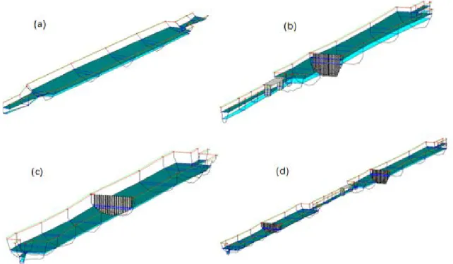
For Basin A, flow velocity was generally low with flow depths above the critical depth, so the subcritical regime (Froude number less than 1, impact on water levels from downstream to upstream) was chosen for the simulation. The hydraulic model of Basin A was formed by seven sections (the locations of the sections being determined mainly by their accessibility for measurement of bathymetry), with an average distance between sections of 13.9 m (Figure 3a). For Basins B1 and B2, the model was run in a mixed flow regime (either subcritical or super- critical depending on flow conditions, since both subcritical and super-critical flow regimes were encountered in the simulation series). The hydraulic

Figure 3. Hydraulic models for (a) Basin A; (b) Basin B1; (c) Basin B2; and (d) Basins B1–B2 (in series), showing the lowest (cyan) and highest (green) simulated water surface.

models for Basins B1 (Figure 3b) and B2 (Figure 3c) were composed of 13 and 9 sections, respectively, with an average distance between sections of about 7.5 m for Basin B1 and 6.15 m for Basin B2. When the hydraulic models of these basins had been validated individually, a hydraulic model of the two basins in series was developed (Figure 3d).

For both studied peatlands, the input data to start the simulation were: series of flow data upstream of the basins (termed “profiles” in HEC-RAS), geometry data (length, width, depth), and the basin altitude(s). Manning’s roughness coefficient (n) and the friction slope (Sf) were the calibration parameters. The output data needed to determine the efficiency of the basins were the water flow velocities at every section of each basin.

For steady flow, the input flow constitutes the boundary condition upstream of the studied basin. For Basin A, the boundary condition downstream of the basin (required because of the subcritical regime) was set to normal depth. For Basins B1 and B2, normal depth both upstream and downstream of the basins was needed.

Flow data and water levels for 2017 were used to calibrate and validate the models. The series of lowest and highest flow values were used to determine n and Sf. Then the rest of the 2017 series of flow data was used for validation of the hydraulic models.

For Basin A, the total series of flow (Q) data obtained from May to October 2017 contained 3508 hourly flow values. Of these, 168 were lower than 0.0187 m³ s-1 _{(Percentile 40, low Q) and 152 were}

greater than 0.0468 m³ s-1 _{(Percentile 92, high Q);}

these data were used for calibration. When the model had been calibrated, the remaining 3188 flow values were used in the validation process. For Basin B1, the total flow record included 2840 hourly values, of which 264 values below 0.0033 m³ s-1 _{(Percentile 33)}

and 480 values greater than 0.0037 m³ s-1 _(Percentile

58) were used for calibration. For Basin B2, the low flow series (Q<0.0037 m³ s-1_{, Percentile 52)}

contained 288 values and the high flow data (greater than 0.0069 m³ s-1_{, Percentile 84) included 384}

values; 2168 values were used to validate the hydraulic model.

Manning’s coefficient and friction slope were calibrated manually in order to minimise the root mean squared error (RMSE, Equation 1) and the absolute value of the relative error (RE, Equation 2),

and to maximise the Nash-Sutcliffe efficiency (NSE, Equation 3; Nash & Sutcliffe 1970) between the observed and simulated water levels upstream and downstream of each studied basin.

(

)

∑

(

)

∑

(

)

(

)

∑

where: O = observed water level (m); S = simulated water level (m); and N = number of data points.

Trapping efficiency of studied basins

The major role of retention basins is to reduce the flow velocity, in order to increase sediment deposition. The trapping efficiency (TE) of the retention basins was defined as follows:

(%)=100 inflow− outflow =100 settled

inflow inflow

S S S

TE

S S [4]

where: Sinflow = incoming sediment load, Soutflow = outgoing sediment load, and Ssettled = settled sediment load (load expressed as mass).

Trapping efficiency depends on settling velocity, and is thus related to the characteristics of the sediments transiting the retention basin. It is also influenced by the retention time of runoff and sediments, which is dependent on several factors: geometry of the basin, shape, outlet type and dimensions (Verstraeten & Poesen 2000).

The first method adopted to evaluate TE for the studied basins used the turbidity data and Equation 4. The inflow and outflow sediment loads SL in metric tons (Mg) were estimated from suspended sediment concentration SS (mg L-1_{) derived from the}

turbidimeter output and flow data (m³ s-1_{), for the}

whole season using 15 minute time steps: 3

3 9

metric ton m mg 1000 L metric ton 900s

15 min s L m 10 mg 15 min   _{ }    _{= ⋅}  _{⋅ ⋅ ⋅}        _{ }    _{  }     _{ }    _{  }   SL flow SS [5] N N N N N

Then, the flow series were subdivided into four classes and an average TE was calculated for each basin and every class of flow.

The second method adopted to estimate TE used a simplified deposition model based on the outputs of the hydraulic model. The basic principle of this deposition model is to determine whether a SS particle will settle or remain in suspension, by comparing settling and flow velocities in every section of the modelled basin for every flow rate. There are three main assumptions. First, the SS load is divided into ten grain size classes with a constant settling velocity for particles belonging to each class. Secondly, each class of particles represents 10 % of the total SS load, regardless of the flow rate. Third, the water depth in each basin is assumed to be constant throughout the season studied. The settling velocities of the ten classes of particles were

determined by calibration in order to minimise the difference between TE calculated using turbidity data and TE calculated using the deposition model.

RESULTS

Suspended sediments and trapping efficiency derived from turbidimeter data

The average suspended sediment concentration upstream of Basin A was 204.3 mg L-1 _(standard

deviation = 283.5 mg L-1_{; N = 9557), while}

downstream of the basin the average was 104.8 mg L-1 _{(standarddeviation=221.5mgL}-1_;N=9557).

A comparison between the recorded precipitation data and turbidity (mg L-1_{) shows that, for important}

precipitation events, turbidity increases (Figure 4). The gaps shown in Figure 4 correspond to periods of

outliers or the absence of recorded data due to battery failure (six major gaps for Peatland A: 21 May to 08 June, 08–13 July, 17–22 July, 23–27 July, 01–10 August and 28 August to 03 September; one gap for Peatland B: 21 July to 09 August). Very high water levels, causing Basin B1 to overflow, were noticed at Peatland B from 09 September. There was heavy rainfall during this period, but the primary cause of the problem was the presence of beaver dams in the basin. For this reason, data collected on Peatland B after 09 September 2017 were not used for hydraulic modelling and analyses.

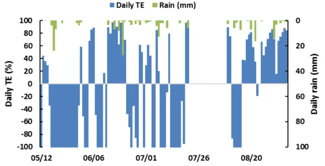
Figure 5 shows daily TE (estimated from turbidity measurements) and rainfall; gaps correspond to periods of outliers or absence of recorded data due to battery failure. At the beginning of the season, Basin A showed a positive efficiency that was minimally affected by rainfall, whereas from 06 July to 16 September it showed a negative efficiency for periods of low rainfall with Q ≤ 0.020 m³ s-1 _(total

number of hourly flow measurements for this period was 1615, of which 1453 were below 0.020 m³ s-1_).

During this period, SS downstream of the basin (as estimated from the turbidimeter data) was greater than SS upstream. This was also observed in 2016 (data not shown) and could be due to the growth of microscopic algae during the dry season affecting the turbidity recorded downstream of the basin. This hypothesis may explain why, according to the turbidity measurements, the basin does not seem to be efficient during periods of low flow, but a thorough study would be required to confirm.

For the 99-day time series, the accumulated SS loads upstream and downstream of Basin A were 48.0 and 37.7 metric ton respectively, giving a global mean TE of 21.6 % for the whole season. The trapping efficiency of Basin A was also computed for different classes of flow rate (Table 2). As shown in Table 2 and discussed earlier, the trapping efficiency for discharges lower than 0.020 m3 _s-1 _{was negative}

according to the SS concentrations estimated from the turbidimeter data.

ForPeatlandB,theaverageSSconcentrationswere 267.1 mg L-1 _{(standard deviation = 463.7 mg L}-1_;

Figure 5. Daily trapping efficiency TE (%) and daily rainfall for Basin A.

Table 2. TE (%) of Basin A and Basins B1–B2 calculated using data from the turbidimeters for the period May–September 2017.

Basin A Basins B1–B2

Flow class TE (%) Flow class TE (%)

Q ≤ 0.016 m³ s-1 _-139.6 Q ≤ 0.0032 m³ s-1 _80.9

0.016 < Q ≤ 0.020 m³ s-1 _-123.4 0.0032 < Q ≤ 0.0035 m³ s-1 _49.5

0.020 < Q ≤ 0.029 m³ s-1 _40.0 0.0035 < Q ≤ 0.0041 m³ s-1 _19.8

N=9132) upstream of Basin B1 and 71.4 mg L-1

downstream of Basin B2 (standard deviation=82.2 mg L-1_{; N=9132).}

Due to a malfunction of the turbidimeter in the channel that connects Basin B1 to Basin B2, it was not possible to calculate TE for B1 and B2 separately, so it was calculated only for B1 and B2 in series. As shown in Figure 6, the trapping efficiency of Basins B1–B2 declined to negative values after a rainy episode, meaning that high flows can lead to the resuspension of previously deposited SS.

Seasonal TE for Basins B1–B2 was computed from observed data over 95 days (from May to September). Cumulative loads for this period were 8.2 and 4.53 metric tons, respectively, upstream of B1 and downstream of B2. Seasonal TE for B1–B2 was, thus, 44.7 %.

As shown in Table 2, the trapping efficiency of Basins B1–B2 largely depends on flow rate. For Q≤0.0032 m³ s-1_{, when the flow rate was less than}

the average Q for the season (Q average = 0.00379 m³ s-1_{), TE was 80.9 % and decreased when the flow}

rate increased. However, TE computed from

turbidimeter data was lower for the third class of flow than for the fourth class. This was not expected since TE generally decreases when the flow rate increases; due to the increase in flow velocity, which reduces SS deposition and promotes re-suspension of settled particles.

Hydraulic modelling results

The Manning coefficient (n) values generated to calibrate the hydraulic models for Basins A, B1, and B2 are given in Table 3. For each model, n is greater in the basin than in the channels (except the channel connecting B1 and B2) owing to accumulation in the basin of mud and debris, which increases its roughness. Also, Manning’s values can be high in uncleaned basins (Haahti et al. 2017). Calibration of the hydraulic model of Basins B1 and B2 in series was not possible unless the Manning coefficient for the channel connecting B1 to B2 (output channel for B1, input for B2) was increased to unrealistic values. During the field season it was observed that the banks of this channel were unstable and continuously eroding, thus filling the channel with sediment, tree

Figure 6. Daily TE (%) and daily rainfall for basins B1–B2 in series.

Table 3. Manning roughness coefficients for 1 D hydraulic models of the studied basins. Manning roughness coefficient n Friction slope Sf

Basin A Basin B1 Basin B2 Basin A Basin B1 Basin B2 Input channel 0.099 0.150 0.450 - 0.00015 0.00015

Basin 0.150 0.300 0.300 - - -

branches and debris. This may explain why n in the channel exceeded n in Basins B1 and B2 and why the turbidimeter installed in this channel recorded outlier data.

The results of calibration and validation are given in Table 4, while simulated and observed water levels in the studied basins are illustrated in Figures 7–9.

Figure 7 shows that the calibrated hydraulic model of Basin A underestimated water levels downstream of the basin for low flows (Q < 0.0187 m³ s-1_{); the NSE}

and RMSE being, respectively, 0.95 and 0.059. For Q > 0.0468 m³ s-1 _{(corresponding to periods of heavy}

rainfall), the hydraulic model of Basin A over-estimated water levels upstream and downstream of

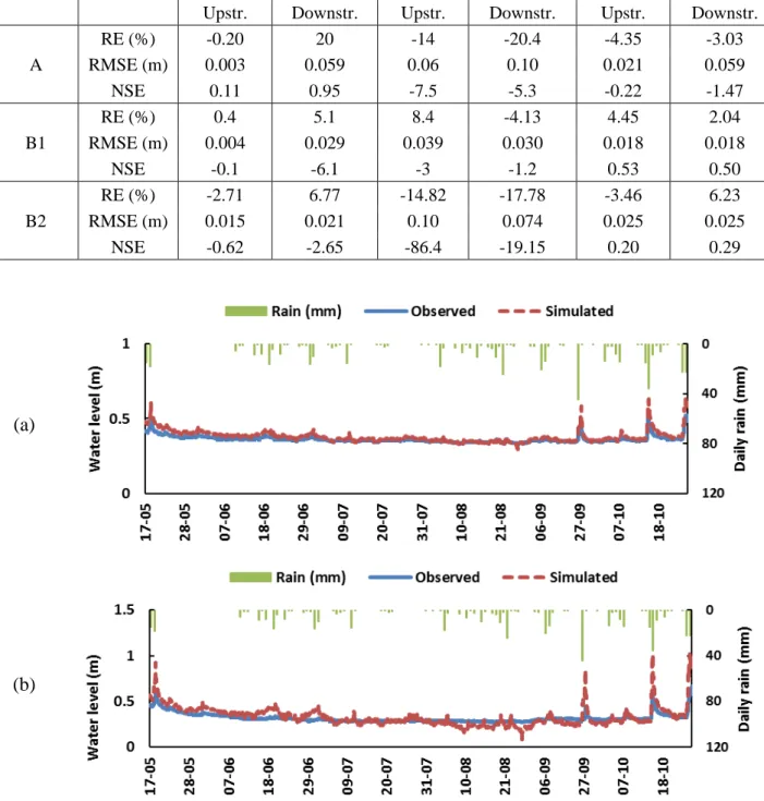
Table 4. Calibration and validation results of the hydraulic model for Basin A and Basins B1–B2 (in series).

Basin Criteria

Calibration Validation

Low Q High Q All flows

Upstr. Downstr. Upstr. Downstr. Upstr. Downstr. A RE (%) -0.20 20 -14 -20.4 -4.35 -3.03 RMSE (m) 0.003 0.059 0.06 0.10 0.021 0.059 NSE 0.11 0.95 -7.5 -5.3 -0.22 -1.47 B1 RE (%) 0.4 5.1 8.4 -4.13 4.45 2.04 RMSE (m) 0.004 0.029 0.039 0.030 0.018 0.018 NSE -0.1 -6.1 -3 -1.2 0.53 0.50 B2 RE (%) -2.71 6.77 -14.82 -17.78 -3.46 6.23 RMSE (m) 0.015 0.021 0.10 0.074 0.025 0.025 NSE -0.62 -2.65 -86.4 -19.15 0.20 0.29

(a)

(b)

Figure 7. Time series (hourly) of observed and simulated water levels (a) upstream and (b) downstream of Basin A.

(a)

(b)

Figure 8. Time series (hourly) of observed and simulated water levels (a) upstream and (b) downstream of Basin B1.

(a)

(b)

Figure 9. Time series (hourly) of observed and simulated water levels (a) upstream and (b) downstream of Basin B2.

the basin, which explains the negative NSE values. Relatively smooth recorded data, as shown in Figure 7a, could be explained by the fact that the water level gauge is not sensitive to small variations in water level (probe accuracy: standard error = ±0.075 %, 0.3 cm (0.01 ft); maximum error = ±0.15 %, 0.6 cm (0.02 ft)). There was no systematic bias in the entire simulated series of water levels; there was, rather, a seasonal bias that depended on flow variation in response to rainfall. For the entire season, the hydraulic model of Basin A better reproduced the simulated water levels upstream of the basin where NSE and RMSE were, respectively, -0.22 and 0.021, than downstream of the basin where NSE was -1.47 and RMSE was 0.059.

For Peatland B, the hydraulic models of Basins B1 and B2 were calibrated separately. As shown in Figure 8a, the hydraulic model of Basin B1 slightly underestimated water levels. For Basin B2, the hydraulic model over-estimated simulated water levels at flow rates higher than 0.00488 m3 _s-1

(frequency = 0.259) (Figure 9). In the case of Basin A, low NSE values (Table 4) arose because the model of Basin A over-estimated peak water levels, especially downstream of the basin (RE<0); however, as mentioned previously, this could be due to observed data errors. In Peatland B, on the other hand, the NSEs of the models for Basins B1, B2 and B1–B2 ranged from 0.20 to 0.53. Higher NSE values were attributable to the capacities of these models to generate the peak water levels corresponding to periods of intense flow.

Estimation of basin efficiency using the hydraulic and deposition models

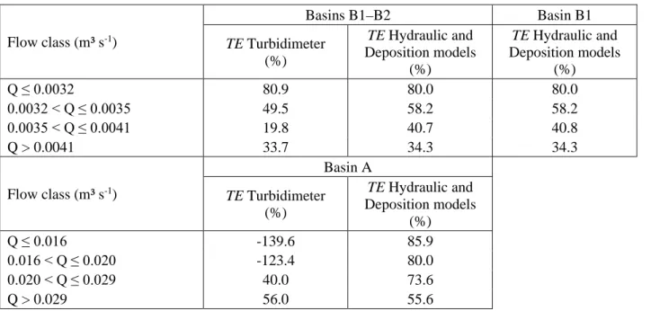
Trapping efficiencies for the studied basins, as calculated using turbidimeter data in conjunction with the hydraulic and deposition models, are given in Table 5. Due to irregularities in the turbidimeter data downstream of Basin B1 (as mentioned previously), TE was not computed individually for Basin B2 with the hydraulic and deposition models. For Basin A, TE estimated in this way ranged from 55.6 % for periods when Q > 0.029 m³ s-1 _{to 85.9 %}

for periods when Q < 0.016 m³ s-1_{. Similar results}

were obtained for Basins B1–B2 in series, with TE = 80 % for low flow rates (Q < 0.0032) and TE = 34.3 % for Q > 0.0041 m³ s-1 _{(Table 5). The TE}

values for Basin B1 alone and Basins B1–B2 in series were almost equal, meaning that particles which do not settle in Basin B1 will remain in suspension whilst travelling through Basin B2. For the third class of flow (0.0035 m³ s-1< Q ≤ 0.0041 m³ s-1_{), TE was}

slightly greater for Basin B1 than for Basins B1–B2. The lower TE of Basins B1–B2 was probably due to a re-suspension of particles in Basin B2.

Turbidimeter data collected in 2018, not presented here, show that the sediment load between Basin B1 and Basin B2 was less than the sediment load upstream of Basin B1, which suggests that Basin B1 is efficient in retaining SS.

In Peatland B, we focused on Basin B1 when evaluating the efficiency of flow and sediment control structures. The results of this evaluation (Table 6) show that the geotextile fabric and double

Table 5. Trapping efficiency (TE) of Basins B1–B2 in series, Basin B1 and Basin A, calculated using SS concentrations and the hydraulic and deposition models.

Flow class (m³ s-1₎ Basins B1–B2 Basin B1 TE Turbidimeter (%) TE Hydraulic and Deposition models (%) TE Hydraulic and Deposition models (%) Q ≤ 0.0032 80.9 80.0 80.0 0.0032 < Q ≤ 0.0035 49.5 58.2 58.2 0.0035 < Q ≤ 0.0041 19.8 40.7 40.8 Q > 0.0041 33.7 34.3 34.3 Flow class (m³ s-1₎ Basin A TE Turbidimeter (%) TE Hydraulic and Deposition models (%) Q ≤ 0.016 -139.6 85.9 0.016 < Q ≤ 0.020 -123.4 80.0 0.020 < Q ≤ 0.029 40.0 73.6 Q > 0.029 56.0 55.6

pipe culvert do not have a significant effect on the trapping efficiency of Basin B1, according to the results of the hydraulic and deposition models. This can be explained by the fact that the geotextile fabric only slightly reduces flow velocity in the basin. Its main function is to act as a barrier against coarse particles. However, since this barrier is located 42.8 m downstream of the entrance to Basin B1 it does not have any effect on TE because, according to the model results, the coarser particles are deposited at a maximum distance of 31.5 m downstream of the entrance to the basin. However, for periods with heavy rainfall events, flow will be more important, the fraction of coarser particles will increase and, therefore, the geotextile fabric will be especially necessary to retain coarse particles in short basins, where retention times are lower.

For the configuration of Basin B1 without a weir, the results (Table 6) illustrate the role of the weir in reducing flow velocity and allowing more SS to settle, especially when the flow is below 0.0035 m³ s- 1_{. This is in accordance with the results of Klove}

(2000), who showed that peak discharge control measures had a positive effect on the removal of suspended sediments at a peat extraction site in Finland.

DISCUSSION

The estimation of SS from turbidity measurements in environments such as cutover peatlands is not straightforward, and a few difficulties were encountered during the project. The main problems are listed below:

1. As stated above, continuously increasing turbidity measurements during the driest and warmer weeks of the summer at the downstream end of Basin A could be due to the growth of microscopic algae; this was also observed by Stenberg et al. (2015) in

a peatland in Finland, where high turbidity values were said to be caused by the growth of algae on the sensor.

2. Even if the hydro brush cleaned the turbidity sensor every 30 minutes, some debris (e.g. leaves) could get stuck on the sensor between brush movements and thus cause unrealistically high turbidity measurements.

3. In some cases (more frequent in the channel between Basins B1 and B2), abnormally high and fluctuating turbidity values could be due to the turbidimeter becoming partially submerged in the unconsolidated peat deposited on the bottom of the channel.

4. The relationship between turbidity and SS depends on the natural grain size distribution of suspended particles; SS estimates from calibration curves established using sediments collected at the bottom of the channel do not take into account the finest SS fractions.

Nonetheless, the observed concentrations of suspended sediments were of similar magnitude to those reported in previous studies. For example, Clément et al. (2009) observed some values higher than 200 mg L-1 _{downstream of a peat sedimentation}

basin. In the snowmelt period (April to May), St-Hilaire et al. (2006) observed that a concentration of 500 mg L-1 _{was exceeded between 11 % and 60 % of}

the time downstream of two extracted peatlands in Canada. Garneau et al. (2019) noted concentrations as high as 2500 mg L-1 _{downstream of a}

sedimentation basin during a rainfall event.

The observed daily and seasonal TE values for Basins A and B1–B2 were also similar to those computed in previous studies. Samson-Dô & St-Hilaire (2018) observed some negative daily TE values in seven basins located in the same regions, along with seasonal TE varying from less than -100 % to 85 %. Again in the same regions,

Table 6. TE of different configurations of Basin B1.

Flow class (m³/s) B1 B1 without geotextile curtain B1 with weir, without double pipe culvert B1 with weir, without geotextile and culvert B1 without weir Q ≤ 0.0032 80.0 80.0 80.0 80.0 56.0 0.0032 < Q ≤ 0.0035 58.2 58.2 58.2 58.2 41.0 0.0035 < Q ≤ 0.0041 40.8 40.8 40.8 40.8 40.0 Q > 0.0041 34.3 34.1 34.2 34.1 33.1

Garneau et al. (2019) computed seasonal TE varying from 29 % to 91 % for six basins, while Klove (2000) measured TE at 41 % and 68 % for peat sedimentation in Finland. By computing the 1–3 year average TE for 37 peat forestry sedimentation basins in Finland, Joensuu (1999) found that only half of the basins reduced the concentration of suspended solids. Also, we should remember that the seasonal TE computed here for Basins A (22 %) and B1–B2 (45 %) relate to the frost-free season only, since the sites were not accessible during the snowmelt period. If the snowmelt period had been monitored, lower seasonal TE could be expected since snowmelt is known to contribute significantly to annual suspended sediment yields from drained peatlands (Haahti et al. 2016).

Sources of uncertainty

Some uncertainties arise in relation to the rating curves. In Peatland B, where channels have been dug into the peat, the determination of depth using a graduated ruler was approximate and varied between operators. Due to this constraint, the elaboration of rating curves was challenging, especially in the case of the upstream curve for Basins B1–B2. Some points, mainly representing high flows, were eliminated because they seemed to be out of line. In addition, velocity measurements during periods of low flow were sometimes close to zero, which made flow estimation very difficult and affected the accuracy of the rating curves. It is important to note these difficulties because the flow series were used in the calculations of trapping efficiency (Equation 4) of basins using suspended sediments loads (Equation 5) and also to calibrate and validate the hydraulic models.

The Pavey et al. (2007) protocol employed for the calibration of turbidimeters may also be a potential source of uncertainty. Sediments used for the calibration process were collected from the bottom of the channel and were coarser than suspended particles, meaning that the calibration curves over-estimated suspended sediment concentrations. However, this uncertainty applied to the estimation of SS concentrations upstream and downstream of each studied basin, and would thus have minimal effect on the estimates of trapping efficiency. Difficulties associated with the estimation of SS from turbidity measurements in environments such as extracted peatlands, already detailed above, also add some uncertainty.

Concerning the hydraulic modelling, the field measurements of geometric data for the studied basins, and especially the depth measurements, present a source of errors. Because the depth

measurements were made during a period when the basins were filled with water, the depths of sections in the middles of the basins were estimated. Depth measurements were particularly difficult at Peatland B, where the basins were not riprapped. The measurements obtained also varied from one operator to another. In the hydraulic models elaborated, there were two calibration parameters (friction slope Sf and the Manning roughness coefficient n), which may add uncertainty since it is much easier to calibrate a model with one parameter than with two. In addition, using measurements obtained in the same year for both calibration and validation of the model can affect its reliability. For better model accuracy, testing with measurements from a different year is recommended.

Finally, the deposition model that we used to calculate the trapping efficiency of the studied basins involved some simplifications, in that all particle classes were assumed to represent the same percentage (10 %) of the sediment, and the settling velocity of the different classes were determined by calibration such that TE calculated by the model would be close to values calculated using the turbidimeter data. The settling velocities represent a significant source of error in the deposition model and would be better determined by laboratory tests. Also, accuracy could be improved by determining the percentages of different particle classes as a function of flow rates. Another simplification of the deposition model that may have led to under-estimation of settling velocity was that basin depth was assumed to remain constant throughout the season, without considering its variation as the particles settled. This simplification could cause major errors because basin depth can vary significantly during a season. For example, Clément et al. (2009) measured an accumulation of peat amounting to about 58 % of pond volume in a peat sedimentation basin only 64 days after pond maintenance. In the deposition model, the possibility that suspended particles may form colloids, which increases their settling velocity, was also not considered. Moreover, the simulated flow velocities used in the deposition model were probably under-estimated, and this can lead to over-estimation of the trapping efficiency of the basins. Lastly, the use of a two-dimensional hydraulic model could have provided better estimates of water velocities for the deposition model, especially in the vicinity of the flow control structures (culvert and weir).

Outcomes

The main objective of this article was to determine the trapping efficiency of three sedimentation basins

in two different peatlands using hydraulic and deposition models. The effectiveness of sedimentation basins in their role of retaining suspended sediments depends on several factors. Our results showed that the efficiency of the studied basins is highly dependent on flow, and that the introduction of some flow control structures could improve trapping efficiency. Among these, the installation of geotextile fabric presents a physical barrier to coarse sediments which will be beneficial (i.e. increase seasonal TE) only in short basins, since the coarser particles that can be retained by geotextile fabric would be trapped by longer basins even in the absence of this control structure. However, the geotextile fabric is necessary for periods of high flow where the coarser fraction of SS is significant and the retention time in the basin decreases. The double culvert results in only a slight increase of TE compared to a simple elevation in the bottom level of the basin (such as a weir) at its downstream end, but the presence of the double culvert is still important for the evacuation of floods with low recurrence. The presence of a weir at the outlet of the basin is, however, crucial to ensure high TE. Indeed, tests performed with the hydraulic and deposition models showed the importance of this control structure in reducing flow velocity and thus promoting suspended sediment deposition in the basin.

This work showed how the combined use of hydraulic and deposition models can help in assessing the effects of various basin configurations on TE, in order to find the configuration that is most efficient in maximising suspended sediment deposition. With a series of discharge inflows and knowing the settling velocities of suspended particles, a hydraulic model such as HEC-RAS and the deposition model we developed can be used together to compute TE for different basin configurations by varying width, length and/or depth of the basin and adding different control structures such as weirs, flow regulators, etc. The series of inflows could be provided either by measurements or by hydrological simulations. As for the settling velocities, they could be obtained experimentally or by calibration of the deposition model from observed SS series.

It should be noted, however, that the results presented here were obtained with a simplified deposition model, which assumes that the suspended solids entering the basins keep the same distribution of settling velocities regardless of the hydrological conditions. Further research and effort would be required to determine the distribution of settling velocities of suspended solids entering the basins in each peatland studied, during low flow and high flow

periods as well as during and after maintenance interventions. Moreover, in future work, resuspension of SS deposited in the basins should be integrated into the simulation model, since recent work has shown that this process can happen more frequently that initially suspected in some basins; more specifically at the downstream ends of long basins.

In hydraulic modelling of basins, taking into account the hydrodynamics of flow would allow a more reliable estimation of the amounts of suspended sediment exported and retained. These results can be transposed to sedimentation basins designed to minimise the discharged SS loads of any other type of water (wastewater, mining industry water, etc.).

This research determined the trapping efficiency of existing basins and the importance of the weir downstream in the retention of suspended sediment. The research also made it possible to find the basin configuration that would allow maximum retention of suspended sediment. It can be concluded from this study that the use of a single properly designed basin, with a weir at its downstream end, is sufficient to settle the coarser portion of the SS load. If it is necessary to retain finer particles, the sedimentation basin could be used in conjunction with an additional infrastructure such as a constructed wetland.

ACKNOWLEDGEMENTS

The authors thank the peat enterprises and APTHQ (Québec Horticultural Peat Moss Producers Association) for granting the research team access to their sedimentation basins and supporting this project; and FRQNT for financial support.

AUTHOR CONTRIBUTIONS

SH supervised and carried out fieldwork; performed data processing, calculations, calibration and validation of hydraulic models; and wrote the first version of the paper. SD and AS-H developed the methodology, participated in the field campaigns, verified the results and reviewed the paper.

REFERENCES

Benyahya, L., St-Hilaire, A., Courtenay, S.C., Boghen, A.D., Ouarda, T.B., Bobée, B., Lachance, M. (2003) Analyse de l’efficaité des bassin de sédimentation d’une tourbière exploitée : étude de cas de la plaine de St-Charles,

Nouveau-Brunswick (Efficiency Analysis of the Sedimentation Basins of a Harvested Peat Bog: Case Study of the St-Charles Plain, New Brunswick). Report R-686, INRS-ETE, Quebec, Canada, 38 pp. (in French).

Brown, C.B. (1943) Discussion of sedimentation in reservoirs. Proceedings of the American Society of Civil Engineers, 69, 1493−500.

Brune, G.M. (1953) Trap efficiency of reservoirs. Eos - Transactions American Geophysical Union, 34(3), 407−418. doi:10.1029/TR034i003p00407. Brunner, G.W. (2016) HEC-RAS River Analysis

System Hydraulic Reference Manual, Version 5.0. US Army Corps of Engineers, Davis, CA. 538 pp. Clément, M., St-Hilaire, A., Caissie, D., Chiasson, A., Courtenay, S., Hardie, P. (2009) An evaluation of mitigation measures to reduce impacts of peat harvesting on the aquatic habitat of the East Branch Portage river, New Brunswick, Canada. Canadian Water Resources Journal, 34(4), 441−452. doi:10.4296/cwrj3404441.

Cris, R., Buckmaster, S., Bain, C., Reed, M. (2014) Global Peatland Restoration: Demonstrating Success. IUCN UK National Committee Peatland Programme, Edinburgh, 64 pp.

Daigle, J.-Y., Gautreau-Daigle, H. (2001) Canadian Peat Harvesting and the Environment, Second Edition. Sustaining Wetlands Issues Paper No. 2001-1, North American Wetlands Conservation Council Committee, Ottawa, 41 pp.

Garneau, C., Duchesne, S., St-Hilaire, A. (2019) Comparison of modelling approaches to estimate trapping efficiency of sedimentation basins on peatlands used for peat extraction. Ecological Engineering, 133, 60−68. doi:10.1016/j.ecoleng. 2019.04.025.

Haahti, K., Marttila, H., Warsta, L., Kokkonen, T., Finer, L., Koivusalo, H. (2016) Modeling sediment transport after ditch network maintenance of a forested peatland. Water Resources Research, 52, 9001−9019. doi:10.1002/2016WR019442.

Haahti, K., Nieminen, M., Finér, L., Marttila, H., Kokkonen, T., Leinonen, A., Koivusalo, H. (2017) Model-based evaluation of sediment control in a drained peatland forest after ditch network maintenance. Canadian Journal of Forest Research, 48, 130−140. doi:10.1139/cjfr-2017-0269.

Heinemarm, H. (1981) A new sediment trap efficiency curve for small reservoirs. Journal of the American Water Resources Association, 17(5), 825−830. doi:10.1111/j.1752-1688.1981. tb01304.x.

Joensuu, S., Ahti, E., Vuollekoski, M. (1999) The

effects of peatland forest ditch maintenance on suspended solids in runoff. Boreal Environment Research, 4, 343-355.

Klove, B. (2000) Retention of suspended solids and sediment bound nutrients from peat harvesting sites with peak runoff control, constructed floodplains and sedimentation ponds. Boreal Environment Research, 5(1), 81−94.

Laine, A. (2001) Effects of peatland drainage on the size and diet of yearling salmon in a humic northern river. Archiv für Hydrobiologie, 151(1), 83−99. doi:10.1127/archiv-hydrobiol/151/2001/ 83.

Landry, J., Rochefort, L. (2011) Le drainage des tourbières: impacts et techniques de remouillage (Drainage of Peatlands: Impacts and Rewetting Techniques). Groupe de recherche en écologie des tourbières (Peatland Ecology Research Group), Laval University, Quebec, 53 pp. (in French). Marttila, H., Kløve, B. (2008) Erosion and delivery

of deposited peat sediment. Water Resources Research, 44(6), W06406, 10 pp. doi:10.1029/ 2007WR006486.

Nash, J.E., Sutcliffe, J.V. (1970) River flow forecasting through conceptual models part I - A discussion of principles. Journal of Hydrology, 10, 282−290. doi:10.1016/0022-1694(70)90255-6.

Paavilainen, E., Päivänen, J. (1995) Peatland Forestry: Ecology and Principles. Ecological Studies 111, Springer-Verlag, New York, 250 pp. Pavey, B., Saint-Hilaire, A., Courtenay, S., Ouarda, T., Bobée, B. (2007) Exploratory study of suspended sediment concentrations downstream of harvested peat bogs. Environmental Monitoring and Assessment, 135(1-3), 369−382. doi:10.1007/s10661-007-9656-8.

Samson-Dô, M., St-Hilaire, A. (2018) Characterizing and modelling the trapping efficiency of sedimentation basins downstream of harvested peat bog. Canadian Journal of Civil Engineering, 45, 478−488. doi:10.1139/cjce-2017-0330.

Schofield, K.A., Pringle, C.M., Meyer, J.L. (2004) Effects of increased bedload on algal‐and detrital‐ based stream food webs: Experimental manipulation of sediment and macroconsumers. Limnology and Oceanography, 49, 900−909. doi:10.4319/lo.2004.49.4.0900.

Stanek, W., Silc, T. (1977) Comparisons of four methods for determination of degree of peat humification (decomposition) with emphasis on the von Post method. Canadian Journal of Soil Science, 57(2), 109−117. doi:10.4141/cjss77-015. Stenberg, L., Tuukkanen, T., Finér, L., Marttila, H.,

Piirainen, S., Kløve, B., Koivusalo, H. (2015) Ditch erosion processes and sediment transport in a drained peatland forest. Ecological Engineering, 75, 421−433.

St-Hilaire, A., Courtenay, S.C., Diaz-Delgado, C., Pavey, B., Ouarda, T., Boghen, A., Bobee, B. (2006) Suspended sediment concentrations downstream of a harvested peat bog: Analysis and preliminary modelling of exceedances using logistic regression. Canadian Water Resources Journal, 31(3), 139−156. doi:10.4296/cwrj3103139.

Trimble, S.W., Bube, P. (1990) Improved reservoir trap efficiency prediction. The Environmental

Professional, 12, 255−272.

Verstraeten, G., Poesen, J. (2000) Estimating trap efficiency of small reservoirs and ponds: methods and implications for the assessment of sediment yield. Progress in Physical Geography, 24, 219−251. doi:10.1177/030913330002400204. Vuori, K.-M., Joensuu, I. (1996) Impact of forest

drainage on the macroinvertebrates of a small boreal headwater stream: do buffer zones protect lotic biodiversity? Biological Conservation, 77, 87−95. doi:10.1016/0006-3207(95)00123-9. Submitted 05 May 2019, final revision 18 Nov 2019 Editor: Jonathan Price

_______________________________________________________________________________________ Author for correspondence:

Professor Sophie Duchesne, INRS-ETE, 490 de la Couronne, Quebec City, G1K 9A9, Canada 418-654-3776. E-mail: sophie.duchesne@ete.inrs.ca

Appendix

Table A1. For each studied basin: dates of the start and end of the recording period, length and width, drained areas, sediment/flow control structures and the position, calibration and rating equation used to calculate, respectively, suspended sediment concentration (SS; mg L-1_{) and flow (Q; m}3 _s-1_{). V: turbidimeter signal (volt);}

H: water level (m). Basin Installed Removed DD/MM/YY Length Width (means) Drained area Control structures Positions of

control structures Calibration * R² Rating R²

A 17 /05/17 26/10/17

97.5 m

11.7 m 66 ha weir outlet of basin

Upstream SS = 655.29 V - 17.34 SS = 165.43 V - 18.95 Downstream SS = 10288 V - 77.08 SS = 2550 V - 57.17 0.98 0.98 0.97 0.97 Q = 3.97 H² - 2.13 H + 0.28 Q = 1.21 H² - 0.69 H + 0.13 0.98 0.87 B1 11/05/17 03/11/17 60.8 m 5.2 m 23 ha geotextile curtain double pipe culvert and weir

42.45 m from entrance of basin 65.32 m from entrance of basin Upstream SS = 542.96 - 97.06 SS = 2179.3 V - 107.56 Downstream SS = 35236 V² + 4252 V - 4.63 SS = 2234.6 V² + 1052.2 V + 3.76 0.98 0.98 0.99 0.99 Q = 0.017 H 1.61 Q = 0.076 H 5.56 0.23 0.97 B2 11/05/17 03/11/17 92.0 m 5.5 m geotextile curtain weir 30 m from entrance of basin outlet of basin Downstream SS = 569.42 V - 22.08 SS = 142.54 V - 22.83 0.98 0.98 Q = 0.76 H² - 0.35 H + 0.042 0.96 * If V < 2.5 volts, the first equation is used (low signal); and if V ≥ 2.5 volts, the second equation is used (high signal).

Figure A1. An example of a calibration curve: upstream of Basin B2 (for high range of voltage). Points correspond to the samples collected during the calibration process

Figure A2. An example of rating curve: upstream of Basin A. Points correspond to spot flow measurements taken during the field season.