Modeling of viscoelastic sandwich beams using solid-shell finite elements

Science Arts & Métiers (SAM)

is an open access repository that collects the work of Arts et Métiers Institute of Technology researchers and makes it freely available over the web where possible.

This is an author-deposited version published in: https://sam.ensam.eu

Handle ID: .http://hdl.handle.net/10985/10266

To cite this version :

Fessal KPEKY, Hakim BOUDAOUD, Farid ABED-MERAIM, El Mostafa DAYA - Modeling of viscoelastic sandwich beams using solid-shell finite elements - Composite Structures - Vol. 133, p.105-116 - 2015

Science Arts & Métiers (SAM)

is an open access repository that collects the work of Arts et Métiers ParisTech researchers and makes it freely available over the web where possible.

This is an author-deposited version published in: http://sam.ensam.eu

Handle ID: .http://hdl.handle.net/null

To cite this version :

Fessal KPEKY, Hakim BOUDAOUD, Farid ABED-MERAIM, El Mostafa DAYA - Modeling of viscoelastic sandwich beams using solid-shell finite elements - Modeling of viscoelastic sandwich beams using solid-shell finite elements - Vol. 133, p.105-116 - 2015

Modeling of viscoelastic sandwich beams using

solid–shell finite elements

Fessal Kpeky,a Hakim Boudaoud,a Farid Abed-Meraim,b,c* and El Mostafa Dayaa,c a _{Laboratoire d’Étude des Microstrutures et de Mécanique des Matériaux (LEM3), UMR CNRS 7239, Université de}

Lorraine, Ile du Saulcy Metz Cedex 01, France

b _{Laboratoire d’Étude des Microstrutures et de Mécanique des Matériaux (LEM3), UMR CNRS 7239, Arts et Métiers}

ParisTech, 4 rue A. Fresnel, 57078 Metz Cedex 03, France

c _{Laboratory of Excellence on Design of Alloy Metals for low-mAss Structures (DAMAS)}

ABSTRACT

The aim of this work is to propose vibration modeling of sandwich structures with soft core using solid–shell finite elements. Several approaches have been adopted in the literature to accurately model this type of structures; however, they show some limitations in certain configurations of high contrast of material properties or geometric aspect ratios between the different layers. In such situations, it is generally well-known that the use of higher-order or three-dimensional finite elements is more appropriate, but will generate a large number of degrees of freedom and, thereby, large CPU times. In this work, an alternative method is proposed by considering a recently developed linear hexahedral solid–shell element. This solid–shell element is implemented into Matlab in order to use the so-called solver Diamant, which couples Asymptotic Numerical Method (ANM) and Automatic Differentiation (AD). Numerical tests, including various cantilever sandwich beams as well as a simplified pattern of rail on sleepers, are performed to show the efficiency of the proposed approach.

Keywords:

Sandwich structures Vibration

Finite element analysis Solid–Shell

Computational modeling

1. Introduction

Problems involving vibration are encountered in many areas of mechanical, civil and aerospace engineering. In many cases, the vibrations are undesirable because they lead to noise and system dysfunction. To avoid these detrimental effects, an efficient passive solution to reduce vibrations, well-established for more than 50 years, consists in the use of sandwich structures with elastic faces and viscoelastic core [1,2,3], in which the damping is principally induced by the shear deformation of the core.

* Corresponding author. Tel.: +(33) 3.87.37.54.79; fax: +(33) 3.87.37.54.70.

The main numerical difficulties in modeling these structures lie first in the description of the kinematics to obtain reasonable computational costs, and secondly in the proper account of the shear of the core. This latter transverse shear is due to the difference in the in-plane displacements and to the contrast in stiffness between the different layers. In earlier contributions, models using classical laminate theories (CLT) have been developed based on the Kirchhoff–Love model. Then, various kinematic models and numerical methods have been developed to accurately determine the damping properties of viscoelastic sandwich structures under vibration. In this regard, Reissner [4] and Mindlin [5] established first order shear theories (FSDT) that take into account this shear deformation. However, the complete 3D formulation indicates that the shear deformation varies at least in a quadratic form through the thickness and the shear stress should be equal to zero on the outer surfaces of the skins. Subsequent studies, Reddy [6] and Touratier [7] (to name only these), have made major improvements by proposing higher-order shear theories (HSDT) of the displacement field in the thickness (cubic and sinusoidal, respectively). The main advantage of these approaches is to allow a parabolic description of the shear stress, while ensuring the condition of zero shear stress on the free surface of the sandwich structures. It should also be noted that, in the context of sandwich structures under vibration, a number of specific finite elements have been developed (see, e.g., [8–11]) in order to discretize various types of geometries (e.g., beams, shells, conical shells …).

However, in the former studies, the sandwich structure is modeled as a single layer to facilitate analysis with reasonable computational cost. Unfortunately, the discontinuity of physical/mechanical properties in the thickness direction makes inadequate those theories, which were originally developed for one-layered structures. In addition, such a framework does not allow correctly describing some phenomena in a structure exhibiting high contrast of stiffness between different layers. To compensate these shortcomings and restrictions, zigzag theories have been developed in the literature, with interlaminar continuity (IC-ZZT) or without (ID-ZZT). These theories describe layer-by-layer the displacement field ensuring continuity conditions of the displacement field imposed at the interfaces between the core and the faces. Carrera [12,13] has provided a very comprehensive and well-documented historical review on zigzag theories for multilayered plates and shells as well as on modeling of multilayered and composite structures. In recent years, the zigzag approach has been applied in the context of vibration analysis (see, e.g., Boudaoud et al. [14], Bilasse et al. [15], Abdoun et al. [16], as well as the more recent review and assessment of existing models by Hu et al. [17]). Another noteworthy approach consists of Carrera’s unified formulation (CUF) [18], in which several kinematic assumptions for the displacement fields can be included hierarchically in one single compact formulation.

Considering some limitations of the zigzag models that have been shown in [17], an alternative approach could be the use of three-dimensional finite element assemblies, but this generally leads to a large number of degrees of freedom. Another approach proposed in this work consists in the use of a solid–shell element based on a fully three-dimensional formulation. This solid–shell element has been developed in order to correctly take into account the through-thickness phenomena, while maintaining the CPU time at reasonable levels [19,20,21]. It consists of a linear isoparametric hexahedral element having only nodal displacements as degrees of freedom and

constitutive matrix was also modified in order to approach shell-like behavior. To control the zero-energy hourglass modes, due to the reduced integration, an effective stabilization technique was used following the “Assumed Strain” method proposed by Belytschko and Bindeman [22], which is also intended to eliminate the remaining locking phenomena. A set of selective and representative benchmark tests was analyzed to show the effectiveness of this solid–shell element in linear and nonlinear problems. More recently, Salahouelhadj et al. [23] successfully simulated sheet metal forming processes using the SHB8PS solid–shell element coupled with an anisotropic large strain elastic–plastic model.

From a numerical point of view, the frequency dependency of the viscoelastic layer leads to nonlinear vibration problems. Among the various methods proposed to solve such nonlinear vibration problems, some show a number of restrictions and limitations, such as the complex eigenvalue method [24,25], the modal strain energy analysis [26,27], the direct frequency response procedure [28], and the asymptotic approach [29], while the order-reduction-iteration technique [30] and the homotopy-based asymptotic numerical strategy [31,32] are of more general applicability. The latter asymptotic numerical method makes use of homotopy [33] and of perturbation technique [34] in its continuation procedure. Detailed discussions and reviews of the above-mentioned methods as well as of their multiple variants can be found in the literature (see, e.g., [31,32] and more recently [35]). The purpose of the current work is to combine the above-discussed solid–shell concept with sandwich structure modeling in order to evaluate the capabilities of the resulting formulation in analyzing vibration of sandwich structures.

The paper is organized as follows. Section 2 presents the general formulation of the problem using different finite element discretizations, while underlying their respective limitations. The formulation of the solid–shell finite element is described in Section 3. The solving method (the so-called solver Diamant), which couples Asymptotic Numerical Method (ANM) and Automatic Differentiation (AD), is briefly outlined in Section 4. The numerical tests are shown in Section 5, along with the associated discussions, and the main conclusions are drawn in Section 6.

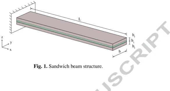
2. Formulation of the problem, different discretizations and their limitations In this work, we consider the free vibration problem of a sandwich beam schematized in Fig. 1. Different finite element discretizations will be adopted in order to compare their respective performance and to emphasize potential limitations. The basic equilibrium equations are obtained by using the virtual work principle as follows:

2 2 0 v d r _t d dv æ _{: +} ¶ _× ö ₌ ç _¶ ÷ è ø

ò

s e u u (1)

where s , e and u are, respectively, the stress and strain tensors, and the generalized

displacement at a point within the body v of the viscoelastic structure, while the density of the material is denoted by r. The stress and strain tensors s and e as well as the displacement u can be expressed as harmonic time functions.

Fig. 1. Sandwich beam structure.

The viscoelastic damping behavior is accounted for through the stress–strain law, which can be written in the form:

( )

w : =

s C e with _C

( )

w =_CR

( )

w +_iCI

( )

w

(2) where _CR

( )

w _{and C}I

( )

w _{are, respectively, the tensors characterizing the energy} storage and dissipative behavior of the viscoelastic material.

Combining Eqs. (1) and (2), and using a finite element discretization, the natural vibration problem of viscoelastic structures can be written in the following form:

( )

w w2

{ }

é - ù =

ëK Mû U 0 (3)

where M and K denote, respectively, the mass and stiffness matrix of the structure, and the complex nodal vibration eigenmode is denoted by U .

In Hu et al. [17], the limitations of the CLT, FSDT and HSDT models have been presented in details, while emphasizing the advantage of ZZT. However, the ZZT also has limitations related to high geometric ratios or contrast in material stiffness between the layers. To demonstrate this, simulation results of eigenfrequencies are given in what follows, which compare the IC-ZZT with quadratic 2D and 3D elements from Abaqus (CPE8R: 2D strain quadratic element with reduced integration, CPS8R: 2D plane-stress quadratic element with reduced integration, and C3D20R: 3D hexahedral quadratic element with reduced integration). The results obtained with the C3D20R element are taken as reference. This analysis is conducted on a simple cantilever beam.

Table 1

Sandwich beam parameters.

f E r_f r_c h nf nc 6.9x1010_{Pa 2766 kg.m}-3 _{1600 kg.m}-3 _{0.05 m 0.3 0.49} L b z y x h_c h_f h_f

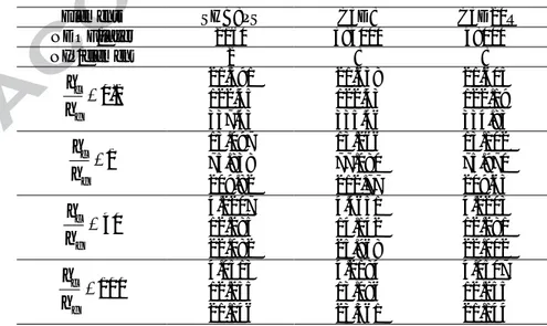
Table 2 Influence of Ec/Ef (hc/hf = 1, L/h = 20). C3D20R CPE8R CPS8R FSDT IC-ZZT 100 c f E E = 95.860 106.71 94.031 93.988 597.92 665.74 586.53 588.51 1664.5 1851.6 1630.7 1645.6 Table 3 Influence of L/h (hc/hf = 1, Ec/Ef = 10-5). C3D20R CPE8R CPS8R FSDT IC-ZZT 4 L h = 300.77 309.06 290.56 296.72 1750.3 1792.0 1995.4 1856.4 5559.1 5701.1 5394.2 5197.3 Table 4 Influence of hc/hf (L/h = 20, Ec/Ef = 10-5). C3D20R CPE8R CPS8R FSDT IC-ZZT 2 10 c f h h -= 31.212148.05 32.173153.10 31.088147.38 27.103136.66 377.50 391.52 375.50 365.87

The material and geometric properties of Table 1, combined with the material ratio (Ec/Ef) and the geometric ratios (L/h) and (hc/hf), are used. The first three eigenfrequencies are reported in Tables 2–4 and correspond to the converged meshes. These results show that the IC-ZZT is not suitable for the configurations associated with Tables 3 and 4, which confirms its restrictions in terms of range of applicability beyond certain limits. It is also clear from Tables 2–4 that the 2D formulation becomes less accurate because it does not take into account either the through-width effects, in the case of the plane-strain element CPE8R, or the through-thickness effects, in the case of the plane-stress element CPS8R.

The above simulation results highlight the limitations of such models devoted to viscoelastic sandwich structure modeling. To overcome these limitations, a new finite element method is developed coupling the solid–shell concept and the so-called Diamant approach. This alternative finite element strategy is presented in Section 3 below.

3. New finite element discretization of free vibration problems

Unlike the traditional literature models for sandwich structures, we propose in this work a new finite element method to discretize the problem in the form of Eq. (3), and to solve the latter for any geometric and material configuration of sandwich structures. To achieve this goal, the SHB8PS solid–shell element is considered. A short description

of this solid–shell formulation is provided in this section, the detailed derivation can be found in [19,20].

3.1. Kinematics and interpolation

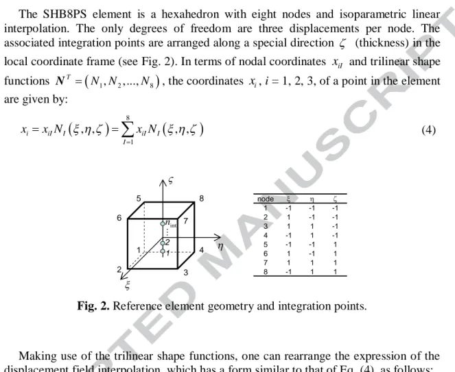
The SHB8PS element is a hexahedron with eight nodes and isoparametric linear interpolation. The only degrees of freedom are three displacements per node. The associated integration points are arranged along a special direction z (thickness) in the local coordinate frame (see Fig. 2). In terms of nodal coordinates x and trilinear shape_iI functions T

(

₁, ₂,..., ₈

)

N N N

=

N , the coordinates x , i = 1, 2, 3, of a point in the element_i are given by:

(

)

8

(

)

1 , , , , i iI I iI I I x x N x h z x N x h z = = =

å

(4)

Fig. 2. Reference element geometry and integration points.

Making use of the trilinear shape functions, one can rearrange the expression of the displacement field interpolation, which has a form similar to that of Eq. (4), as follows:

(

0 1 1 2 2 3 3 1 1 2 2 3 3 4 4

)

T T T T T T T i i i u = a +xb +x b +xb +hγ +h γ +hγ +h γ ×d (5) where ( )

(

)

, = = =0 1 2 3 4 3 1 , 1, 2, 3 , , , 1 , =1,..., 4 8 T j i i i j j i x h h h h a x h z a a hz zx xh xhz a = ¶ = = = ¶ = = = = = - å ì ï ïï í ï _{é ù} × ï _{ê ú} ë û ïî 0 γ N b N h h x b (6)

In Eqs. (5) and (6), vectors d and_i x , which indicate the nodal displacements and_i

coordinates, are defined as:

(

)

(

11 22 33 88

)

, , , ..., , , , ..., T i i i i i T i i i i i u u u u x x x x = = ìï í ïî d x (7) x h V 1 2 ₃ 4 5 6 ₇ 8 1 2 … node x h z 1 -1 -1 -1 2 1 -1 -1 3 1 1 -1 4 -1 1 -1 5 -1 -1 1 6 1 -1 1 7 1 1 1 8 -1 1 1 int n

Vectors h are given by:_a

(

)

(

)

(

)

(

)

1 2 3 4 1,1, 1, 1, 1, 1,1,1 1, 1, 1,1, 1,1,1, 1 1, 1,1, 1,1, 1,1, 1 1,1, 1,1,1, 1,1, 1 T T T T = = = = -- -- - -- - - -- - -

-ì

ï

ï

í

ï

ï

î

h h h h (8)

As mentioned before, this is an eight-node hexahedral element formulated on the basis of a fully three-dimensional approach. In other words, it has only displacement degrees of freedom and the same kinematics and interpolation as a classical three-dimensional linear solid element. However, specific changes have been made to avoid a number of numerical problems, namely hourglass-type instabilities and locking phenomena, and thereby to provide this solid–shell element with shell-like behavior. 3.2. Hourglass mode control and locking treatment

Using the Hu–Washizu variational principle in combination with the Assumed Strain Method (ASM) proposed by Belytschko and Bindeman [22], and considering the nonlinear frequency dependent material stiffness, the elementary stiffness matrix can be expressed as:

( )

ˆ

( )

ˆ e T e w =

ò

_V × w × dV K B C B ₍₉₎

where Bˆ denotes the projected discrete gradient operator, as modified by the Assumed Strain Method (see, e.g., [22]), which is defined by:

1 14 2 14 3 13 2 12 1 12 1 12 3 12 3 12 2 12 , , , ˆ ˆ ˆ ˆ ˆ ˆ ˆ _; ˆ ˆ ˆ ˆ ˆ ˆ ˆ ˆ ˆ ˆ ˆ ˆ ˆ _{ˆ ;} ˆ _{ˆ ;} ˆ _ˆ T T T T T T T T T T T T T T T T T T x y z h h h g g g bg a a bg a a bg a a a b= a b= a b= é ₊ ù ê ú + ê ú ê ú + ê ú = ê _{+ +} ú ê ú ê _{+ +} ú ê ú + + ê ú ë û =

å

=

å

=

å

0 ₀ 0 0 0 0 0 0 0 γ γ γ b X b Y b Z B b Y b X b X b Z b Z b Y X Y Z (10)

InEq. (10), the b_i vectors, originally defined by Hallquist (see Eq. (6)), are replaced by the mean form proposed in Flanagan and Belytschko [36]:

(

)

, 1 ˆ _{, , ; 1...3} e i _V i e dV i V x h z =

ò

= b N (11)

One of the main features of the SHB8PS element concerns its integration points, which are all located on a fiber corresponding to

(

x =0,h = 0

)

. This particularity, along with the associated special direction designated as the ‘thickness’, is specifically intended to provide the element with shell-like behavior. However, this in-plane reduced quadrature induces hourglass modes that require stabilization. Recall that the

hourglass modes are associated with displacement patterns that induce zero strains at the points where the strains are calculated. These spurious zero-energy modes are due to a difference of rank between the kernel of the continuous stiffness matrix and that of the discretized one. The analysis of kernel of the stiffness matrix [19,20] obtained by numerical integration reveals the presence of the following six hourglass modes:

3 4 3 4 3 4 , , , , , æ ö æ ö æ ö æ ö æ ö æ ö ç ÷ ç ÷ ç ÷ ç ÷ ç ÷ ç ÷ ç ÷ ç ÷ ç ÷ ç ÷ ç ÷ ç ÷ ç ÷ ç ÷ ç ÷ ç ÷ ç ÷ ç ÷ è ø è ø è ø è ø è ø è ø 0 0 0 0 0 0 0 0 0 0 0 0 h h h h h h (12)

The control of these hourglass modes is achieved by adding a stabilization stiffness matrix. This procedure will be summarized in the next section. In addition to the ASM aimed at removing shear and membrane locking, the elasticity constitutive matrix is also modified to enhance the element immunity with regard to thickness locking, and in order to approach shell-like behavior. This specific elasticity law adopted here is given by the following constitutive matrix:

( )

2 0 0 0 0 2 0 0 0 0 0 0 0 0 0 0 0 0 0 0 0 0 0 0 0 0 0 0 0 0 E l m l l l m w m m m é + ù ê ú + ê ú ê ú ê ú = ê ú ê ú ê ú ê ú ë û C with

( )

* 2 1 E w n l n = - and

( )

(

)

* 2 1 E w m n = + (13)

where E and* n are Young’s modulus and Poisson’s ratio.

This choice allows us to avoid the locking phenomena encountered with the fully three-dimensional constitutive matrix and, in contrast to a plane-stress constitutive law, to take into account the strain energy associated with the strains normal to the shell mid surface.

3.3. Stabilization matrix and co-rotational frame

As discussed above, six hourglass modes appear and need to be stabilized. To achieve this goal, the procedure proposed in [22] is used. This approach combines an efficient stabilization technique with an assumed strain method. To begin with, the Bˆ

operator is decomposed into the sum of two operators B andˆ₁₂ B :ˆ₃₄

1 12 34 2 12 34 3 3 12 12 34 2 12 1 12 1 12 ˆ ˆ ˆ ˆ ˆ ˆ ˆ ˆ ˆ ˆ _and ˆ ˆ ˆ ˆ ˆ ˆ ˆ ˆ ˆ T T T T T T T T T T T T T T T T T é ₊ ù _{é ù} ê ú _{ê ú} + ê ú _{ê ú} ê ú _{ê ú} + ê ú _{ê ú} =_{ê ú} = ê ú + + ê ú _{ê ú} ê _{+ +} ú _{ê ú} ê ú 0 0 0 0 0 0 0 0 0 0 0 0 0 0 0 0 0 0 0 0 b X X b Y Y Z b Z B B b Y b X b X b Z (14)

The stiffness matrix becomes then:

( )

12 12 12 34 34 12 34 34 ˆ ˆ ˆ ˆ ˆ ˆ ˆ ˆ e e e e T T e _{V V} T T V V dV dV dV dV w = × × + × × + × × + × ×

ò

ò

ò

ò

K B C B B C B B C B B C B (15)

One can show that B vanishes at all of the integration points of the SHB8PSˆ₃₄

element. Therefore, if the Bˆ operator is evaluated at this set of integration points, it reduces to B . In order to recover the correct stiffness matrix using only the set ofˆ₁₂

integration points given above, we can write:

( )

( )

( )

( )

( )

( )

( )

( )

( )

12 12 12 12 12 34 34 12 34 34 ˆ ˆ where ˆ ˆ and ˆ ˆ ˆ ˆ e e e e e Stab T V T Stab V T T V V dV dV dV dV w w w w w w w w w = + = × × = × × + × × + × ×

ò

ò

ò

ò

K K K K B C B K B C B B C B B C B (16)

The stabilization stiffness is evaluated in a co-rotational coordinate frame. The adopted orthogonal co-rotational system is defined by the rotation matrix R that maps a vector in the global coordinate system to the co-rotational one. The components of the first two column vectors of matrix R, denoted respectively a_1i and a_2i, are given by:

1 1 , 2 2 , 1, 2, 3 T T i i i i a =L ×x a =L ×x i = (17) where

(

)

(

)

1 2 1,1,1, 1, 1,1,1, 1 1, 1,1,1, 1, 1,1,1 T T ì = - - - -ï í = - - -ïî L L (18)

Then, the second column vector a₂ is modified in order to make it orthogonal to a₁. A correction vector a_c is added to a₂ such that:

(

)

1 2 1 2 1 1 1 0 T T c c T × × + = Þ = -× a a a a a a a a a (19)

The third base vector a₃ is finally obtained by the cross-product a₃ =a₁Ù

(

a₂+a_c

)

, which gives the components of the rotation matrix after normalization by:

1 2 3 1 2 3 1 2 3 , , , 1, 2, 3 i i ci i i i i c a a a a R = R = + R = i= + a a a a (20)

At this stage, the natural vibration problem of viscoelastic structures, established in Eq. (3), will be discretized using the solid–shell finite element developed above in order to be solved by the so-called Diamant method presented in Section 4.

4. Numerical resolution

In this section, the finite element technology proposed above is first applied to discretize the problem in the form of Eq. (3). Then, to solve the resulting complex nonlinear eigenvalue problem associated with Eq. (3), the so-called Diamant approach [37] is adopted. This method couples the Asymptotic Numerical Method (ANM) and the automatic differentiation (AD) technique, which allows automatically computing higher order derivatives. The main advantage of this kind of approach lies in the fact that the Diamant method can be used for any nonlinear viscoelastic model. More details regarding this approach can be found in [38–40]. A short outline of this method is described in the following lines.

First, one can write the stiffness matrix é_ëK

( )

w ù_û as follows:

( )

( )

( )

( )

( )

( )

( )

( )

* * * 0 0 0 0 E E E E E w w w w = + ì ï = í ï ₌ -î K K K K K (21)

The modulus of delayed elasticity E*

( )

0 is always real and, therefore, the elasticity matrix K

( )

0 is real symmetric and positive definite. The matrix K is constant. Accordingly, the natural vibration problem can be rewritten as:

( )

( )

2

{ }

0 E w w

é + - ù =

ëK K Mû U 0 (22)

Assuming that l w= 2

, the unknowns U and l are sought in the form:

0 0 ; 0 1 N j j j N j j j p p p l l = = ì ₌ ï ï _{£ £} í ï = ïî

å

å

U U (23)

in which p denotes the path parameter and N the truncation order.

Using Eq. (21), solving the free vibration problem (22) consists in a set of residual equations:

(

)

( )

( )

{ }

(

)

(

)

(

)

( )

{ }

(

)

( )

[ ]

{ }

, 0 , , , 0 , E E l w l l l l l l w =é_ë + - ù_û = + = =é_ë - ù_û = 0 R U K K M U S U T U S U K M U T U K U (24)

At this stage, the homotopy technique is introduced to drive the solution from the real eigenvalue problem S U

(

,l = 0

)

obtained from:

(

, ,l p

)

=

(

,l

)

+p

(

,l

)

= 0

R U S U T U (25)

when p=0 (and whose known solution corresponds to

(

U,l

) (

= U₀,l₀

)

), to the complex eigenvalue solution of the residual problem (24), which is associated with

1

p= . Through this process, the part of solution

(

U

( ) ( )

p ,l p

)

is computed by using Taylor series

(

S T_j, _j

)

of functions

(

S T,

)

and by solving:

( )

( )

1 1 1 1 | | 1 0 0 0 0 0 0 0 | , 0 | , 0 1 0 1| , 1 1| , 1 { } { } { } 0 ₀ where 0 { } { } { } { } { } j j j j j j j j j j T T j j j j _T p pE p p l l l l k l l l = = -= = = = -= = = = - - -ì ü é ù ì ü ï₌ ï í ý í ý ê ú ï ï î þ ë û _{î þ} = - + é ù ×_ë + + _û = -é ù ×_ë + _û 0 0 0 0 0 0 U U U U U U S T T A U U U A K M K U S T T U S T (26)

where k is the Lagrange multiplier.

The complete solution

(

U,l

)

is obtained with the continuation procedure proposed in [39]. This procedure allows computing the exact complex eigenmode U and eigenfrequency w , which is the square root of l. The associated linear frequency W_n and loss factorh_n at the nth rank can be obtained by:

(

)

2 2

1

n n n

w = W +h (27)

Finally, this method is used to implement a solver called Diamant in Matlab. Once this numerical tool implemented, to generate the solution of Eq. (3), the user only has to define the finite element matrices K

( )

0 , K , M , the starting guess

(

U₀,l₀

)

, the truncation order N and the desired precision.

In order to emphasize the benefits of the proposed modeling approach, some numerical applications are presented in Section 5 for validation purposes.

5. Numerical tests and discussions

To assess the ability of the present SHB8PS solid–shell element to model vibrations of multi-layer structures, various beam structures in different material and geometric configurations of sandwich contrast are first investigated. The results are compared to those given by some state-of-the-art finite elements available in the commercial software package Abaqus/Standard. The three-dimensional elements selected from Abaqus for comparison consist of the linear solid element C3D8 (eight nodes, full integration) and the quadratic solid element C3D20R (twenty nodes, reduced integration). The latter is supposed to be a reference in this study, which will also be confirmed later, because of its well-recognized performance in this type of problems.

Nevertheless, first of all and before we proceed further, the SHB8PS solid–shell finite element will be first validated on a simple cantilever beam and on the sandwich beam problem studied in [15,16].

5.1. Validation tests

5.1.1 Simple cantilever beam

In this preliminary study, the natural frequencies are computed using the geometric and material properties reported in Table 5.

Table 5

Geometric and material properties of the simple cantilever beam.

E n ρ L h b

2.11x1011 _{Pa 0.3 7800 kg.m}-3 _{1 m 0.01 m 0.1 m}

The first four eigenfrequencies obtained with the proposed SHB8PS solid–shell and the classical solid linear element C3D8R (reduced integration), available in Abaqus, are compared with the analytical reference results and reported in Table 6. The calculations are performed for different mesh sizes, in which the number of elements is given in the following order: length x width x thickness. Note that only two integration points are used in the case of the SHB8PS solid–shell element.

It is clear from Table 6 that the SHB8PS solid–shell element outperforms the C3D8R in vibration modeling of a single layer beam. In the next section, a more selective and representative problem for the vibration modeling of viscoelastic sandwich structures will be investigated.

Table 6

Eigenfrequencies of the cantilever beam.

Element type Mesh layout f1 ref= 8.4 f2 ref = 52.5 f3 ref = 83.8 f4 ref = 147.1

f1/f1ref f2/f2ref f3/f3ref f4/f4ref

C3D8R (30x3x1)=90 0.10 0.10 0.18 0.20 (40x4x1)=160 0.10 0.10 0.18 0.20 (80x8x1)=640 0.10 0.10 0.18 0.19 (30x3x4)=360 0.94 0.97 0.94 0.97 (40x4x4)= 640 0.98 0.98 0.96 0.98 (80x8x4)=2560 0.98 0.98 0.99 0.99 (30x3x5)=450 0.98 0.99 0.94 0.99 (40x4x5)=800 0.99 0.99 0.96 1.00 (80x8x5)=3200 1.00 1.00 0.99 1.00 SHB8PS (30x3x1)=90 1.00 1.01 1.00 1.01 (40x4x1)=160 1.00 1.01 1.00 1.01

5.1.2 Viscoelastic sandwich beam

(respectively, C3D8 and C3D20R) are also used for comparison purposes. The geometric and material properties used in this study are reported in Table 7. The viscoelastic properties of the core are assumed to be constant and can be written as:

(

)

0 1

c c

E =E +ih (28)

where E₀ is the Young modulus of the delayed elasticity and h_c the core loss factor. The results corresponding to the first five modes are given in Table 8. Only the converged mesh for each finite element discretization is presented. These results not only validate the proposed solid–shell modeling approach, but also emphasize the advantage of the SHB8PS finite element, in particular in terms of coarse-mesh accuracy (compare the number of degrees of freedom (NDOF) as well as the number of integration points (NIP) required for each formulation, as reported in Table 8).

Table 7

Geometric and material properties of the viscoelastic sandwich beam.

Elastic faces Young’s modulus 10 6.9 10 P a f E = ´ Poisson’s ration =f 0.3 Density 3 2766 Kg m f r _{= ×} -Thickness hf =1.524 mm Viscoelastic core Young’s modulus 6 1.794 10 Pa c E = ´ Poisson’s rationc=0.3 Density 3 968.1 Kg m c r _{= ×} -Thickness hc =0.127 mm

Geometry of the beam Length L=177.8 mm

Width b=12.7 mm

Table 8

Frequencies and loss factors associated with the first five modes for the viscoelastic cantilever sandwich beam.

SHB8PS C3D8 C3D20R FSDT IC-ZZT [15] NDOF/layer 2160 384000 48000 3000 NIP/element 2 8 8 -(Hz) f h hc f(Hz) h hc f(Hz) h hc f(Hz) h hc 0.1 c h = 64.3 0.281 63.5 0.281 64.3 0.275 64.1 0.281 297.6 0.241 291.3 0.249 297.9 0.237 296.7 0.242 748.3 0.152 727.8 0.160 747.4 0.149 744.5 0.154 1405.3 0.087 1360.9 0.092 1400.7 0.086 1395.7 0.089 2278.1 0.056 2205.8 0.058 2272.5 0.055 2264.5 0.057

5.2 Contribution to modeling viscoelastic sandwich beams

The following analysis is specifically intended to show the effectiveness of this solid–shell element in modeling sandwich beams, especially beyond the restrictions

pointed out by Hu et al. [17]. In this investigation, the results obtained with the SHB8PS element are compared to those yielded by Abaqus formulations, which consist respectively of the C3D8 (3D hexahedral linear element with full integration) and the C3D20R (3D hexahedral quadratic element with reduced integration). The material and geometric properties for this viscoelastic sandwich beam problem are given in Table 9.

Table 9

Sandwich beam parameters.

f

E r_f r_c h nf nc

6.9x1010_{Pa 2766 kg.m}-3 _{1600 kg.m}-3 _{0.05 m 0.3 0.49}

The viscoelastic behavior of the core material is described, based on generalized Maxwell’s model, by:

( )

0 3 1 1 j c j j G G i w w w = æ D ö = ç_ç + ÷_÷ - W è

å

ø (29)

where G₀ is the shear modulus of the delayed elasticity, while the remaining parameters

(

D W are reported in Table 10._j, _j

)

Table 10

Maxwell’s series terms for the viscoelastic model.

j Dj 1 (rad.s ) j -W 1 0.746 468.7 2 3.265 4742.4 3 43.284 71532.5

Three dimensionless beam parameters are used in this comparative study, namely the ratio of core to face Young modulus (Ec/Ef), the ratio of beam length to beam total thickness (L/h), and the ratio of core to skin thickness (hc/hf). Let us remark that under these considerations and by using the material parameters as listed in Table 9, all sandwich beam possible configurations can be represented. For these purposes, frequencies and loss factors are evaluated in three configurations:

Case 1. Thin/thick core: 0.1£hc hf/ £100 (L h/ =20 ; Ec Ef/ = ´2 10-5) Case 2. Short/long beam: 4£L h/ £100 (hc hf/ =1 ; Ec Ef/ = ´2 10-5) Case 3. Soft/rigid core: 0.0001£Ec Ef/ £100 (hc hf/ =1 ; L h/ =20)

In order to assess the performance of the proposed finite element modeling, eigenfrequencies of sandwich beams in the above configurations have been investigated

previously (see Tables 2–4 in Section 2), all of the models discussed in the above section are investigated to evaluate their respective limits. For all of the configurations, a convergence study was first carried out and only the degrees of freedom (DOF) giving converged results are presented. The results corresponding to the first three eigenfrequencies are reported in Tables 11–13. The numbers indicated in bold reveal limitations associated with some models for certain values of the investigated dimensionless beam parameters. For such parameter ranges, these models do not provide accurate eigenfrequencies or require much finer meshes thus significantly increasing the number of DOF, which makes the analysis inefficient. One can observe that the results given by the SHB8PS are most often close to those yielded by the C3D20R, which can be considered as reference. However, the C3D20R requires a much larger number of DOF, which corresponds to a significantly higher computational effort. One can also notice that despite the large number of DOF required for the C3D8, its results are relatively poor and start deviating from the reference results as soon as the ratio h_c /h_f becomes greater than 1 (see Table 11). These limitations are mostly attributable to the high sensitivity of the C3D8 to locking phenomena, which overly stiffens the element and thus tends to overestimate the simulated eigenfrequencies.

A noteworthy observation from all of these sensitivity analyses (see Tables 11–13) is that the proposed solid–shell element formulation is able to provide accurate results for the different configurations investigated, while maintaining reasonable CPU times.

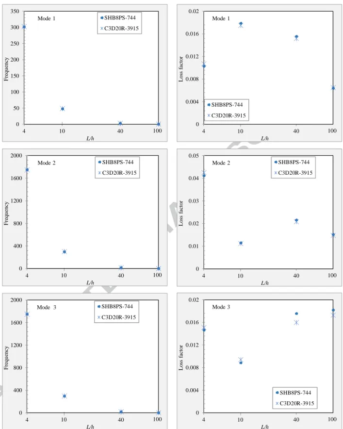
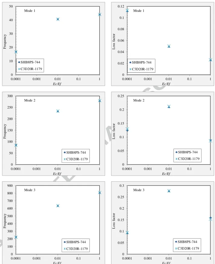
To further validate the proposed approach, an additional investigation is carried out concerning the analysis of damping parameters, which represent the damped frequencies and associated loss factor properties. The SHB8PS solid–shell results are validated through comparisons with the C3D20R quadratic element, the latter having been previously shown to be able to provide reliable reference results. In this last investigation, the same configurations as above, with the same ranges of variation for the various dimensionless beam parameters, are considered again. The results for these three configurations and the associated validations are shown in Figs. 3–5.

Table 11 Influence of hc/hf (L/h = 20, Ec/Ef = 2x10-5_). Elements SHB8PS C3D8 C3D20R NDOF/layer 2160 384000 48000 NIP/element 2 8 8 0.1 c f h h = 21.591 21.638 21.605 122.45 122.43 122.19 337.43 335.46 334.83 1 c f h h = 13.097 13.266 13.102 75.838 77.080 75.970 209.82 212.77 209.63 40 c f h h = 4.2207 4.4651 4.2203 12.285 14.142 12.281 22.082 25.968 22.002 100 c f h h = 4.0513 4.2184 4.0507 12.255 13.086 12.255 21.146 23.361 21.144

Table 12 Influence of L/h (hc/hf = 1, Ec/Ef = 2x10-5). SHB8PS C3D8 C3D20R NDOF/layer 2160 384000 48000 NIP/element 2 8 8 4 L h = 301.43 302.94 301.93 1822.5 1847.2 1822.6 5827.4 5629.1 5834.8 10 L h = 49.087 49.433 49.132 300.42 301.42 300.46 814.33 810.75 815.68 40 L h= 3.9490 4.5161 3.9491 19.987 24.125 19.940 53.314 65.450 53.299 100 L h= 0.9718 1.3365 0.9714 3.9592 6.7934 3.9597 9.4097 18.068 9.4105 Table 13 Influence of Ec/Ef (hc/hf = 1, L/h = 20). SHB8PS C3D8 C3D20R NDOF/layer 2160 384000 48000 NIP/element 2 8 8 4 10 c f E E -= 16.511_80.943 16.767_82.799 16.550_81.068 214.56 219.49 214.44 0.1 c f E E = 42.520 42.640 42.536 252.56 253.18 252.57 657.94 658.87 657.30 100 c f E E = 95.304 97.430 95.860 595.94 607.62 597.92 1666.78 1690.5 1664.5

Fig. 3. Frequencies and loss factors for the first three modes with variation of the thickness ratio hc/hf. 0 5 10 15 20 25 30 0.01 0.1 1 10 100 SHB8PS-378 C3D20R-1179 Mode 1 F re q u en cy hc/hf 0 0.02 0.04 0.06 0.08 0.1 0.12 0.14 0.01 0.1 1 10 100 SHB8PS-378 C3D20R-1179 Mode 1 L o ss fa ct o r hc/hf 0 20 40 60 80 100 120 140 160 0.01 0.1 1 10 100 SHB8PS-378 C3D20R-1179 Mode 2 F re q u en cy hc/hf 0 0.04 0.08 0.12 0.16 0.2 0.01 0.1 1 10 100 SHB8PS-378 C3D20R-1179 Mode 2 L o ss fa ct o r hc/hf 0 50 100 150 200 250 300 350 400 450 0.01 0.1 1 10 100 SHB8PS-378 C3D20R-1179 Mode 3 F re q u en cy hc/hf 0 0.05 0.1 0.15 0.2 0.25 0.3 0.01 0.1 1 10 100 SHB8PS-378 C3D20R-1179 Mode 3 L o ss fa ct o r hc/hf

Fig. 4. Frequencies and loss factors for the first three modes with variation of the length to thickness ratio L/h. 0 50 100 150 200 250 300 350 4 40 SHB8PS-744 C3D20R-3915 Mode 1 F re q u en cy L/h 10 100 0 0.004 0.008 0.012 0.016 0.02 4 40 SHB8PS-744 C3D20R-3915 Mode 1 L o ss fa ct o r L/h 10 100 0 400 800 1200 1600 2000 4 40 SHB8PS-744 C3D20R-3915 Mode 2 F re q u en cy L/h 10 100 0 0.01 0.02 0.03 0.04 0.05 4 40 SHB8PS-744 C3D20R-3915 Mode 2 L o ss fa ct o r L/h 10 100 0 400 800 1200 1600 2000 4 40 SHB8PS-744 C3D20R-3915 Mode 3 F re q u en cy L/h 10 100 0 0.004 0.008 0.012 0.016 0.02 4 40 SHB8PS-744 C3D20R-3915 Mode 3 L o ss fa ct o r L/h 10 100

Fig. 5. Frequencies and loss factors for the first three modes with variation of the layer stiffness ratio Ec/Ef.

0 10 20 30 40 50 0.0001 0.001 0.01 0.1 1 SHB8PS-744 C3D20R-1179 Mode 1 F re q u en cy Ec/Ef 0 0.02 0.04 0.06 0.08 0.1 0.12 0.0001 0.001 0.01 0.1 1 SHB8PS-744 C3D20R-1179 Mode 1 L o ss fa ct o r Ec/Ef 0 50 100 150 200 250 300 0.0001 0.001 0.01 0.1 1 SHB8PS-744 C3D20R-1179 Mode 2 F re q u en cy Ec/Ef 0 0.05 0.1 0.15 0.2 0.25 0.0001 0.001 0.01 0.1 1 SHB8PS-744 C3D20R-1179 Mode 2 L o ss fa ct o r Ec/Ef 0 100 200 300 400 500 600 700 800 900 0.0001 0.001 0.01 0.1 1 SHB8PS-744 C3D20R-1179 Mode 3 F re q u en cy Ec/Ef 0 0.05 0.1 0.15 0.2 0.25 0.3 0.0001 0.001 0.01 0.1 1 SHB8PS-744 C3D20R-1179 Mode 3 L o ss fa ct o r Ec/Ef

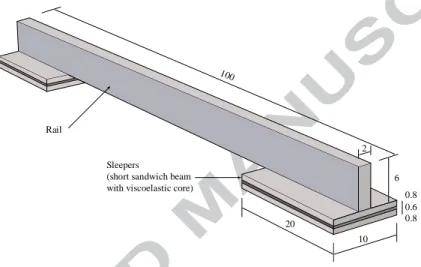
5.3 Application of the proposed model: railway modeling

We consider here a more complex application, which consists of a simplified pattern of rail on sleepers. This analysis is proposed in order to show interest of the proposed model in modeling real structures. As shown in Fig. 6, the structure consists of a section of a rail on two sleepers, which may be modeled by short beams with viscoelastic sandwich core, fixed on an assumed rigid ground. We are interested here in buckling modes that can cause the derailment of a train. This system may also help to damp vibrations caused by trains. The rail and the elastic faces of the short beams are made of steel, whose material properties are given in Table 14. The viscoelastic core is made of ISD112, whose parameters were previously reported in Tables 9 and 10. The geometric parameters of the studied structure are listed in Fig. 6.

Fig. 6. Rail on sleepers modeled by short sandwich beams with viscoelastic core.

Table 14 Steel properties.

steel

E n_steel r_steel

2.1x1011_{Pa 0.3 7800 kg.m}-3

The analysis of the structure consisted in an evaluation of the damping properties, which are the frequencies and loss factors. The first three modes of this model of rail on sleepers are shown in Fig. 7. The simulation results given by the proposed solid–shell modeling approach are compared to the results yielded by the C3D20R element, which served as reference (see Table 15). The obtained results are rather satisfactory since they are in agreement with those given by the C3D20R Abaqus element. It is noteworthy, however, that the proposed solid–shell modeling approach requires much fewer degrees of freedom to achieve convergence with sufficient accuracy, which confirms its efficiency and its interest in terms of computational effort reduction.

100 6 0.8 0.8 0.6 10 20 2 Sleepers

(short sandwich beam with viscoelastic core) Rail

Fig. 7. First three modes for the model of rail on sleepers.

Table 15

Frequencies and loss factors associated with the first three modes of the rail on sleepers.

SHB8PS C3D20R NDOF ₁₉₂₆ 9168 NIP/element 2 8 Eigen frequency Damped

frequency Loss factor

Eigen frequency

Damped

frequency Loss factor

1 163.17 165.23 6.22e-2 163.07 165.31 5.51e-2

2 361.62 370.80 1.08e-1 357.28 366.83 1.03e-1

3 620.16 637.13 9.62e-2 604.54 617.78 9.83e-2

6. Conclusions

In this contribution, a new modeling approach of frequency dependent viscoelastic sandwich structures has been proposed for vibration analysis. To this end, the free vibration problem was solved by coupling a solid–shell finite element and the Diamant approach. Different material and geometric configurations were investigated, which include parameter values ranging beyond the classical model limitations pointed out in [17]. The obtained results emphasize the advantages of adopting the proposed solid– shell concept in this type of applications and the associated benefits, especially in terms of coarse-mesh accuracy and efficient kinematic description. This study will be extended to nonlinear vibrations of sandwich structures including plates. Another possible extension would be the modeling of multilayer structures using a single layer of elements with the possibility of assigning various material responses at different integration points.

References

[1] Kerwin EM. Damping of flexural waves by a constrained viscoelastic layer. J Acoust Soc Am 1959;31:952–962.

[2] Ross D, Ungar E, Kerwin EM. Damping of plate flexural vibrations by means of viscoelastic laminae. In: Ruzicka JE, editor, Structural damping, 1959.

[3] Rao DK. Frequency and loss factors of sandwich beams under various boundary conditions. J Mech Engng Sci 1978;20:271–282.

[4] Reissner E. The effect of transverse shear deformation on the bending of elastic plates. J Appl Mech 1945;12:69–75.

[5] Mindlin RD. Influence of rotatory inertia and shear in flexural motions of isotropic elastic plates. J Appl Mech 1951;18:1031–1036.

[6] Reddy JN. A simple higher-order theory for laminated composite plates. J Appl Mech 1984;51:745–752.

[7] Touratier M. An efficient standard plate theory. Int J Eng Sci 1991;29:901–916. [8] Lu YP, Killian JW, Everstine GC. Vibrations of three layered damped sandwich

plate composites. J Sound Vibr 1979;64:63–71.

[9] Johnson CD, Kienholz DA, Rogers LC. Finite element prediction of damping in beams with constrained viscoelastic layer. Shock Vibr Bull 1981;51:71–81.

[10] Ramesh TC, Ganesan N. Finite element analysis of conical shells with a constrained viscoelastic layer. J Sound Vibr 1994:171:577–601.

[11] Sainsbury MG, Zhang QJ. The Galerkin element method applied to the vibration of damped sandwich beams. Comput Struct 1999;71:239–256.

[12] Carrera E. Historical review of Zig-Zag theories for multilayered plates and shells. App Mech Rev 2003;56:287–308.

[13] Carrera E. Theories and finite elements for multilayered, anisotropic, composite plates and shells. Arch Comput Meth Eng 2002;9:87–140.

[14] Boudaoud H, Daya EM, Belouettar S, Duigou L, Potier-Ferry M. Damping analysis of beams submitted to passive and active control. Eng Struct 2009;31:322–331.

[15] Bilasse M, Daya EM, Azrar L. Linear and nonlinear vibrations analysis of viscoelastic sandwich beams. J Sound Vib 2010;329:4950–4969.

[16] Abdoun F, Azrar L, Daya EM, Potier-Ferry M. Forced harmonic response of viscoelastic structures by an asymptotic numerical method. Comput Struct 2009;87:91–100.

[17] Hu H, Belouettar S, Potier-Ferry M, Daya EM. Review and assessment of various theories for modeling sandwich composites. Compos Struct 2008;84:282–292.

[18] Carrera E. Theories and finite elements for multilayered plates and shells: a unified compact formulation with numerical assessment and benchmarking. Arch Comput Meth Eng 2003;10:216–296.

[19] Abed-Meraim F, Combescure A. SHB8PS – a new adaptive assumed-strain continuum mechanics shell element for impact analysis. Comput Struct 2002;80:791–803.

[20] Abed-Meraim F, Combescure A. An improved assumed-strain solid–shell element formulation with physical stabilization for geometric nonlinear applications and elastic–plastic stability analysis. Int J Numer Meth Eng 2009;80:1640–1686. [21] Legay A, Combescure A. Elastoplastic stability analysis of shells using the

physically stabilized finite element SHB8PS. Int J Numer Meth Eng 2003;57:1299–1322.

[22] Belytschko T, Bindeman LP. Assumed strain stabilization of the eight node hexahedral element. Comput Meth App Mech Eng 1993;105:225–260.

[23] Salahouelhadj A, Abed-Meraim F, Chalal H, Balan T. Application of the continuum shell finite element SHB8PS to sheet forming simulation using an extended large strain anisotropic elastic–plastic formulation. Arch Appl Mech 2012;82:1269–1290.

[24] Wilkinson JH. The Algebraic Eigenvalue Problem. Clarendon Press, Oxford, 1965.

[25] Bathe KJ. Finite Element Procedures in Engineering Analysis. Prentice-Hall, NJ, 1982.

[26] Ungar EE, Kerwin EM. Loss factors of viscoelastic systems in terms of energy concepts. J Acoust Soc Am 1962;34:954–957.

[27] Rikards R, Chate A, Barkanov E. Finite element analysis of damping the vibrations of laminated composites. Comput Struct 1993;47:1005–1015.

[28] Soni ML. Finite element analysis of viscoelastically damped sandwich structures. Shock Vibr Bull 1981;55:97–109.

[29] Ma BA, He JF. A finite element analysis of viscoelastically damped sandwich plates. J Sound Vibr 1992;152:107–123.

[30] Chen X, Chen HL, Hu XL. Damping prediction of sandwich structures by order-reduction-iteration approach. J Sound Vibr 1999;222:803–812.

[31] Daya EM, Potier-Ferry M. A numerical method for nonlinear eigenvalue problems application to vibrations of viscoelastic structures. Comput Struct 2001;79:533–541.

[32] Duigou L, Daya EM, Potier-Ferry M. Iterative algorithms for non-linear eigenvalue problems. Application to vibrations of viscoelastic shells. Comput Meth App Mech Eng 2003;192:1323–1335.

[33] Damil N, Potier-Ferry M, Najah A, Chari R, Lahmam H. An iterative method based upon padé approximants. Commun Numer Meth Eng 1999;15:701–708.

[34] Thompson JMT, Walker AC. The non-linear perturbation analysis of discrete structure systems. Int J Solid Struct 1968;4:219–259.

[35] Boumediene F, Cadou JM, Duigou L, Daya EM. A reduction model for eigensolutions of damped viscoelastic sandwich structures. Mechanics Research Communications 2014;57:74–81.

[36] Flanagan DP, Belytschko T. A uniform strain hexahedron and quadrilateral with orthogonal hourglass control. Int J Numer Meth Eng 198;17:679–706.

[37] Charpentier I, Potier-Ferry M. Différentiation automatique de la méthode asymptotique numérique typée : l’approche Diamant. Comptes Rendus Mécanique 2008;336:336–340.

[38] Koutsawa Y, Charpentier I, Daya EM, Cherkaoui M. A generic approach for the solution of nonlinear residual equations. Part I: The Diamant toolbox. Comput Meth Appl Mech Eng 2008;198:572–577.

[39] Bilasse M, Charpentier I, Daya EM, Koutsawa Y. A generic approach for the solution of nonlinear residual equations. Part II: Homotopy and complex nonlinear eigenvalue method. Comput Meth Appl Mech Eng 2009;198:3999– 4004.

[40] Lampoh M, Charpentier I, Daya EM. A generic approach for the solution of nonlinear residual equations. Part III: Sensitivity computations. Comput Meth Appl Mech Eng 2011;200:2983–2990.