HAL Id: hal-00412946
https://hal.archives-ouvertes.fr/hal-00412946
Submitted on 15 Apr 2020
HAL is a multi-disciplinary open access
archive for the deposit and dissemination of
sci-entific research documents, whether they are
pub-lished or not. The documents may come from
teaching and research institutions in France or
abroad, or from public or private research centers.
L’archive ouverte pluridisciplinaire HAL, est
destinée au dépôt et à la diffusion de documents
scientifiques de niveau recherche, publiés ou non,
émanant des établissements d’enseignement et de
recherche français ou étrangers, des laboratoires
publics ou privés.
Causal graphical models with latent variables: Learning
and inference
Stijn Meganck, Philippe Leray, Bernard Manderick
To cite this version:
Stijn Meganck, Philippe Leray, Bernard Manderick. Causal graphical models with latent variables:
Learning and inference. ECSQARU, 2007, Hammamet, Tunisia. pp.5-16,
�10.1007/978-3-540-75256-1_4�. �hal-00412946�
Causal Graphical Models with Latent Variables:
Learning and Inference
Stijn Meganck1, Philippe Leray2, and Bernard Manderick1
1 CoMo, Vrije Universiteit Brussel, 1050 Brussels, Belgium,
WWW home page: http://como.vub.ac.be/Members/stijn/stijn.html
2 LITIS EA 4051, INSA Rouen, St. Etienne du Rouvray, France,
Abstract. Several paradigms exist for modeling causal graphical models
for discrete variables that can handle latent variables without explicitly modeling them quantitatively. Applying them to a problem domain con-sists of different steps: structure learning, parameter learning and using them for probabilistic or causal inference. We discuss two well-known formalisms, namely semi-Markovian causal models and maximal ances-tral graphs and indicate their strengths and limitations. Previously an algorithm has been constructed that by combining elements from both techniques allows to learn a semi-Markovian causal models from a mix-ture of observational and experimental data. The goal of this paper is to recapitulate the integral learning process from observational and experi-mental data and to demonstrate how different types of inference can be performed efficiently in the learned models. We will do this by proposing an alternative representation for semi-Markovian causal models.
1
Introduction
This paper discusses causal graphical models for discrete variables that can han-dle latent variables without explicitly modeling them quantitatively. In the un-certainty in artificial intelligence area there exist several paradigms for such problem domains. Two of them are semi-Markovian causal models and maxi-mal ancestral graphs. Applying these techniques to a problem domain consists of several steps, typically: structure learning from observational and experimen-tal data, parameter learning, probabilistic inference, and, quantitative causal inference.
Semi-Markovian causal models (SMCMs) are an approach developed by Tian and Pearl [1, 2]. They are specifically suited for performing quantitative causal inference in the presence of latent variables. However, at this time no efficient parametrisation of such models is provided and there is no algorithm for per-forming efficient probabilistic inference. Furthermore there are no techniques to learn these models from data issued from observations, experiments or both.
Maximal ancestral graphs (MAGs) [3] are specifically suited for structure learning in the presence of latent variables from observational data. However, the techniques only learn up to Markov equivalence and provide no clues on
which additional experiments to perform in order to obtain the fully oriented causal graph. See [4, 5] for that type of results for Bayesian networks without latent variables. Furthermore, as of yet no parametrisation for discrete variables is provided for MAGs and no techniques for probabilistic inference have been developed. There is some work on algorithms for causal inference, but it is re-stricted to causal inference quantities that are the same for an entire Markov equivalence class of MAGs [6, 7].
We have chosen to use SMCMs as a final representation in our work, because they are the only formalism that allows to perform causal inference while fully taking into account the influence of latent variables. However, we will combine existing techniques to learn MAGs with newly developed methods to provide an integral approach that uses both observational data and experiments in order to learn fully oriented semi-Markovian causal models.
Furthermore, we have developed an alternative representation for the proba-bility distribution represented by a SMCM, together with a parametrisation for this representation, where the parameters can be learned from data with clas-sical techniques. Finally, we discuss how probabilistic and quantitative causal inference can be performed in these models with the help of the alternative representation and its associated parametrisation.
The next section introduces some notations and definitions and we discuss causal models with latent variables. After that we discuss structure learning for those models and in the next section we introduce techniques for learning a SMCM with the help of experiments. Then we introduce a new representation for SMCMs that can easily be parametrised. We also show how both probabilistic and causal inference can be performed with the help of this new representation.
2
Preliminaries
We start this section by introducing basic notations necessary for the under-standing of the rest of this paper. Then we will discuss classical probabilistic Bayesian networks followed by causal Bayesian networks. Finally we handle the difference between probabilistic and causal inference, or observation vs. manip-ulation.
2.1 Notations
In this work uppercase letters are used to represent variables or sets of variables, i.e. V = {V1, . . . , Vn}, while corresponding lowercase letters are used to represent their instantiations, i.e. v1, v2and v is an instantiation of all vi. P (Vi) is used to denote the probability distribution over all possible values of variable Vi, while P(Vi = vi) is used to denote the probability of the instantiation of variable Vi to value vi. Usually, P (vi) is used as an abbreviation of P (Vi= vi).
The operators P a(Vi), Anc(Vi), N e(Vi) denote the observable parents, ances-tors and neighbors respectively of variable Vi in a graph and P a(vi) represents
the values of the parents of Vi. If Vi ↔ Vj appears in a graph then we say that they are spouses, i.e. Vi ∈ Sp(Vj) and vice versa.
When two variables Vi, Vj are independent we denote it by (Vi⊥⊥Vj), when they are dependent by (Vi 2Vj).
2.2 Definitions
Both techniques are an extension of causal Bayesian networks for modeling sys-tems without latent variables.
Definition 1. A causal Bayesian network is a triple hV, G, P (vi|P a(vi))i, with:
– V = {V1, . . . , Vn}, a set of observable discrete random variables
– a directed acyclic graph (DAG) G, where each node represents a variable from V
– parameters: conditional probability distributions (CPD) P (vi|P a(vi)) of each variable Vi from V conditional on its parents in the graph G.
– Furthermore, the directed edges in G represent autonomous causal relations between the corresponding variables.
The interpretation of directed edges is different from a classical BN, where the arrows only represent a probabilistic dependency, and not necessarily a causal one.
This means that in a CBN, each CPD P (vi|P a(vi)) represents a stochastic assignment process by which the values of Viare chosen in response to the values of P a(Vi) in the underlying domain. This is an approximation of how events are physically related with their effects in the domain that is being modeled. For such an assignment process to be autonomous means that it must stay invariant under variations in the processes governing other variables [1].
In the above we made the assumption of causal sufficiency, i.e. that for every variable of the domain that is a common cause, observational data can be obtained in order to learn the structure of the graph and the CPDs. Often this assumption is not realistic, as it is not uncommon that a subset of all the variables in the domain is never observed. We refer to such a variable as a latent variable.
The central graphical modeling representation that we use are the semi-Markovian causal models. They were first used by Pearl [1], and Pearl and Tian [2] have developed causal inference algorithms for them.
Definition 2. A semi-Markovian causal model (SMCM) is an acyclic causal graph G with both directed and bi-directed edges. The nodes in the graph repre-sent observable variables V = {V1, . . . , Vn} and the bi-directed edges implicitly represent latent variables L = {L1, . . . , Ln′}.
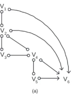
See Figure 1(b) for an example SMCM representing the underlying DAG in (a).
V3 V1 V2 V5 V4 V6 L 1 L2 V3 V1 V2 V5 V4 V6 (a) (b) V3 V1 V2 V5 V4 V6 (c)
Fig. 1. (a) A problem domain represented by a causal DAG model with observable
and latent variables. (b) A semi-Markovian causal model representation of (a). (c) A maximal ancestral graph representation of (a).
Maximal ancestral graphs are another approach to modeling with latent vari-ables [3]. The main research focus in that area lies on learning the structure of these models and on representing exactly all the independences between the observable variables of the underlying DAG.
Ancestral graphs (AGs) are graphs that are complete under marginalisation and conditioning. We will only discuss AGs without conditioning as is commonly done in recent work [8–10].
Definition 3. An ancestral graph without conditioning is a graph with no directed cycle containing directed → and bi-directed ↔ edges, such that there is no bi-directed edge between two variables that are connected by a directed path.
Definition 4. An ancestral graph is said to be a maximal ancestral graph if, for every pair of non-adjacent nodes Vi, Vj there exists a set Z such that Vi and Vj are d-separated given Z.
See Figure 1(c) for an example MAG representing the underlying DAG in (a) and corresponding to the SMCM in (b).
Definition 5. Let [G] be the Markov equivalence class for an arbitrary MAG G. The complete partial ancestral graph (CPAG) for [G], PG, is a graph with possibly the following edges →, ↔, o−o, o→, such that
1. PG has the same adjacencies as G (and hence any member of [G]) does; 2. A mark of arrowhead (>) is in PG if and only if it is invariant in [G]; and 3. A mark of tail (−) is in PG if and only if it is invariant in [G].
4. A mark of (o) is in PG if not all members in [G] have the same mark.
V3 V1 V2 V5 V4 V6 (a)
Fig. 2.The CPAG corresponding to the MAG in Figure 1(c).
3
Structure Learning with Latent Variables
Just as learning a graphical model in general, learning a model with latent vari-ables consists of two parts: structure learning and parameter learning. Both can be done using data, expert knowledge and/or experiments. In this section we dis-cuss structure learning and we differentiate between learning from observational and experimental data.
3.1 Learning from observational data
In the literature no algorithm for learning the structure of an SMCM exists. In order to learn MAGs from observational data a constraint based learning algo-rithm has been developed. It is called the Fast Causal Inference (FCI) algoalgo-rithm [11] and it uses conditional independence relations found between observable variables to learn a structure. Recently this result has been extended with the complete tail augmentation rules introduced in [12]. The results of this algo-rithm is a complete partial ancestral graph (CPAG), representing the Markov equivalence class of MAGs consistent with the data.
In a CPAG the directed edges have to be interpreted as representing ancestral relations instead of immediate causal relations. More precisely, this means that there is a directed edge from Vito Vj if Viis an ancestor of Vj in the underlying DAG and there is no subset of observable variables D such that (Vi⊥⊥Vj|D). This does not necessarily mean that Vihas an immediate causal influence on Vj, it may also be a result of an inducing path between Viand Vj. An inducing path between Vi and Vj is a path that can not be blocked by any subset of variables, the official definition is given below:
Definition 6. An inducing path is a path in a graph such that each observable non-endpoint node is a collider, and an ancestor of at least one of the endpoints. A consequence of these properties of MAGs and CPAGs is that they are not very suited for general causal inference, since the immediate causal parents of each observable variable are not available and this information is needed to
perform the calculations. As we want to learn models that can perform causal inference, we will discuss how to transform a CPAG into a SMCM next and hence introduce a learning algorithm for SMCMs using both observational and experimental data.
3.2 Learning from experimental data
As mentioned above, the result of current state-of-the-art techniques that learn models with implicit latent variables from observational data is a CPAG. This is a representative of the Markov equivalence class of MAGs. Any MAG in that class will be able to represent the same JPD over the observable variables, but not all those MAGs will have all edges with a correct causal orientation.
Furthermore in MAGs the directed edges do not necessarily have an imme-diate causal meaning as in CBNs or SMCMs, instead they have an ancestral meaning. If it is your goal to perform causal inference, you will need to know the immediate parents to be able to reason about all causal queries.
MAGs are maximal, thus every missing edge must represent a conditional independence. In the case that there is an inducing path between two variables and no edge in the underlying DAG, the result of the current learning algorithms will be to add an edge between the variables. Again, although these type of edges give the only correct representation of the conditional independence relations in the domain, they do not represent an immediate causal relation (if the inducing edge is directed) or a real latent common cause (if the inducing edge is bi-directed). Because of this they could interfere with causal inference algorithms, therefore we would like to identify and remove these type of edges.
To recapitulate, the goal of techniques aiming at transforming a CPAG must be twofold:
– finding the correct causal orientation of edges that are not completely spec-ified by the CPAG (o→ or o−o), and,
– removing edges due to inducing paths.
For the details of the learning algorithm we refer to [13] and [14]. For the re-mainder of the paper we will focus on constructing an alternative representation for SMCMs in order to perform inference.
4
Parametrisation of SMCMs
In his work on causal inference, Tian provides an algorithm for performing causal inference given knowledge of the structure of an SMCM and the joint probability distribution (JPD) over the observable variables. However, a parametrisation to efficiently store the JPD over the observables is not provided.
We start this section by discussing the factorisation for SMCMs introduced in [2]. From that result we derive an additional representation for SMCMs and a parametrisation of that representation that facilitates probabilistic and causal inference. We will also discuss how these parameters can be learned from data.
4.1 Factorising with Latent Variables
Consider an underlying DAG with observable variables V = {V1, . . . , Vn} and latent variables L = {L1, . . . , Ln′}. Then the joint probability distribution can
be written as the following mixture of products:
P(v) = X {lk|Lk∈L}
Y Vi∈V
P(vi|P a(vi), LP a(vi))Y Lj∈L
P(lj), (1)
where LP a(vi) are the latent parents of variable Vi.
Remember that in a SMCM the latent variables are implicitly represented by bi-directed edges, then consider the following definition.
Definition 7. In a SMCM, the set of observable variables can be partitioned into disjoint groups by assigning two variables to the same group iff they are connected by a bi-directed path. We call such a group a c-component (from ”confounded component”) [2].
E.g. in Figure 1(b) variables V2, V5, V6 belong to the same c-component. Then it can be readily seen that c-components and their associated latent variables form respective partitions of the observable and latent variables. Let Q[Si] denote the contribution of a c-component with observable variables Si ⊂ V to the mixture of products in equation 1. Then we can rewrite the JPD as follows: P(v) = Q
i∈{1,...,k} Q[Si].
Finally, in [2] it is shown that each Q[S] could be calculated as follows. Let Vo1 < . . . < Von be a topological order over V , and let V
(i) = {Vo 1, . . . , Voi}, i= 1, . . . , n and V(0)= ∅. Q[S] = Y Vi∈S P(vi|(Ti∪ P a(Ti))\{Vi}) (2)
where Ti is the c-component of the SMCM G reduced to variables V(i), that contains Vi. The SMCM G reduced to a set of variables V′ ⊂ V is the graph obtained by removing all variables V \V′ from the graph and the edges that are connected to them.
In the rest of this section we will develop a method for deriving a DAG from a SMCM. We will show that the classical factorisationQP(vi|P a(vi)) associated with this DAG, is the same as the one that is associated with the SMCM as above.
4.2 Parametrised representation
Here we first introduce an additional representation for SMCMs, then we show how it can be parametrised and finally, we discuss how this new representation could be optimised.
Given a SMCM G and a topological order O, the PR-representation has these properties: 1. The nodes are V , the observable variables of the SMCM. 2. The directed edges that are present in the SMCM are also
present in the PR-representation.
3. The bi-directed edges in the SMCM are replaced by a number of directed edges in the following way:
Add an edge from node Vi to node Vj iff:
a) Vi∈(Tj∪ P a(Tj)), where Tj is the c-component of G
reduced to variables V(j)that contains Vj,
b) except if there was already an edge between nodes Viand Vj.
Table 1.Obtaining the parametrised representation from a SMCM.
V3 V1 V2 V5 V4 V6 V1,V2,V4,V5,V6 V2,V3,V4 V2,V4 (a) (b)
Fig. 3.(a) The PR-representation applied to the SMCM of Figure 1(b). (b) Junction
tree representation of the DAG in (a).
PR-representation Consider Vo1 < . . . < Von to be a topological order O over the observable variables V , and let V(i)= {Vo
1, . . . , Voi}, i = 1, . . . , n and
V(0) = ∅. Then Table 1 shows how the parametrised (PR-) representation can be obtained from the original SMCM structure.
What happens is that each variable becomes a child of the variables it would condition on in the calculation of the contribution of its c-component as in Equation (2).
In Figure 3(a), the PR-representation of the SMCM in Figure 1(a) can be seen. The topological order that was used here is V1< V2< V3< V4< V5< V6 and the directed edges that have been added are V1→ V5, V2 → V5, V1→ V6, V2→ V6, and, V5→ V6.
The resulting DAG is an I -map [15], over the observable variables of the independence model represented by the SMCM. This means that all the inde-pendences that can be derived from the new graph must also be present in the JPD over the observable variables. This property can be more formally stated as the following theorem.
Theorem 1. The PR-representation P R derived from a SMCM S is an I-map of that SMCM.
Proof. Proving that P R is an I -map of S amounts to proving that all indepen-dences represented in P R (A) imply an independence in S (B), or A ⇒ B. We will prove that assuming both A and ¬B leads to a contradiction.
Assumption ¬B: consider that two observable variables X and Y are depen-dent in the SMCM S conditional on some (possible empty) set of observable variables Z: X 2SY|Z.
Assumption A: consider that X and Y are independent in P R conditional on Z: X⊥⊥P RY|Z.
Then based on X 2SY|Z we can discriminate two general cases:
1. ∃ a path C in S connecting variables X and Y that contains no colliders and no elements of Z.
2. ∃ a path C in S connecting variables X and Y that contains at least one collider Zi that is an element of Z. For the collider there are three possibil-ities:
(a) X . . . Ci→ Zi← Cj. . . Y (b) X . . . Ci↔ Zi← Cj. . . Y (c) X . . . Ci↔ Zi↔ Cj. . . Y
Now we will show that each case implies ¬A:
1. Transforming S into P R only adds edges and transforms double-headed edges into single headed edges, hence the path C is still present in S and it still contains no collider. This implies that X⊥⊥P RY|Z is false.
2. (a) The path C is still present in S together with the collider in Zi, as it has single headed incoming edges. This implies that X⊥⊥P RY|Z is false. (b) The path C is still present in S. However, the double-headed edge is
transformed into a single headed edge. Depending on the topological order there are two possibilities:
– Ci → Zi ← Cj: in this case the collider is still present in P R, this implies that X 2P RY|Z
– Ci ← Zi← Cj: in this case the collider is no longer present, but in P Rthere is the new edge Ci← Cj and hence X 2P RY|Z
(c) The path C is still present in S. However, both double-headed edges are transformed into single headed edges. Depending on the topological order there are several possibilities. For the sake of brevity we will only treat a single order here, for the others it can easily be checked that the same holds.
If the order is Ci< Zi < Cj, the graph becomes Ci→ Zi→ Cj, but there are also edges from Ci and Zi to Cj and its parents P a(Cj). Thus the collider is no longer present, but the extra edges ensure that X 2P RY|Z.
This implies that X⊥⊥P RY|Z is false and therefore we can conclude that P R is always an I -map of S under our assumptions. ⊓⊔
Parametrisation For this DAG we can use the same parametrisation as for classical BNs, i.e. learning P (vi|P a(vi)) for each variable, where P a(vi) denotes the parents in the new DAG. In this way the JPD over the observable vari-ables factorises as in a classical BN, i.e. P (v) = QP(vi|P a(vi)). This follows immediately from the definition of a c-component and from Equation (2).
Optimising the Parametrisation Remark that the number of edges added during the creation of the PR-representation depends on the topological order of the SMCM.
As this order is not unique, giving precedence to variables with a lesser amount of parents, will cause less edges to be added to the DAG. This is because added edges go from parents of c-component members to c-component members that are topological descendants.
By choosing an optimal topological order, we can conserve more conditional independence relations of the SMCM and thus make the graph more sparse, leading to a more efficient parametrisation.
Note that the choice of the topological order does not influence the correct-ness of the representation, Theorem 1 shows that it will always be an I -map.
4.3 Probabilistic inference
Two of the most famous existing probabilistic inference algorithms for models without latent variables are the λ − π algorithm [15] for tree-structured BNs, and the junction tree algorithm [16] for arbitrary BNs.
These techniques cannot immediately be applied to SMCMs for two reasons. First of all until now no efficient parametrisation for this type of models was available, and secondly, it is not clear how to handle the bi-directed edges that are present in SMCMs.
We have solved this problem by first transforming the SMCM to its PR-representation which allows us to apply the junction tree (JT) inference al-gorithm. This is a consequence of the fact that, as previously mentioned, the PR-representation is an I -map over the observable variables. And as the JT algorithm only uses independences in the DAG, applying it to an I -map of the problem gives correct results. See Figure 3(b) for the junction tree obtained from the parametrised representation in Figure 3(a). Although this seems to be a minor improvement in this example, it has to be noted that this is the best possible results for this structure. The complexity of the junction tree in general will be dependent on the structure between the observed variables and on the complexity of the c-components.
4.4 Causal inference
In [2], an algorithm for performing causal inference was developed, however as mentioned before they have not provided an efficient parametrisation.
In [6, 7], a procedure is discussed that can identify a limited amount of causal inference queries. More precisely only those whose result is equal for all the members of a Markov equivalence class represented by a CPAG.
In [17], causal inference in AGs is shown on an example, but a detailed approach is not provided and the problem of what to do when some of the parents of a variable are latent is not solved.
By definition in the PR-representation, the parents of each variable are ex-actly those variables that have to be conditioned on in order to obtain the factor of that variable in the calculation of the c-component, see Table 1 and [2]. Thus, the PR-representation provides all the necessary quantitative information, while the original structure of the SMCM provides the necessary structural informa-tion, for Tian’s algorithm to be applied.
5
Conclusions and Perspectives
In this paper we have introduced techniques for causal graphical modeling with latent variables. We pointed out that none of the existing techniques provide a complete answer to the problem of modeling systems with latent variables.
We have discussed concisely the structure learning process and in more de-tail the parametrisation of the model and probabilistic and causal inference. As the experimental structure learning approach relies on randomized controlled experiments, in general it is not scalable to problems with a large number of variables, due to the associated large number of experiments. Furthermore, it cannot be applied in application areas where such experiments are not feasible due to practical or ethical reasons.
SMCMs have not been parametrised in another way than by the entire joint probability distribution, we showed that using an alternative representation, we can parametrise SMCMs in order to perform probabilistic as well as causal inference. Furthermore this new representation allows to learn the parameters using classical methods.
We have informally pointed out that the choice of a topological order when creating the PR-representation, influences the size and thus the efficiency of the PR-representation. We would like to investigate this property in a more formal manner. Finally, we have started implementing the techniques introduced in this paper into the structure learning package (SLP)3 of the Bayesian networks toolbox (BNT)4 for MATLAB.
Acknowledgements
This work was partially supported by the IST Programme of the European Community, under the PASCAL network of Excellence, IST-2002-506778. This publication only reflects the authors’ views.
3 http://banquiseasi.insa-rouen.fr/projects/bnt-slp/
References
1. Pearl, J.: Causality: Models, Reasoning and Inference. MIT Press (2000)
2. Tian, J., Pearl, J.: On the identification of causal effects. Technical Report (R-290-L), UCLA C.S. Lab (2002)
3. Richardson, T., Spirtes, P.: Ancestral graph markov models. Technical Report 375, Dept. of Statistics, University of Washington (2002)
4. Eberhardt, F., Glymour, C., Scheines, R.: On the number of experiments sufficient and in the worst case necessary to identify all causal relations among n variables. In: Proc. of the 21st Conference on Uncertainty in Artificial Intelligence (UAI). (2005) 178–183
5. Meganck, S., Leray, P., Manderick, B.: Learning causal bayesian networks from ob-servations and experiments: A decision theoretic approach. In: Modeling Decisions in Artificial Intelligence, LNCS. (2006) 58–69
6. Spirtes, P., Glymour, C., Scheines, R.: Causation, Prediction and Search. MIT Press (2000)
7. Zhang, J.: Causal Inference and Reasoning in Causally Insufficient Systems. PhD thesis, Carnegie Mellon University (2006)
8. Zhang, J., Spirtes, P.: A transformational characterization of markov equivalence for directed acyclic graphs with latent variables. In: Proc. of the 21st Conference on Uncertainty in Artificial Intelligence (UAI). (2005) 667–674
9. Tian, J.: Generating markov equivalent maximal ancestral graphs by single edge replacement. In: Proc. of the 21st Conference on Uncertainty in Artificial Intelli-gence (UAI). (2005) 591–598
10. Ali, A.R., Richardson, T., Spirtes, P., Zhang, J.: Orientation rules for constructing markov equivalence classes of maximal ancestral graphs. Technical Report 476, Dept. of Statistics, University of Washington (2005)
11. Spirtes, P., Meek, C., Richardson, T.: An algorithm for causal inference in the presence of latent variables and selection bias. In: Computation, Causation, and Discovery. AAAI Press, Menlo Park, CA (1999) 211–252
12. Zhang, J., Spirtes, P.: A characterization of markov equivalence classes for ancestral graphical models. Technical Report 168, Dept. of Philosophy, Carnegie-Mellon University (2005)
13. Maes, S., Meganck, S., Leray, P.: An integral approach to causal inference with la-tent variables. In: Causality and Probability in the Sciences (Texts in Philosophy), (College Publications)
14. Meganck, S., Maes, S., Leray, P., Manderick, B.: Learning semi-markovian causal models using experiments. In: Proceedings of The third European Workshop on Probabilistic Graphical Models , PGM 06. (2006)
15. Pearl, J.: Probabilistic Reasoning in Intelligent Systems. Morgan Kaufmann (1988)
16. Lauritzen, S.L., Spiegelhalter, D.J.: Local computations with probabilities on
graphical structures and their application to expert systems. Journal of the Royal Statistical Society, series B 50 (1988) 157–244
17. Richardson, T., Spirtes, P.: Causal inference via ancestral graph models. In: Oxford Statistical Science Series: Highly Structured Stochastic Systems, Oxford University Press (2003)