Interval Type-2 Fuzzy Gain-adaptive Controller Of A Doubly Fed Induction Machine (dfim)

Journal of Fundamental and Applied Sciences is licensed under a Creative Commons Attribution-NonCommercial 4.0 International License. Libraries Resource Directory. We are listed under Research Associations category.

INTERVAL TYPE-2 FUZZY GAIN-ADAPTIVE CONTROLLER OF A DOUBLY FED INDUCTION MACHINE (DFIM)

K. Loukal* and L. Benalia

LGE Research Laboratory, Department of Electrical Engineering, Faculty of Technology, University Mohamed Boudiaf of M’sila

BP 166 Ichbilia 28000 Algeria

Received: 02 February 2016 / Accepted: 28 April 2016 / Published online: 01 May 2016

ABSTRACT

This paper presents a comparison between an Interval Type-2 Fuzzy Gain-Adaptive IP (IT2FGAIP) controller and a conventional IP controller used for speed control with a direct stator flux orientation control of a doubly fed induction motor. In particular, the introduction part of the paper presents a Direct Stator Flux Orientation Control (DSFOC), the first part of this paper presents a description of the mathematical model of DFIM, and an adaptive IP controller is proposed for the speed control of DFIM in the presence of the variations parametric, A interval type-2 fuzzy inference system is used to adjust in real-time the controller gains. The obtained results show the efficacy of the proposed method.

Keywords: doubly fed induction motor; DFIM; direct stator flux orientation control; interval type-2 fuzzy gain-adaptive IP controller; IT2FGAIP; IP controller.

Author Correspondence, e-mail: muohtlek@yahoo.fr

doi: http://dx.doi.org/10.4314/jfas.v8i2.20

ISSN 1112-9867

1. INTRODUCTION

In recent years, the use of doubly fed induction machine (DFIM) is a best solution for applications where the torque is proportional to the square of the speed; DFIM is an asynchronous wound-rotor machine whose stator and rotor windings are connected to electrical sources. [1-2]

The advantages of DFIM in motor operation for high power applications such as traction, marine propulsion or as a generator in wind systems [3-5], the many benefits of this machine are: reduced manufacturing cost, relatively simple construction, higher speed and do not require ongoing maintenance. For operation at different speeds must be inserted in the machine a converter PWM (Pulse Width Modulation) between the machine and the network. For, whatever the speed of the machine, the voltage is rectified and an inverter connected to the network side is responsible for ensuring consistency between the network frequency and that delivered by the device. The DFIM is essentially nonlinear, due to the coupling between the flux and the electromagnetic torque. The vector control or field orientation control that allows a decoupling between the torque and the flux. [6-8]

With the field orientation control (FOC) method, induction machine drives are becoming a major candidate in high-performance motion control applications, where servo quality operation is required. Fast transient response is made possible by decoupled torque and flux control. The most widely used control method is perhaps the proportional integral control (PI). It is easy to design and implement, but it has difficulty in dealing with parameter variations, and load disturbances [9]. Recent literature has paid much attention to the potential of Gain Adaptive control in machine drive applications.

A number of methods have been proposed in the literature for nonlinear Adaptive applied to the DFIM. A Speed Sensorless Sliding-Mode Controller for DFIM Drives with Adaptive Backstepping Observer in [10] and Robust Speed Sensorless Control Based on Input-output Feedback Linearization Control Using a Sliding-mode Observer in [11].

Our purpose in this paper is to introduce an IT2FGAIP control for DFIM drive system; Fuzzy logic, whose theoretical bases have been established since the early 1960, allows exploiting the linguistic information describing the dynamic behavior of the system. This information,

provided by the human expert, can be expressed as a set of fuzzy rules type of If-Then. The definition of rules and membership functions to said sets "fuzzy sets" enables designers to better understand the vague and difficult to model processes, Conventional type-1 fuzzy logic system scan be used to identify the behavior of this highly nonlinear system with various types of uncertainties. However, type-1 fuzzy sets cannot fully capture the uncertainties in the system due to the imprecision of membership functions and knowledge base, thus higher types of fuzzy sets have to be considered. It is clear that, the computational complexity of operations on fuzzy sets increases with the increasing type of the fuzzy set. One area of application of fuzzy logic that has evolved considerably and continues to attract the interest of many researchers is the modeling and control systems [12-14].

A number of methods have been proposed in the literature for PID gain scheduling [14] a stable gain-scheduling PID controller is developed based on grid point concept for nonlinear systems. Different gain scheduling methods were studied and compared [16, 17] a new PID scheme is proposed in which the controller gains were scheduled by a fuzzy inference scheme, self-tuning of an interval type-2 fuzzy PID controller for a heat exchanger system in [18], many method and research works in this domain in [19-22]. The interested readers can find a brief review of different fuzzy PID structures in [23], the present work deals with an IT2FGAIP Controller method for controlling the speed of DFIM in a vector-control mode. The paper is organized as follows: In Section 2 mathematical model of the DFIM is presented. In section 3, we begin with the DFIM oriented model in view of the vector control; next the stator flux φ_s is estimated. The IT2FGAIP of motor speed in section 4, and the simulation results are given in section 5. Finally, we give some conclusion remarks on the control proposed of DFIM using fuzzy type-2 logic.

2. DESCRIPTION AND MODELING OF DFIM

In the training of high power as the rolling mill, there is a new and original solution using a double feed induction motor (DFIM). The stator is feed by a fixed network while the rotor by a variable supply which can be either a voltage or current source.

windings being supplied with three phase power at an angular frequencyω_sthe rotor windings

are also fed with three phase power at a frequencyω.

The electrical model of the DFIM presented in figure 1, is expressed in a (d-q) synchronous rotating frame:

Fig.1. Defining the real axes of DFIM from the reference (d, q) 2.1. Reference Fixed Relative to the Rotating Field (d, q)

For a reference related to the rotating field, was ω ω ω_s = _r+ _m in the system of equations is as

follows: 0 0 0 0 sd s sd sd s sd sq s sq sq s sq d dt V R I V R I ω ω           = + +      _ΦΦ   − Φ_Φ              (1) 0 0 0 0 rd r rd rd rd rq r rq rq rq d I R V dt V I R ω ω           = + +                      Φ − Φ Φ _ Φ (2) WithI ,_s I ,_r V and_s V denote stator currents, rotor currents, stator terminal voltage and rotor _r

terminal voltage, respectively. The subscripts s and r stand for stator and rotor while subscripts d and q stand for vector component with respect to a fixed stator reference frame. [12]

Expressions of flux are given by

sd s sd rd sq s sq rq rd r rd sd rq r rq sq l M l M l M l M I I I I I I I I φ φ φ φ = +   _{= +}   = +   _{= +}  (3) s

φ

,

φ

_r, l_s, l_randM denote stator flux, rotor flux ,stator inductance , rotor inductance and mutual inductance, respectively.

Sa θobs θ_r Ra d q θobs-θ

Replaces (3) in (1) and (2) we obtained: sd rd sd s sd s s s sq s rq sq rq sq s sq s s s sd s rd rd sd rd r rd r r rq sq rq sq rq r rq r r rd sd d d R l M l M dt dt d d R l M l M dt dt d d R l M l M dt dt d d R l M l M d I I V I I I I I V I I I I I V I I I I I V I t dt I I ω ω ω ω ω ω ω ω  = + + − −    _{= + + + +}    _{= + + − −}    _{= + + + +}  (4)

Where

ω

s,ω,RsandRrdenote stator pulsation, rotor pulsation, stator resistance and rotor

resistance, respectively.

2.2. DFIM Model in the Form of State Equation

For the DFIM the control variables are the stator and rotor tensions, [11] with considering:

• An input-output current decoupling is set for all currents;

• The (d-q) frame is oriented with the stator flux;

• Due to the large gap between the mechanical and electrical time constants, the speed can

be considered as invariant with respect to the state vector.

Under these conditions, the electrical equations of the machine are described by a time variant state space system as shown in (5)

. . . X A X B U Y C X = + = ɺ (5)

With X, A, B, U, Y and C represent the state vector, system state evolution matrix, matrix of

control, vector of the control system, output vector and output matrix (observation matrix) respectively, Where T sd sq rd rq X =_i i i i _ (6) T sd sq rd rq U =_V V V V _ (7)

Using the frequently adopted assumptions, like sinusoid ally distributed air-gap flux density

rotor voltages (V_rd , V ) as control inputs, the stator current (_rq I_sd , I ), and the rotor _sq

current (I_rd , I ) as state variables. _rq

From a matrix representation: 1 0 0 0 0 0 0 0 ( ) ( ) 0 0 ( ) 0 ( ) 0 0 sd _{s s s s} sd sq _{s s s s} sq s s r r rd rd s s r r rq rq s s s s I _{L M L M} I I L M L M I d M L L I I d R R R M R M t M L L I I

ω

ω

ω

ω

ω ω

ω ω

ω ω

ω ω

−   _{   }    _{   }  − −  _{=   } ₊   _{   − − }    _{   }  − − − −            − − − − 1 0 0 0 0 0 0 0 0 sd s sq s r rd r rq V L M V L M L V L V M M − _{ }                      _{  } (9) Let:

[ ]

0 0 0 0 0 0 0 0 s s s s L M L M L L L M M       =_{ }     and

[ ]

0 0 0 ( ) ( ) ( ) 0 ( ) s s s s s s s s r s s r s s s s R R R R L M L M Z M L M L

ω

ω

ω

ω

ω ω

ω ω

ω ω

ω ω

   _{− −}    =_{ } − −   − −  − −  − − − −

Then equation (5) becomes:

[ ] [ ]

1

[ ]

1 . . . dX L Z X L U dt − − = + (10) In analogy to equation (10) with equation (5) we find A=

[ ] [ ]

L −1. Z and B=

[ ]

L −1. [12]

1 3 5 1 5 3 4 6 2 6 4 2 s s s s a a a a a a a a A _{a a a} a a a

ω ω

ω

ω ω

ω

ω

ω

ω

σ

ω

ω

ω

σ

− +   _{− − − −}      =_{ − − − + }    _{− −}      (11) 1 3 1 3 3 2 3 2 0 0 0 0 0 0 0 0 b b b b B b b b b −    ₋    =_{ } −   −   (12)

1 0 0 0 0 1 0 0 0 0 1 0 0 0 0 1 C       =_{ }     (13) Where 1 a

σ

σ

− = 1 s s R a L σ = 2 r r R a L σ = 3 r S r R M a L L σ = 4 s s r R M a L L σ = 5 s M a L σ = ₆ r M a L σ = 1 1 s b L σ = 2 1 r b L σ = 3 s r M b L L σ = 1 2 s r M L L σ = − s

L , L_rare stator and rotor cyclic inductances,

σ

is redefined leakage factor. [11]

The generated torque of DFIM can be expressed in terms of stator currents and stator flux linkage as:

(

. .

)

e sq rd sd rq S PM C i i L φ φ = − (14)

P is number of pole pairs; In addition the mechanical dynamic equation is given by

e r

d

J C C f

dtΩ = − − Ω (15)

J,C_e,C_rand f denote the moment inertia of the motor, the electromagnetic torque, the

external load torque and viscous friction coefficient, respectively.Ω is the mechanical

speed.

3. VECTOR CONTROL BY DIRECT STATOR FLUX ORIENTATION

To simplify the control we need to make a judicious choice reference. For this, we place ourselves in a reference (d, q) related to the rotating field with an orientation of the flux stator, according to the condition of the stator flux orientation [13, 14]

sd s

φ =φ and φ_sq =0 (16)

* 0 0 sd s sd _{sq sq rq} s sq s sq s sd sd rd r rd rq s rd rq r rq rd V I _{I I} V I I V I I V M R L R R R M I

φ

ω φ

ωφ

φ

ωφ

 =  _{ =} ⇒ _{= −}  _{= + }   ⇔ =   = −    _{= +}  ₌  _ (17)

The torque equation becomes

* . e rq S s PM C I L φ = − (18) * *. . . S rq e s L I C P Mφ = − (19) Equation (4) was: * s s rq s s s q s d dt R M I V L θ φ ω + = = (20)

According to the equation (3) of the stator flux, then: 1 ( ) 1 ( ) sd sd rd s sq sq rq s I MI L I MI L φ φ  = −     _{= −}  (21)

From the relations (21) and (4)

1 sd sd rd sd s s sq sq rq s sq s M V I T T M V I T φ φ φ ω φ  _{= + −}     _{= + −}  ɺ ɺ (22)

2 2 1 1 ( ) 1 ( ) 1 1 ( ) 1 ( ) rd rd sd r s s r s r sd s rq rd r s s r rq rq sq r s s r s r sd s rd rq r s r M M I I V T L T L L L M I V L L T L M M I I V T L T L L L M I V L L L

σ

σ

φ

ω ω

σ

σ

σ

σ

ωφ

ω ω

σ

σ

 = − + +    + −     _{= − + +} − +    _{− −}   − + ɺ ɺ (23)

The relationship of the mechanical speed

. ( . ) . r rq sd s C d P M f I dtΩ = J L φ − J − ΩJ (24) Where s s s L T R = and r r r L T R

= are stator and rotor time-constant respectively. [11]

2.3.Stator Flux Estimator

In the direct vector control stator flux oriented DFIM, precise knowledge of the amplitude and the position of the stator flux vector is necessary. In motor mode of DFIM, the stator and rotor currents are measured whereas the stator flux can be estimated. [11] The flux estimation may be obtained by the following equations

sd s sd rd sq s sq rq I I l M l I MI

φ

φ

= +   = +  (25)

The position stator flux is calculated by the following equations:

r s θ θ θ= − (26) In which: , s s ω dt dt θ =

_∫

θ =

_∫

ω (27) . P

ω= Ω and

θ

_s is the electrical stator position, θ is the electrical rotor position.

4. METHOD STRATEGY

The control scheme for DFIM using the vector controller is presented in Figure 2;

Conventional IP and PI controllers are is a generic control loop feedback

use due to the fact that they do not need any mathematical model of the controlled process or complicated theories. But one of the main drawbacks of these controllers is that there is no certain way for choosing the control parameters which guarantees the good performance. Although IP controllers are robust against structural changes and uncertainties in the system parameters, their performance may be affected by such changes or may even lead to system instability. Therefore in real world applications these gains need to be fine-tuned to keep the required performance. To overcome this shortcoming, IT2FGAIP Controller is used to tune IP gains online where the tracking error and the change of the tracking error are used to determine control parameters.

The block ‘Coordinate transform’ makes the conversion between the synchronously rotating and stationary reference frame. The block ‘PWM Inverter’ shows the control by technique PWM whose is realized for the inverter control, which feeds the rotor through a converter. The estimator-block represents respectively the estimated rotor current and the stator flux. The block ‘DFIM’ represents the doubly fed induction motor.

4.1. Context of type-2 fuzzy logic controller

The classic fuzzy logic now called Type-1 has been generalized to a new type of fuzzy logic called fuzzy logic-2. In recent years, Mendel and O. Castillo [15, 16] and his colleagues have been working on this new logic; they have built a theoretical basis, and demonstrated its effectiveness and superiority to the type-1 fuzzy logic.

This new class of Type-2 fuzzy systems in which the premise of membership values them is kind of fuzzy sets-1. The Type-2 fuzzy sets are very effective in circumstances where it is difficult to determine accurately the membership functions for fuzzy sets; therefore, they are very effective for incorporating uncertainties [17].

The concept of fuzzy sets Type-2 was introduced by Zadeh [17, 19, 20] as an extension of the ordinary fuzzy set concept called fuzzy-type-1.

Fig.2. Control scheme for DFIM using the IT2FGAIP Controller

Type-2 fuzzy set is characterized by a fuzzy membership function, ie, the value of membership (membership degree) of each element of the set is a fuzzy set in [0, 1]. Such sets can be used in situations where we have uncertainty about the values of belonging themselves. Uncertainty can be either in the form of the membership function or one of its parameters. [17].

Consider the transition from normal sets to fuzzy sets. When we cannot determine the degree of membership of an element with a set of 0 or 1, using fuzzy sets Type-1 and the fuzzy membership functions by real numbers in [0, 1], then we use fuzzy sets like-2.

So ideally we need to use fuzzy sets type- ∞ to complete the representation of uncertainty. Of course, we cannot realize this in practice, because we have to use fuzzy sets of finite type. Therefore, the type-1 fuzzy sets can be considered as a first order approximation of uncertainty, while the type-2 fuzzy sets will be considered as a second approximation [16]. Type-2 fuzzy sets are generalized forms of those of type-1 (with the FOU as an additional degree of freedom). Mathematically, a type-2 fuzzy set, denoted asAɶ, is characterized by a

type-2 membership functionµ_Aɶ( , )x u , where x∈X andu∈Jx⊆

[ ]

0,1 , i.e.,

[ ]

{

(( , ) _A( , ) , _x 0,1

}

Aɶ = x u µɶ x u ∀ ∈x X ∀ ∈u J ⊆ (28) Network Gain adaptive PI 1 Coordinate Transform PMW Inverter P Estimator-block s , r Irq + - Vrq ref Vrd ref Uc + - Ird Ω ref + - s ref + - r DFIM PI 2 PI 3 PI 4 Irq*

In which 0≤µ_Aɶ( , u) 1x ≤ . For a continuous universe of discourse, Aɶ can be expressed as

[ ]

( , ) / ( , ) 0,1 x x A x X u J A µ x u x u J ∈ ∈ =

_{∫ ∫}

ɶ ⊆ ɶ ₍₂₉₎

With J_x is referred to as the primary membership of x . As in type-1 fuzzy logic, discrete

fuzzy sets are represented by the symbol

∑

instead of

∫

. The secondary membership

function associated to x=x′, for a given x′∈X , is the type-1 membership function defined byµ_Aɶ(x=x u′, ),∀ ∈u J_x.

The structure of a fuzzy system Type-2 is shown in the figure 3.

Fig.3. Structure of type-2 fuzzy logic system [17]

4.1.a.Type-2 Membership Functions

Type-2 fuzzy logic systems are characterized by the form of their membership functions. Figure 4 and 5 shows two different membership functions respectively, a typical type-1 membership function and a blurred type-1 membership function that represents a Type-2 membership function. -0.40 -0.2 0 0.2 0.4 0.6 0.8 1 0.2 0.4 0.6 0.8 1 µ

Fig.4. Type-1 membership function

Inputs Rules Fuzzifier Defuzzifier Inference Type-reducer

Fuzzy inputs Fuzzy outputs Type-2

Type-1

Outputs Outputs processing

0.2 0.3 0.4 0.5 0.6 0.7 0.8 0.9 1 0 0.2 0.4 0.6 0.8 1 µ

Fig.5. Footprint of uncertainty

The uncertainty in the primary membership of a type-2 fuzzy set Aɶ_{is represented by the FOU}

and is illustrated in Fig. 5. Note that the FOU is also the union of all primary memberships.

( ) _x x X FOU A J ∈ = ɶ

_∪

₍₃₀₎

The upper and lower membership functions, denoted by µ_Aɶ(x) andµ_Aɶ(x), respectively, are

two type-1 membership functions that represent the upper and lower bounds for the footprint

of uncertainty of an interval type-2 membership functionµ_Aɶ( , )x u , respectively [23].

4.1.b. Fuzzifier

The membership function type-2 gives several degrees of membership for each input. Therefore, the uncertainty will be more represented. This representation allows us to take into account what has been overlooked by the type-1. The fuzzifier maps the input vector

(

1, 2, ,

)

T n

e e … e _{to a type-2 fuzzy system}

x

Aɶ , very similar to the procedure performed in a type-1 fuzzy logic system.

4.1.c. Rules

The general form of the ith rule of the type-2 fuzzy logic system can be written as:

If e1 is F1i ~ and e2 is F2i ~ and en isFni ~ , than yi =Gɶi i=1 …, ,M Where i j

F~ represent the type-2 fuzzy system of the input state j of the ith rule, x1,

x2, …,xn are the inputs, Gi

~

is the output of type-2 fuzzy system for the rule i, and M is the number of rules. As can be seen, the rule structure of type-2 fuzzy logic system is similar to type-1 fuzzy logic system except that type-1 membership functions are replaced with their type-2 counterparts.

4.1.d. Inference Engine

In fuzzy system interval type-2 using the minimum or product t-norms operations, the ith

activated rule

(

1,

)

i

n

F x …x gives us the interval that is determined by two extremes

(

1

,

)

i n

f

x

…

x

and fi

(

x₁,…x_n

)

[19]:

(

1,

)

[ ( ,1 ), ( ,1 )] [ , ] i i i i i n n n F x …x = f x …x f x …x ≡ f f (31)

With

f

i and

f

iare given as:

( )

( )

( )

( )

1 1 1 1 i i n i i n i n F F i n F F f x x f x x µ µ µ µ = ∗ ∗ = ∗ ∗ … … (32)

4.1.e. Type Reducer

After the rules are fired and inference is executed, the obtained type-2 fuzzy system resulting in Type-1 fuzzy system is computed. In this part, the available methods to compute the centroid of type-2 fuzzy system using the extension principle [16] are discussed. The centroid of type-1 fuzzy system A is given by:

1 1 n i i i A n i i z w C w = = =

∑

∑

(33)

Where n represents the number of discretized domain of A, z_i∈Randw_i∈

[ ]

0,1 . If each zi

and wi are replaced with a type-1 fuzzy system, Zi and Wi, with associated membership

functions of µ_Z

( )

z_i and µ_W

( )

W_i respectively, by using the extension principle, the

generalized centroid for type-2 fuzzy system A~ is given by:

( )

( )

1 1 1 1 1 1 1 1 * n n n n n n i Z i i W i n A z Z z Z w W w W i i i n i i T z T z GC z w w µ µ = = ∈ ∈ ∈ ∈ = =     =

_∫

_{∫ ∫}

_∫

∑

∑

ɶ … … (34)

( ) ( )

1 1 1 1 1 _{, ,} 1 _{, ,} 1 1 , 1 M M M M M M l r l r i i l r A M y y y y y y f f f f f f i M i i GC y x y x f y f         ∈_{ } ∈_{ } ∈_{ } ∈_{ } = =   =_{ } =

_∫

_∫

_∫

_∫

∑

∑

ɶ … … … (35) 4.1.f. Deffuzzifier

To get a crisp output from a type-1 fuzzy logic system, the type-reduced set must be defuzzied. The most common method to do this is to find the centroid of the type-reduced set. If the type-reduced set Y is discretized to n points, then the following expression gives the centroid of the type-reduced set as:

( )

( )

( )

1 1 n i i i output m i i y y y x y

µ

µ

= = =

∑

∑

(36)

We can compute the output using the iterative Karnik Mendel Algorithms [22, 23]. Therefore, the defuzzified output of an IT2FLC is:

( )

( )

( )

2 l r output y x y x Y x = + (37) With:

( )

1 1 M i i l l i l M i l i f y y x f = = =

∑

∑

and

( )

1 1 M i i r l i r M i r i f y y x f = = =

∑

∑

(38)

4.2. Interval Type-2 Fuzzy Gain-Adaptive

A set of linguistic rules in the form of (39) is used in the IT2FGAIP Controller structure to

determine integral gain K_iof IP gains:

( )

i

( )

i p i

if e k is A and ∆e k is B then K is C (39) WhereA_i, B_i and C_i are fuzzy sets corresponding toe k

( )

, ∆e k

( )

and K_irespectively,

( )

e k and∆e k

( )

represent the output error and its derivative, respectively. For the speed Ω the error and its derivative are given by

( )

d e k = Ω − Ω (40)

( ) (

e k 1

) ( )

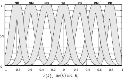
e k e k T + − ∆ = (41)

The speed errors, their variation and the control signalKi_{are chosen to be Gaussian identical}

shapes as indicated in Figure 6.

They are quantized into seven levels represented by a set of linguistic variables which are: negative big (NB), negative medium (NM), negative small (NS), zero (ZE), positive small (PS), positive medium (PM) and positive big (PB).

Fig.6. Type-2 fuzzy membership functions of the speed error, their variation and the control signalK_i

Table 1 show the linguist rules used in the IT2FGAIP Controller. Table 1. Fuzzy tuning rules forK_i [24]

∆e k( ) e k( ) NB NM NS ZE PS PM PB NB NB NB NB NM NS NVS ZE NM NB NB NM NS NVS ZE PVS NS NB NM NS NVS ZE PVS PS ZE NM NS NVS ZE PVS PS PM PS NS NVS ZE PVS PS PM PB PM NVS ZE PVS PS PM PB PB PB ZE PVS PS PM PB PB PB 0.5 ( ) e k , ∆e k( )and K i -1 -0.8 -0.6 -0.4 -0.2 0 0.2 0.4 0.6 0.8 1 0 1 NM NB NS ZE PS PM PB

The processed surface is shown in Figure 6

Fig.7. Surface for the gainK_i

5. RESULTS AND DISCUSSION

Several simulations have been run using the Matlab and Simulink® software in order to validate the theoretical results.

The IP and IT2FGAIP controllers in a DSFOC of DFIM are used as presented in Figure 1. In this section, simulations results are presented to illustrate the performance and robustness of proposed controls law, the IT2FGAIP applied to the DFIM with the speed control. The DFIM used in this work is a 0.8 KW, whose nominal parameters are reported in the table 2.

Table 2. Parameters of the DFIM. [12]

Definition Symbol Value

DFIM Mechanical Power Pw 4 kW

Stator voltage U_sn 380 V

rotor voltage Urn 220 V

Nominal current In 3.8/2.2 A

Nominal mechanical speed Ωn 1420 rpm

Nominal stator and rotor frequencies

ω

sn 50 Hz

Pole pairs number P 2

rotor resistance Rr 0.904 Ω

Stator self inductance Ls 0.414 H

rotor self inductance Lr 0.0556 H

mutual inductance M 0.126 H

Moment of inertia J 0.01 Kg.m2

friction coefficient f 0.00 IS

The speed and flux regulation performance of the proposed the IT2FGAIP is checked in terms of load torque variations. The motor is operated at 157 rad/s under no load and a load disturbance torque (5 N.m) is suddenly applied at t=0.6s and eliminated at t=1.6s (-5 N.m), and the rotor resistance variations (increase at 100 % of nominal value rotor resistance), while the other parameters are held constant.

5.1. Simulation results of vector control by direct stator flux orientation

The responses of speed, torque, stator flux and rotor current are shown in Figures 8-11.

0 0.5 1 1.5 2 -20 0 20 40 60 80 100 120 140 160 180 Time (s) S p e e d ( ra d /s ) Desierd

Vector control by direct stator flux orientation

0 0.5 1 1.5 2 -5 0 5 10 15 20 Time (s) T o rq u e ( N .m ) Torque Cr

Fig.9. Result of Torque under a load Cr=5 N.m in the interval [0,6 Sec-1,6 Sec]

0 0.5 1 1.5 2 -0.5 0 0.5 1 Time (s) S ta to r F lu x ( W b ) Flux-sd Flux-sq

Fig.10. Result of Stator flux under a load Cr=5 N.m in the interval [0,6 Sec-1,6 Sec]

0 0.5 1 1.5 2 -40 -30 -20 -10 0 10 20 30 Time (s) R o to r C u rr e n t (A )

5.2. Simulation results of IT2FGAIP

The responses of speed, torque, stator flux, rotor current and gain Ki _{are shown in Figures}

12-16; the IT2FGAIP shows the good performances to achieve tracking of the desired trajectory.

At these change of load, the IT2FGAIP throw-outs the load disturbance very rapidly with no overshoot and with a negligible static error as can be seen in the response of speed (see Figure 12). The decoupling of torque-flux is maintained in permanent mode. We can see the control is robust from the point of view load variation.

0 0.5 1 1.5 2 -20 0 20 40 60 80 100 120 140 160 180 Time (s) S p e e d ( ra d /s ) Desired IT2FGAIP

Fig.12. Result of speed under a load Cr=5 N.m in the interval [0,6 Sec-1,6 Sec]

0 0.5 1 1.5 2 -5 0 5 10 15 20 25 30 Time (s) T o rq u e ( N .m ) Torque Cr

0 0.5 1 1.5 2 -0.4 -0.2 0 0.2 0.4 0.6 0.8 1 Time (s) S ta to r F lu x ( W b ) Flux-sd Flux-sq

Fig.14. Result of Stator flux under a load Cr=5 N.m in the interval [0,6 Sec-1,6 Sec]

0 0.5 1 1.5 2 -50 -40 -30 -20 -10 0 10 20 30 40 50 60 Time (s) R o to r C u rr e n t (A )

Fig.15. Result of Rotor current under a load Cr=5 N.m in the interval [0,6 Sec-1,6 Sec]

0 0.5 1 1.5 2 0 2 4 6 8 10 12 14 16 18 20 Time (s) A d a p ti v e G a in K I

It can be seen in Figure 16 that after the torque occurs, the gain Ki increased to help the

recovery process.

In order to compare the performance of The IT2FGAIP controller with another controller in the similar test, the Figure 17 shows the simulated results comparison of conventional IP (Integral Proportional) and The IT2FGAIP controller of speed control below load and resistance variation.

The IT2FGAIP controller based drive system can handle the rapid change in load torque without overshoot and undershoot and steady state error, whereas the IP controller has steady state error and the response is not as fast as compared to The Fuzzy Gain Adaptive IP controller. Thus the proposed controller has been found superior to the conventional IP controller. 0 0.5 1 1.5 2 0 20 40 60 80 100 120 140 160 180 Time (s) S p e e d ( ra d /s ) 0.6 0.7 0.8 0.9 150 155 160 Desired

Vector control by direct stator flux orientation IT2FGAIP

ZOOM

Fig.17. Simulated results comparison of IT2FGAIP and vector control by direct stator flux orientation of speed control of DFIM under load variation with zoom in the interval [0,6

Sec-0.9 Sec] under a load Cr=5 N.m 6. CONCLUSION

In this paper, the speed regulation of DFIM with two controllers, traditional IP and IT2FGAIP controller has been designed and simulated. The comparative study shows that the IT2FGAIP controller can be improve the performances of speed of the DFIM control. The simulation results have confirmed the efficiency of the IT2FGAIP controller for different working conditions. The results show that the IT2FGAIP controller has good performance, and it is robust against exterior perturbations.

7. REFERENCES

[1] Vidal P. E. Commande non-linéaire d'une machine asynchrone à double Alimentation, Dept, of Elect, Eng. National Polytechnic Institute of Toulouse, France, 2004.

[2] Salloum G. Contribution à la commande robuste de la machine asynchrone à double alimentation, Dept, of Elect, Eng. National Polytechnic Institute of Toulouse, France, 2007. [3] Vicatos M. S. and Tegopoulos J. A. IEEE Trans. on Energy Conversion. June 2003, 18(2)

225-230, doi:10.1109/TEC.2003.811732.

[4] Bekakra Y., Ben attous D. Acta Electrotechnica et Informatica. 2010, 10(4), 75-81.

[5] Prescott J. C., Raju B.P. Proceedings of the IEE.The Institute of Electrical Engineers

Monograph. 1958, 105(7), 319-330, doi:10.1049/pi-c.1958.0040.

[6] Blaschke F. Siemens Review. 1972, 34(5), 217-219.

[7] Chaari M.,Soltani M.,Gossa M. International Journal of Sciences and Techniques of Automatic control & computer engineering IJ-STA, December 2007, 1(2),196-212.

[8] Bekakra Y., Ben Attous D. Fuzzy sliding mode controller for doubly fed induction motor speed control. J Fundam Appl Sci. 2010, 2(2), 272-287.

[9] Hebert L. X. and Tang Y. IEEE Trans. Power Electronics. September 1997, 12(5),

772-778, doi:10.1109/63.622994.

[10] Harbouche Y., Khettache L., Abdessemed R. Asian Journal of Information

Technology, 2007, 6(3), 362-368.

[11] Ben Attous D. and Bekakra Y. International Journal on Electrical Engineering and Informatics, 2010, 2(3), 179-191.

[12] Benalia L. Prof. Moulay Tahar Lamchich (Ed.), InTech. 2011, pp.113-126, doi: 10.5772/15887.

[13] Machmoum M., Poitiers F., Moreau L., Zaim M. E., Le- doeuff E. Etude d’éolienne à vitesse variable basées sur des machines asynchrones (MAS-MADA), GE44, Polytechnic

Institute of Nantes, France, 2003.

[14] Farrokh payam A., Jalalifar M. Robust speed sensorless control of doubly-fed induction machine based on input-output feedback linearization control using a sliding-mode observe, PEDES 2006,International conference on power electronics, drives and energy systems

December 12 -15,India,2006.

[15] Mendel J. M. Computational Intelligence Magazine. IEEE, 2007, 2(1), 72-73, doi: 10.1109/MCI.2007.357196.

[16] Castillo O., Melin P. Information Siences, 2014, 279, 615-631, doi:

10.1016/j.ins.2014.04.015.

[17] Ezziani N. Commande adaptative floue backstepping d’une machine asynchrone avec et sans capteur mecanique, automatic and signal processing, Reims University, France, Avril 2010.

[18] Beirami H., Zerafat M. M. Transactions of Mechanical Engineering, 2015, 39(M1), 113-129.

[19] Zadeh L.A. Information Sciences, 1975, 8(3), 199-249, doi :

10.1016/0020-0255(75)90036-5

[20] John R.I. and Coupland S. IEEE Computational Intelligence Magazine, 2007, 2(1), 57-62,

doi:10.1109/MCI.2007.357194.

[21] Mendel J. M., John R. I., Liu F. IEEE Trans. Fuzzy Syst, 2006, 14(6), 808-818, doi: 10.1109/TFUZZ.2006.879986.

[22] Hagras H. A. IEEE Trans. Fuzzy Syst, 2004, 12(4), 524-539, doi: 10.1109/TFUZZ.2004.832538.

[23] Liang Q. and Mendel J. M. IEEE Trans. Fuzzy Syst, 2000, 8(5), 535-550.

[24] Barkati S., Berkouk E. M., Boucherit M. S. Electr Eng, 2008, 90(5), 347-359, doi: 10.1007/s00202-007-0087-x.

How to cite this article:

Loukal K and Benalia L. Interval type-2 fuzzy gain-adaptive controller of a doubly fed