HAL Id: hal-01657086
https://hal-polytechnique.archives-ouvertes.fr/hal-01657086
Submitted on 6 Dec 2017
HAL is a multi-disciplinary open access
archive for the deposit and dissemination of
sci-entific research documents, whether they are
pub-lished or not. The documents may come from
teaching and research institutions in France or
abroad, or from public or private research centers.
L’archive ouverte pluridisciplinaire HAL, est
destinée au dépôt et à la diffusion de documents
scientifiques de niveau recherche, publiés ou non,
émanant des établissements d’enseignement et de
recherche français ou étrangers, des laboratoires
publics ou privés.
Two scale homogenization of a row of locally resonant
inclusions - the case of anti-plane shear waves
Kim Pham, Agnes Maurel, Jean-Jacques Marigo
To cite this version:
Kim Pham, Agnes Maurel, Jean-Jacques Marigo. Two scale homogenization of a row of locally resonant
inclusions - the case of anti-plane shear waves. Journal of the Mechanics and Physics of Solids, Elsevier,
2017, 106, pp.80-94. �10.1016/j.jmps.2017.05.001�. �hal-01657086�
Two scale homogenization of a row of locally resonant inclusions
- the case of anti-plane shear waves
Kim Pham
IMSIA, ENSTA ParisTech - CNRS - EDF - CEA, Universit Paris-Saclay, 828 Bd des Marchaux, 91732 Palaiseau, France
Agn`es Maurel
Institut Langevin, ESPCI ParisTech, CNRS, 1 rue Jussieu, Paris 75005, France
Jean-Jacques Marigo
Laboratoire de M´ecanique des solides, Ecole Polytechnique, Route de Saclay, 91120 Palaiseau, France
Abstract
We present a homogenization model for a single row of locally resonant inclusions. The reso-nances, of the Mie type, result from a high contrast in the shear modulus between the inclusions and the elastic matrix. The presented homogenization model is based on a matched asymptotic expansion technique; it slightly di↵ers from the classical homogenization which applies for thick arrays with many rows of inclusions (and thick means large compared to the wavelength in the matrix). Instead of the e↵ective bulk parameters found in the classical homogenization, we end up with interface parameters entering in jump conditions for the displacement and for the nor-mal stress; among these parameters, one is frequency dependent and encapsulates the resonant behavior of the inclusions. Our homogenized model is validated by comparison with results of full wave calculations. It is shown to be efficient in the low frequency domain and accurately describes the e↵ects of the losses in the soft inclusions.
Keywords: 1. Introduction
Metamaterial structures are constructed by repeating, most often periodically, a unit cell. They may have a lattice periodicity of the same order of magnitude than the working wave-length, resulting in a structure of the crystal type; such structures present resonant behaviors due to Bragg scattering mechanism. In the 2000’s, resonant structures with subwavelength unit cells have been proposed in the context of elasticity (Liu et al., 2000) and in the context of electromag-netism (O’Brien and Pendry, 2002). In this case, the resonances are attributable to an inclusion placed in the unit cell and presenting a high contrast in its material properties with respect to the surrounding matrix. These resonances often referred to as Mie resonances occur at frequencies producing a wavelength in the inclusion comparable to the inclusion size (and this size is much Preprint submitted to Journal of the Mechanics and Physics of Solids January 12, 2017
smaller than the wavelength in the matrix). The ability of these so-called locally resonant struc-tures to forbid the wave propagation has been exhibited and the forbidden band gaps have been interpreted in terms of an e↵ective negative parameter being the mass density in elasticity (Liu et al., 2000) and the permeability in electromagnetism (O’Brien and Pendry, 2002). Since then, locally resonant materials have been intensively studied for applications including the design of efficient wave shields (Go↵aux et al., 2002; Ho et al., 2003), absorbers of small thicknesses (Gof-faux et al., 2004; Zhao et al., 2010; Brunet et al., 2013) and subwavelength waveguides (Achaoui et al., 2011; Jin et al., 2016).
Because of their subwavelength scales, homogenization approaches are well adapted to de-scribe the e↵ective properties of such structures. As primarily proposed in Liu et al. (2000) and in O’Brien and Pendry (2002), the thickness of the resonant material was large compared to any wavelength outside the inclusions so that the bulk e↵ect of this massive structure on the wave propagation was regarded. In this context, extensions of the classical homogenization to high contrast versions have been proposed in elasticity by Auriault (1994) and Auriault and Boutin (2012) and in electromagnetism by Zhikov (2000, 2005); Felbacq and Bouchitt´e (2005); Bouch-itt´e et al. (2009). These high contrast homogenizations provide e↵ective bulk parameters among which the e↵ective mass density or permeability is frequency dependent and may change in sign as a result. It is worth noting that, in the two contexts of waves, the constitutive equations being respectively the Navier equations and the Maxwell equations di↵er but the conclusions are of the same nature and conform to the expectations (we refer to ”expectations” the expected negative parameters previously obtained using retrieval methods). Note also alternative methods based on computational homogenization (Pham et al., 2013). A priori, the story should end here.
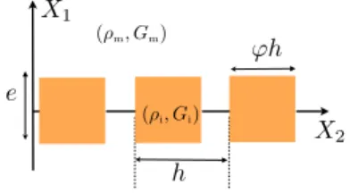
h X1 X2 e ( m, Gm) ( i, Gi)
Figure 1: The array composed of a single row of locally resonant inclusions with material properties (⇢i,Gi) embedded
in an elastic matrix with (⇢m,Gm).
However, motivated by the design of compact metamaterial devices and following the intu-itive argument that each local resonator vibrates almost like an independent unit, structures in-volving a single row of resonators or few rows have been thought, see e.g. Ho et al. (2003), Zhao et al. (2010). In this case, interrogating the bulk response of the device becomes questionable. Indeed, when the number of cells is too small, the metamaterial device is dominated by bound-ary layer e↵ects and the response of its bulk is not pertinent anymore; the failure of the e↵ective medium theories for thick structures has been illustrated recently in Lapine et al. (2016) and in Marigo and Maurel (2016a), Marigo and Maurel (2016b) (non resonant structures were consid-ered in these references). Homogenization approaches able to handle such thin structures have been developed originally in the context of solid mechanics (Sanchez-Palencia, 1987; Bakhvalov and Panasenko, 1989; Marigo and Pideri, 2011). In the context of wave propagation, they have been adapted in geophysics (Capdeville and Marigo, 2013), in acoustics (Bonnet-Bendhia et al., 2004; Marigo and Maurel, 2016a,b) and in electromagnetism (Delourme et al., 2012; Delourme,
2015; Maurel et al., 2016; Marigo and Maurel, 2016c), see also (Felbacq, 2015). Here, we extend these works to the case of an array composed of a single row of locally resonant inclusions (Fig. 1). We restrict ourselves to the case of two dimensional shear wave propagation, which reduces our conclusions to a scalar case but make them applicable to the case of polarized electromag-netic waves as considered in Felbacq and Bouchitt´e (2005); note that the extension to the three dimensional case is quite easy in elasticity but more tricky in electromagnetism.
The homogenized model is presented in Section 2; it basically relies on the same ingredients than the classical homogenization, a two scale method and an asymptotic expansion of the solu-tion. The solution is expressed in a rescaled, or renormalized, structure accounting for a small parameter
⌘⌘ kh ⌧ 1, (1)
(k is the wavenumber in the matrix and h the spacing between the inclusions in the row) and accounting for the high contrast in the shear modulus; this latter has to scale as 1/⌘2to produce
wavelengths in the inclusions of the order of h. In addition, it accounts for the small thickness of the device and this is done by using two di↵erent expansions near and far from the array, which are connected using so-called matching conditions. The homogenization is conduced up to O(⌘2) and it makes e↵ective interface parameters to appear, which enter in jump conditions on
the displacement and on the normal stress across an equivalent interface whose interior region is disregarded (Fig. 2). In the present case, we obtain six interface parameters among which one is frequency dependent. The homogenized problem is validated in Section 3 by comparison with full wave calculations in two cases of interest: first we inspect the scattering by such thin metafilms for a plane wave at oblique incidence, afterwards the ability of the array to support guided waves is regarded. In both cases, the e↵ect of losses within the inclusions is considered (the e↵ect of the losses in the matrix is trivial and it is disregarded). The homogenized problem can be solved explicitly, yielding the scattering coefficients and of the dispersion relation of the guided waves, respectively in the two problems.
X1
X2
e
jump cond.
Figure 2: In the homogenized problem, the row of inclusions is replaced by an equivalent thick interface. Across the interface, jump conditions apply, Eq. (3), and the region inside the interface |X1| < e/2 is disregarded.
2. The real and the homogenized problems
We consider two dimensional shear waves propagating in an elastic matrix containing a single row of periodically located elastic inclusions with spacing h and thickness e = O(h) (Fig. 1). The mass density ⇢ and the shear modulus G are spatially varying parameters being piecewise
constants; in the matrix, ⇢(X) = ⇢m, G(X) = Gmand in the inclusions ⇢(X) = ⇢iG(X) = Gi. In the
harmonic regime, the elastic displacement U has a time dependence e i!twith ! the frequency
(the time dependence will be omitted in the following), and the wave equation reads 8
>>>< >>>:
div⌃ + ⇢!2U = 0, ⌃ = G rU,
with U and ⌃.n being continuous at each interface matrix/inclusion. (2) With k = !p⇢m/Gm the wavenumber in the matrix, the low frequency regime concerns the
frequency range for which ⌘ ⌘ kh ⌧ 1. Next, we are interested in resonances in the inclusions and this is possible if kih = O(1), with ki= !
p
⇢i/Githe wavenumber in the inclusions. We shall
consider a low contrast in the mass density ⇢i/⇢m=O(1) and a high contrast in the shear modulus
with Gi= ⌘2G0and G0/Gm=O(1).
High contrasts in the shear moduli are easy to obtain; rubbers and silicon rubbers o↵er a variety of shear modulus values ranging from 104to 107Pa with roughly the same density ⇢ '
1300 kg.m 3, see e.g. Lai et al. (2011), and obviously sti↵er materials exist with a similar mass
density. In electromagnetism for transverse magnetic polarization (the magnetic field plays the role of U in (2)), the situation is the same. In this case, the permeability plays the role of ⇢ and the permittivity plays the role of G; therefore, non magnetic dielectric materials o↵er a class of materials with the same permeability (the one of the vacuum) and possibly high contrasts in the permittivity, see e.g. Campione et al. (2012). The story is di↵erent for acoustic waves in fluids; the propagation of these longitudinal waves is described by the linearized Euler equations, yielding div⇣rP
⇢
⌘
+!B2P = 0, with P the acoustic pressure, ⇢ the mass density and B = ⇢c2the bulk modulus. However, if a high contrast in the mass density can be obtained, for instance between gases and liquids, the sound speeds are of the same order of magnitude in most fluids; it results that the wavelengths cannot be tuned di↵erently by playing on the material properties (B and ⇢ scale the same). This particularity has practical consequences when comparing the acoustic metamaterials and their electromagnetic/elastic counterparts (Cordero et al., 2015; Mercier et al., 2015) and other strategies to obtain local resonances have to be found; these can consist in using elastic inclusions in liquids (Ding et al., 2007) or exploiting other type of resonances, for instance Minnaert resonances (Bretagne et al., 2011) or the resonances of the Helmholtz type (Guenneau et al., 2007; Elford et al., 2010).
We come back to our problem and its homogenized counterpart. We shall see that the row of inclusions can be described by an equivalent layer, or an enlarged interface, with the same thickness and associated to jump conditions relating the values of the homogenized field on its both sides (Fig. 2). Specifically, for inclusions with simple symmetry shape, the homogenized problem consists in solving
8 >>>>> >>>>> >>>< >>>>> >>>>> >>>: Uh+k2Uh=0, |X 1| >2e, Jump conditions 8 >>>>> >>>< >>>>> >>>: JUh Ke=hB @Uh @X1, s@Uh @X1 { e =hS@ 2Uh @X2 1 +hC @ 2Uh @X2 2 hD(k) k 2 Uh, (3)
where we defined, for any field f , J f Ke⌘ f+ f and f ⌘ ( f++f )/2, with f±⌘ f (±e/2, X2).
The e↵ective parameters (B, C, S) depend only on the geometry of the inclusions while D(k) has an additional dependence on the frequency and it is the parameter which encapsulates the possible resonances of the Mie type. For instance, for rectangular shape of inclusion, as we shall consider in the numerical example, we have
8 >>>>> >>>>> >< >>>>> >>>>> >:
B = 1 'e/h ⇡2log sin⇡(1 ') 2 ! , C ' he(1 ') ⇡ 8(1 ')2, S = eh(1 ') , (4)
where h' is the length of the rectangular inclusion along X2(see forthcoming Section 3), and
8 >>>>> >>>< >>>>> >>>: D(k) = ⇢i ⇢m e' h 2 66666 41 X n ↵2n k 2 i k2 i k2i,n 3 77777 5 , with n = (n1,n2), k2i,n⌘✓ n1 ⇡ e ◆2 + n2⇡ h' !2 and ↵n ⌘ 8 ⇡2n1n2. (5)
In the following, a more general form of the homogenized problem is derived for non sym-metric inclusions, Eqs. (44) with basically the same conclusion. Note that the above system does not interrogate the region |X1| < e/2, where the solution does not need to be defined.
Finally, the problems (2) and (3) have to be associated to boundary conditions at |X| ! +1. These boundary conditions are in general radiation conditions of the Sommerfeld type, which select outgoing scattered waves once the incident wave has been defined. We do not need to specify them for the time being.
2.1. The rescaled outer and inner problems
To begin with, the real problem (2) is written using the non-dimensional coordinatesx ⌘ kX, with k the wavenumber in the matrix (k2= ⇢
m!2/Gm). We define the fields
u(x) ⌘ U(X), (x) ⌘ kG1
m
⌃(X), (6)
and the spatially dependent parameters a(x) ⌘ ⇢(X)⇢
m
, b(x) ⌘ G(X) Gm
, (7)
being the relative mass density and shear modulus. Thus, we have a(x) = 1 = b(x) in the matrix, and with Gi= ⌘2G0, a(x) = ai= ⇢i/⇢mand b(x) = bi= ⌘2b0in the inclusions (with b0 =G0/Gm).
Inx coordinate, the system (2) reads 8
>>>>< >>>>:
div + au = 0, =bru,
u and .n continuous at the inclusions/matrix interface.
(8a) (8b) (8c) 5
Next, we shall use two systems of coordinates,x = kX and y ⌘ X/h (whence y = x/⌘); they account respectively for slow variations of the wavefield (the macro scale being the wavelength in the matrix) and for the rapid variations of the wavefield (the micro scale associated to the subwavelength structure of the row). Obviously, the dependance of the fields (u, ) onx and y is pertinent or not, depending on how close we are to the inclusions. Sufficiently far away from the row, only the propagating field is associated to variations of u and on the scale of the wavelength 1/k; thus, onlyx is needed. In the near field, the wavefield is more complex since it experiences (i) rapid variations of the evanescent field, being associated to all the scales between 1/k and h and (ii) slow variations in 1/k, associated to the propagating field along x2(for instance
through the condition of the quasi-periodicity for plane waves). Thus, the rapid variations in the near field problem are handled by the coordinatesy and to account for the slow variations, we keep x2as additional coordinate.
From what has been said, the expansions of the solution are written di↵erently in the two regions; we use in the far field, also named outer region, the following expansions
8 >>>< >>>: u = u0(x) + ⌘u1(x) + . . . , = 0(x) + ⌘ 1(x) + . . . (9) and in the near field, or inner region,
in ⌦\⌦i 8 >>>< >>>: u = v0(y, x2) + ⌘v1(y, x2) + . . . , =⌧0(y, x2) + ⌘⌧1(y, x2) . . . in ⌦i 8 >>>< >>>: u = v0 i(y, x2) + ⌘v1i(y, x2) + . . . , =⌧0i(y, x2) + ⌘⌧1i(y, x2) . . . (10)
(Fig. 3 shows the rescaled inner domains ⌦ and ⌦iiny coordinates). As in the classical
homog-enization, the fields vnand ⌧n, n = 0, . . . , are assumed to be periodic with respect y
2 2 (0, 1) and
this is not meaningless in the present context since the condition of pseudo-periodicity is handled by the variables x2(thus, we recognize Floquet type solutions for (vn,⌧n)).
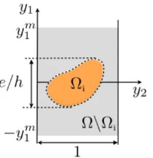
y1 y2 1 e/h y1m y1m i \ i
Figure 3: Rescaled domains ⌦iand ⌦. In ⌦,y 2 ( ym1,ym1)⇥(0, 1) and in practice, the limit ym1 ! +1 will be considered.
In the following, (8) will be written at each order using the di↵erential operators 8
>>>< >>>:
r ! rx, in the outer region,
r ! 1⌘ry+e2 @x@
2, in the inner region.
(11) 6
In the outer region, (8a)-(8b) apply at each order (with a(x) = 1 = b(x)). We shall need the orders n = 0 and 1, for which
(
div n+un=0, n=run.
(12a) (12b) In the inner regions ⌦\⌦i and ⌦i, (8) takes di↵erent forms at each order using (11) with a
and b given by (
a(y) = 1 = b(y), in ⌦\⌦i,
a(y) = ai, b(y) = ⌘2b0, in ⌦i. (13)
2.2. Boundary conditions and matching conditions between the inner and outer solutions By construction, the inclusions are seen by the inner solution only; the continuity of the displacement and of the normal stress at the interface @⌦iapply at each order, with
vn
|@⌦i =vni|@⌦i, and ⌧
n.n
|@⌦i=⌧ni.n|@⌦i,n = 0, 1, . . . (14)
Reversely, the boundary conditions at |x| ! +1 apply to the outer solution only. It follows that boundary conditions for |y1| ! +1 are missing in the inner problem and they are missing for
x1 ! 0±in the outer problem. These conditions are provided by the matching conditions; they
ensure the continuity of u and in an intermediate region where the evanescent field can be considered as negligible. It is y1 ! ±1 for the near field solution and it is x1 ! 0± for the
far field solution. Owing to the Taylor expansion, u0(x1,x2) = u0(0, x2) + x1@x
1u0(0, x2) + · · · =
u0(0, x2) + ⌘y1@x
1u0(0, x2) + . . . (same for 0), we get at order 0
8 >>>>< >>>>: u0(0±,x2) = v0(±1, y 2,x2), 0(0±,x 2) = ⌧0(±1, y2,x2), (15a) (15b) and at order 1, 8 >>>>> >>>>> < >>>>> >>>>> : u1(0±,x 2) = limy 1!±1 " v1(y, x 2) y1 @u 0 @x1(0 ±,x 2) # , 1(0±,x2) = lim y1!±1 " ⌧1(y, x2) y1 @ 0 @x1(0 ±,x2) # . (16a) (16b) The boundary conditions for the outer solution at x1 =0±will provide the jump conditions
that we are looking for, and from (15)-(16), they require the inner solution to be known. Also, we shall see that relevant jump conditions require to go at order 1, and the orders 0 and 1 refer to the order of the outer solution.
2.3. The jump conditions at order 0
We start with the inner problem. In ⌦\⌦i, Eqs. (8a)-(8b) at order ⌘ 1along with (13) give
ryv0=0, divy⌧0=0, in ⌦\⌦i, (17)
and in ⌦i, (8b) at order ⌘0and (13) give
⌧0i =0, in ⌦i. (18)
The first equation of (17) tells us that v0does not depend on y, and we deduce from the matching
condition (15a) that u0is continuous at x
1=0 with
v0(x
2) = u0(0±,x2). (19)
Now, we integrate over ⌦\⌦ithe relation divy⌧0=0 from (17). Owing to (i) ⌧0.n|@⌦i =⌧0i.n|@⌦i =
0 from (14) and (18), and owing to (ii) the periodicity of ⌧0with respect to y
2, we get
Z
dy2 ⌧01(ym1,y2,x2) =
Z
dy2⌧01( ym1,y2,x2),
(when integrating over y2, we consider implicitly y2 2 (0, 1)). Taking the limit ym1 ! +1, the
matching conditions (15b) gives the continuity of the normal component to the interface of 0,
namely
0
1(0+,x2) = 01(0 , x2), (20)
(note that the matching conditions (15b) have been integrated with respect to y22 (0, 1)). At this
leading order, the row of inclusions is transparent for the wave and we shall consider the next order to get the e↵ect of the array.
2.4. The jump conditions at order 1
2.4.1. The Neumann elementary problems and the jump condition on u1
The jump condition on u1requires only the solution v1in ⌦\⌦
ito be determined and we shall
see that v1is independent of the solution in ⌦
iat this order. The problem satisfied by v1reads
in ⌦\⌦i 8 >>>>> >>>< >>>>> >>>: divy⌧0 =0, ⌧0=ryv1+@u 0 @x2(0, x2)e2, ⌧0.n|@⌦i =0, lim y1!±1⌧ 0=@u0 @x1(0, x2)e1+ @u0 @x2(0, x2)e2. (21)
In the above system, the equilibrium and the constitutive relation followed from (17) and (8b) at order ⌘0along with (13) and v0(x
2) = u0(0, x2), Eq. (19). The boundary condition on @⌦iis
deduced from (14) using (18). Finally, the limit values for y1 ! ±1 are given by the matching
conditions (15b) and provide the last conditions needed to solve the problem on v1 up to a term
which depends only on x2. The problem on v1appears to be linear with respect to @x1u0(0, x2)
and @x2u0(0, x2). Specifically, let us write
v1(y, x 2) =@u 0 @x1(0, x2)V (1)(y) +@u0 @x2(0, x2)V (2)(y) + ˜v(x 2). (22)
It is easy to see that v1is solution of the problem if V(i), i = 1, 2 satisfy
8 >>>>> >>>< >>>>> >>>: V(1)=0, rV(1).n |@⌦i =0, lim y1!±1rV (1)=e 1, 8 >>>>> >>>< >>>>> >>>: V(2)=0, ⇥rV(2)+e 2⇤.n|@⌦i=0, lim y1!±1rV (2)=0. (23) 8
These two elementary Neumann problems are independent of the incident wave u0, contrary to v1
in (21). Incidentally, they are the same as those encountered when considering a row of cracks or of voids (Marigo and Maurel, 2016a,c); thus, it is clear that they will not encapsulate the possible resonances of the soft inclusions.
From (23), V(1)and V(2), being defined up to a constant, can be chosen in the form
V(1)(y) = 8 >>< >>: y1 +V(1) ev(y), y1<0 y1+B1+Vev(1)(y), y1>0, V(2)(y) = 8 >>< >>: V (2) ev (y), y1 <0 B2+Vev(2)(y), y1 >0, (24) where V(i)
ev(y), i = 1, 2 are evanescent fields, vanishing at y1! ±1. Thus, B1=ylim 1!+1(V (1) ev((y)) y1) and B2= lim y1!+1V (2)
ev((y)), with Bibeing constant values (i = 1, 2). Now, it is sufficient to use
the matching condition (16a) to get q u1y 0=B1 @u0 @x1(0, x2) + B2 @u0 @x2(0, x2), (25)
which provides the first jump condition written here for u1 across a zero thickness interface at
x1=0.
2.4.2. The resonant Dirichlet elementary problem and the jump condition on 1
The derivation of the jump condition on 1is more demanding and requires the solution v0
i
to be determined in ⌦i. The solution v0i satisfies
in ⌦i 8 >>>< >>>: divy⌧1i +aiv0i =0, ⌧1i =b0ryv0i, v0 i|@⌦i =u 0(0, x 2). (26) We used (8a) at the order ⌘0and (8b) at the order ⌘1, and in both cases, we also used that ⌧0
i =0,
Eq. (18). The boundary condition is given by (14), with (19). This problem is of the Dirichlet type, and it can be solved by noting the linearity of the solution with respect to u0(0, x
2). As for
the Neumann elementary problems, defining v0
i(y, x2) = u0(0, x2)Vk(y), (27)
v0
i will be solution of (26) as soon as Vkis the solution of the Dirichlet elementary problem
in ⌦i 8 >>>< >>>: Vk+ 2Vk=0, Vk|@⌦i=1, (28) with 2 ⌘ a
i/b0. It is worth noting that depends implicitly on the frequency or equivalently
to the wavenumber k in the matrix, with 2 = (⇢
i/⇢m)(Gm/Gi) (kh)2 once coming back to the
physical quantities; in other words, is the rescaled version of ki, with
=kih. (29)
For frequencies di↵erent of the eigenfrequencies nof (28), the solution is unique and reads
Vk(y) = 1 X n vn 2 2 2n Pn(y), (30) 9
where the Pn(y) are the eigenfunctions associated to the eigenvalues n2and vnis the projection
of Pnon 1 (Appendix A).
We can now determine the jump in 1
1. We start with (8a) at order ⌘0in ⌦\⌦i, integrated on
⌦\⌦i, namely Z ⌦\⌦i dy 2 66664divy⌧1+ @⌧02 @x2 +u 0(0, x 2) 3 77775 = 0, (31) where we used (19). Let us inspect the three integrals in (31); the first integralR⌦\⌦
idy divy⌧
1
can be expressed as follow Z ⌦\⌦i dy divy⌧1= Z dy2 ⌧11|ym 1 ⌧ 1 1| ym 1 + Z @⌦i ⌧1i.n, (32) where we used the periodicity of ⌧1 with respect to y2 and the continuity relation ⌧1.n
|@⌦i =
⌧1i.n|@⌦i, Eq. (14). The second term in (32) can be expressed as a function of Vkby integrating
the relation divy⌧1i +aiv0i =0 (from (26)) over ⌦i. This leads to
R @⌦i⌧ 1 i.n = ai R ⌦iv 0 i (withn being
inward), and with v0
i in (27), to Z @⌦i ⌧1i.n = aiu0(0, x2) Z ⌦i dy Vk.
The second integral in (31) reads Z ⌦\⌦i dy @⌧02 @x2 = @2u0 @x1@x2(0, x2) Z ⌦\⌦i dy @V(1) @y2 + @2u0 @x2 2 (0, x2) Z ⌦\⌦i dy " @V(2) @y2 +1 # , (33) where we used that ⌧0
2 =
h
@y2v1+ @x2u0(0, x2)
i
, from (21), with v1 given by (22). Finally, the
third integral in (31), with u0(0, x
2) being independent ofy, simply reads
Z ⌦\⌦i dy u0(0, x 2) = u0(0, x2)⇣2ym1 Si ⌘ , (34)
where Siand (2ym1 Si) are the dimensionless surfaces (iny coordinates) of ⌦iand ⌦\⌦i,
respec-tively. Collecting the three integrals (32)-(34), we get Z dy2 ⌧11|ym 1 ⌧ 1 1| ym 1 2y m 1 @ 01 @x1(0, x2) = Si @2u0 @x2 1 (0, x2) aiu0(0, x2) Z ⌦i Vk @2u0 @x1@x2(0, x2) Z ⌦\⌦i @V(1) @y2 @2u0 @x2 2 (0, x2) Z ⌦\⌦i @V(2) @y2 , (35) where we have used @2
x2u
0+u0 = @2 x1u
0 = @
x1 01 from (12). It is now sufficient to take the
limit ym
1 ! +1 in (36) (integrated over y2 2 (0, 1)), with
⌧11|ym 1 y m 1@x1 01(0, x2) ! 11(0, x2) and⌧11| ym 1 +y m
1@x1 01(0, x2) ! 11(0, x2), to get the jump of @x1u1= 1
s@u1 @x1 { 0 = Si @2u0 @x2 1 (0, x2) + C1 @ 2u0 @x1@x2(0, x2) + C2 @2u0 @x2 2 (0, x2) D(k)u0(0, x2), (36) 10
where we have defined the dimensionless parameters Ci⌘ Z ⌦\⌦i dy @V(i) @y2(y), i = 1, 2, and D(k) ⌘ ⇢i ⇢m Z ⌦i dy Vk(y). (37)
This provides the second jump condition, and as (25), it is expressed across a zero thickness interface at x1=0.
2.5. The homogenized problem and the associated final jump conditions
The final jump conditions will be written, from (25) and (36), in a di↵erent and equivalent form up to O(⌘2). From (9), we have
u = u0+ ⌘u1+O(⌘2), (38)
and, from (12), (25) and (36), u satisfies 8 >>>>> >>>>> >>< >>>>> >>>>> >>: u + u = 0, JuK0= ⌘B1 @u 0 @x1(0, x2) + ⌘B2 @u0 @x2(0, x2) + O(⌘ 2), s@u @x1 { 0 = ⌘Si @2u0 @x2 1 (0, x2) + ⌘C1 @ 2u0 @x1@x2(0, x2) + ⌘C2 @2u0 @x2 2 (0, x2) ⌘D(k)u0(0, x2) + O(⌘2). (39) As written in (39), the homogenized problem could be solved using an iterative process: first, compute u0and its spatial derivatives along x
1 =0 to get the right hand side terms of the jump
conditions (compute also the parameters Bi, Ci, i = 1, 2 and D), then compute u up to O(⌘2). It
has been discussed in David et al. (2012) that such resolution is not satisfactory. Firstly because it requires the numerical computation of spatial derivatives of the fields at x1 = 0 which is
demanding for continuous fields, as u0, and may become technically involved for discontinuous
fields, as u1which will be required for the jump condition on u2(and this remark is not incidental
in the present case, see Section 4). Instead, David et al. (2012) propose the construction of a unique problem for a field uhadmitting the same expansion as u0+ ⌘u1up to O(⌘2) (and thus, the
same expansion as the real field u). Besides, it is stressed that this problem admits a variational formulation, which allows to define an energy being the sum of the usual elastic energy and a surface energy supported by the equivalent interface. Also, it has been shown that it is preferable to express the jump conditions across an enlarged version of the interface (Fig. 4). In Delourme et al. (2012), this is done to ensure stability properties of the obtained conditions with respect to ⌘ and with respect to the frequency; in Marigo and Maurel (2016a), this is done in order to ensure a positive energy supported by the interface, see also Marigo et al. (2016). In both cases, an important consequence is to get a formulation suitable for numerical implementations (Lombard et al., 2016). The two above mentioned aspects will be addressed. First, we define an enlarged version of the jumps and associated average value for any field f (x1,x2)
J f K⌘ f+ f , f ⌘ 12⇥ f + f+⇤, with f± = f ±ke 2,x2 ! . (40)
Now, we use the Taylor expansion u0 ±ke 2 ,x2 ! =u0(0±,x2) ± ⌘2he @u 0 @x1 ± ke 2,x2 ! +O(⌘2), (41) 11
where we used e/h = O(1), and from (39), we get the jump condition JuK = ⌘✓B1+e h ◆ @u @x1 + ⌘B2 @u @x2 +O(⌘ 2), (42)
(and the same is done to get the jump of J@u/@x1K).
x2
jump cond. x1
x2 e
final jump cond. x1
Figure 4: (a) Initial jump conditions (39) across a zero thickness interface at x1=0, (b) Final jump conditions (3) across the enlarged interface.
Now, we define the new homogenized problem 8 >>>>> >>>>> >>>< >>>>> >>>>> >>>: uh+uh=0, Juh K = ⌘✓B1+he◆ @u h @x1 + ⌘B2 @uh @x2, s @uh @x1 { = ⌘✓ e h Si ◆ @2uh @x2 1 + ⌘C1 @ 2uh @x1@x2 + ⌘C2 @2uh @x2 2 ⌘D(k)uh. (43)
It is easy to see that uhadmits the same expansion as u up to O(⌘2) and (43) is our homogenized
problem in rescaled coordinate. It is now sufficient to come back to the real space to get the final homogenized problem consists in solving, outside the interface occupyingX 2 ( e/2, e/2) ⇥ ( 1, +1) 8 >>>>> >>>>> >>>< >>>>> >>>>> >>>: Uh+k2Uh=0, e 2 <|X1|, JUh Ke=hB01 @Uh @X1 +hB2 @Uh @X2, s@Uh @X1 { e =hS@ 2Uh @X2 1 +hC1 @ 2Uh @X1@X2 +hC2 @2Uh @X2 2 hD(k) k2Uh, (44) with B0
1 ⌘ e/h + B1, S = e/h Si(Bi, Ci, i = 1, 2 and D have been defined in (24) and (37)),
and where JFK ⌘ F(e/2, X2) F( e/2, X2) and F ⌘ 1/2 [F(e/2, X2) + F( e/2, X2)].
2.6. The case of symmetrical inclusions
In the case of inclusions being symmetric with respect to y2, the e↵ective parameters C1and
B2vanish, leading to the form in (3), with B = B01and C = C2. This is because the elementary
solutions V(1) and V(2)in (23) are respectively symmetric and antisymmetric with respect to y
2.
This implies that B2 =0 in (24) because V(2)(y1,0) = 0, and C1 =0 in (37) since @y2V(1)is odd
in y2 (thus its integral vanishes). Besides, the expressions of these parameters for rectangular
inclusions, as we shall consider in the following section, are known (Marigo and Maurel, 2016a) and they have been given in Eqs. (4); note that better estimates of (B, C) can be obtained by solving numerically the elementary problems (24) while D is obtained explicitly, see Appendix A.
3. Validation of the homogenized interface problem
In this section, we address the validity of our homogenized problem (3) with respect to the real one. This is done considering two classical problems for wave propagating in such an array of locally resonant inclusions: (i) the scattering of incident plane waves and (ii) the propagation of guided waves supported by the array. In both cases, the e↵ect of losses in the inclusions is regarded and this is relevant in view of practical applications. In the former case, the absorption resulting from the losses is known to be significant near the resonance, resulting in an efficient thin ”metamaterial absorber” able to block the wave propagation over a short distance, and short is meant when compared to the wavelength. In the latter case, the losses are unwanted since they produce energy leakage from the array along which the guided wave propagates; this may produce the suppression of the guiding e↵ect. In both cases, a theoretical prediction on the e↵ects of resonances of lossy inclusions is proposed, owing to the explicit solutions available in the homogenized problem.
h X1 X2 e ( i, Gi) h (i, Gi) ( m, Gm)
Figure 5: The array composed of a single row of rectangular locally resonant inclusions.
We shall consider an array of square, or rectangular, inclusions (Fig. 5). A contrast in the shear modulus Gm/Gi =100 with ⇢m/⇢i =1 is considered; it is a rather modest contrast which
could be obtained with soft silicon rubber inclusions in a hard silicon matrix (Lai et al., 2011). In electromagnetism, this contrat is obtained with non magnetic inclusions of TiO2 in the air
(Lanneb`ere et al., 2014). When the e↵ect of losses is regarded, only the losses in the inclusions are considered, being encapsulated in a complex value of 1/Gi = (1 + i⇠)/G0, resulting in a
complex wavenumber ki in the inclusions. The actual problem of the array of locally resonant
inclusions is solved numerically using full wave calculations (Maurel et al., 2014), and we denote Unumthe wavefield of the numerical solution. The solution of the homogenized problem satisfies
(3), with the interface parameters in (4)-(5).
3.1. Reflection, transmission and absorption of an incident plane wave
In our homogenized problem, the region |X1| < e/2 is disregarded and the wavefield satisfies
(3) for |X1| > e/2; a solution of this problem for an incident plane wave at oblique incidence ✓
reads Uh(X) = 8 >>>>> < >>>>> : h
eik(X1+e/2) cos ✓+Rhe ik(X1+e/2) cos ✓i eikX2sin ✓, X
1< e2
Theik(X1 e/2) cos ✓eikX2sin ✓, e
2 <X1,
(45) and this solution is thought to (i) satisfy the condition of pseudo periodicity Uh(X
1,X2 +h) =
Uh(X
1,X2)eik sin ✓himposed by the form of the incident wave Uinc=eik cos ✓(X1+e/2)+ik sin ✓X2, and (ii)
to satisfy the radiation condition for |X1| ! +1 of outgoing scattered waves (Uh Uinc).
Next, applying the jump conditions (3) yields the scattering coefficient 8 >>>>> >>>>> < >>>>> >>>>> : Rh= 1 2 " z1 z⇤ 1 z2 z02 z⇤ 2+z02 # , Th=1 2 " z1 z⇤ 1 +z2 z 0 2 z⇤ 2+z02 # , z1⌘ 1 + ikh2 Bcos ✓, z2⌘ cos ✓ + ikh2 h S cos2✓ +C sin2✓ +D r(k) i , z0 2= kh 2 Di, (46)
where z⇤denotes the complex conjugate of z. We used that the presence of losses in the inclusions
a↵ects only the parameter D = Dr+iDiaccording to (5), since k2i =k2i0(1 + i⇠) is complex. Note
that, near the first Mie resonance, Drand Dican be approximated by
Dr(k) ' A " 1 ↵2 1 (k2/k2 m 1) (k2/k2 m 1)2+ ⇠2 # , and Di(k) ' A↵21 ⇠ (k2/k2 m 1)2+ ⇠2 , (47) with A ⌘ e'/h and where k2
m⌘ (⇢i/G0)k2i,1is the wavenumber (being real) in the elastic matrix
producing the first, monopolar resonance in the inclusions. It is worth noting that in absence of attenuation, z0
2=0 and we recover |Rh|2+|Th|2=1 as expected.
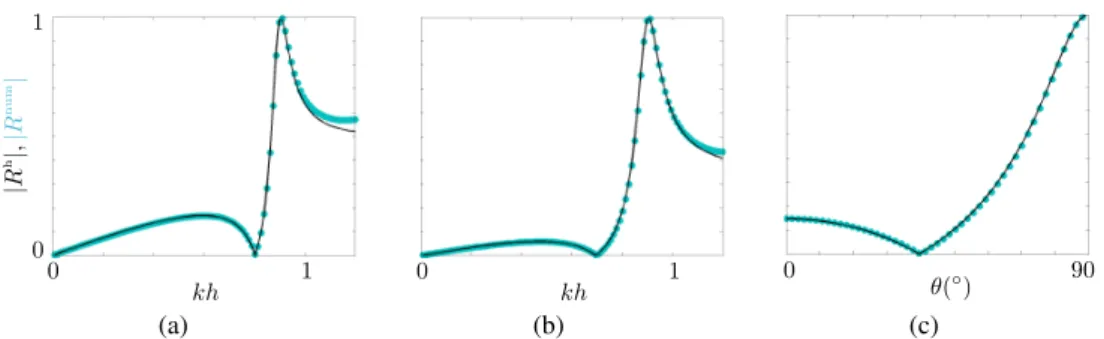
To begin with, we report in Fig. 6 the variations of the reflection coefficients in the absence of losses as a function of the dimensionless frequency kh, Rnumbeing computed numerically and Rh
from (46). In the range kh 2 [0, 1.2], the first monopolar resonance for n = (1, 1) in (5) is visible (it occurs for kih = 8.9 whence kh =' 0.9, resulting in a wavelength within the inclusions being
about half the inclusion length). The agreement between Rnum and its homogenized counterpart
Rhis good, about 2% for kh < 1 for the two reported incidences ✓ = 0 and 40 (the visible higher
discrepancy observed for kh > 1 will be commented in Section 4). Next, the homogenized result is valid for any incidence ✓, as illustrated in Fig. 6(c) with no loss of accuracy near the grazing incidence.
The resonance, of the Mie type, has the typical asymmetric shape of a Fano resonance and produces within a small frequency band a perfect transmission followed by a complete extinction. The corresponding wavefields are shown in Fig. 7; expectedly, the wavefields Unum calculated
numerically (left panels in Figs. 7) are accurately reproduced by their homogenized counterparts Uhfrom (45)-(46) (right panels in Figs. 7), since we have already seen that they have the same
scattering coefficients. The error |Unum Uh| (with L2 norm) calculated for |X
1| > e/2 is about
5%; The error is slightly higher than the error in the scattering coefficients, because it accounts for the evanescent fields near the inclusions.
To go further, it is of interest to inspect wether or not our homogenized solution is able to encapsulate the e↵ect of losses, usually measured by the absorption A = 1 |R|2 |T|2; in our
0 1 1 0 kh |R h|, |R n um | 0 1 kh 0 ( ) 90 (a) (b) (c)
Figure 6: Reflection coefficient as a function of the dimensionless frequency kh. |Rnum| being computed numerically
(symbols) and |Rh| in the homogenized problem, Eq. (46) (black line); the incident angle is (a) ✓ = 0 and (b) ✓ = 40 . (c)
shows the reflection coefficients as a function of ✓ for kh = 0.7. The inclusions are square, with e/h = ' = 0.5, and no loss ⇠ = 0. 10h 10h Unum Uh X2 X1 10h 10h -M M Unum Uh (a) (b)
Figure 7: Wavefields Unumcomputed numerically in the real problem (left panels in (a-b), X
2 <0), and Uhsolution of
the homogenized problem, Eqs. (45) -(46) (right panels in (a-b), X2 >0). The incident wave hits the array at oblique
incidence ✓ = 40 , (a) for kh = 0.7 realizing perfect transmission and (b) for kh = 0.9 realizing perfect reflection (the color scales are M= 1 and 2 respectively).
homogenized problem, with (46), it is
A ⌘ 1 |Rh|2 |Th|2= 2 cos ✓z02
|z2|2+z022+2 cos ✓z02
. (48)
Fig. 8(a) exemplifies the accuracy of the above expression (48) at normal incidence and near the grazing incidence. As expected, the maximum of absorption occurs in the vicinity of k = km
with a slight dependence on the incident angle. Beyond its dependence on the wavenumber, the maximum of absorption depends on the attenuation ⇠ in a non-trivial way. A counter-intuitive e↵ect of absorption has already been observed before by Christensen et al. (2014) who reported an increase in the absorption when less lossy material was used. The explicit form of the attenu-ation (48) in the homogenized problem allows us to anticipate that increasing the losses ⇠ in the inclusions does not produce a systematic increase in the attenuation (A ! 0 for both ⇠ ! 0 and ⇠! +1, since z02/ Divanishes in both cases, according to (47)). In Fig. 8(b), the maximum of
absorption with respect to ⇠ is shown to depends in addition on ✓, and we observe again a good agreement between the real and homogenized solutions.
0 1 kh 0 0.5 A = 0 = 80 0 1 (a) (b)
Figure 8: (a) Absorption A as a function of kh for ✓ = 0 and 80 , computed from Unum (symbols) and given by
the homogenized solution Eq. (48) (black lines), (b) Maximum absorption as a function of the attenuation ⇠ (same representation).
3.2. Guided waves and energy leakage for lossy inclusions
Let us start with the solution of the homogenized problem. If they exist, guided waves are solutions of the homogeneous problem (3), that is the problem in the absence of a wave source. Specifically, they read
Uh(X) = 8 >>>>> < >>>>> : e(X1+e/2)+i X2 X 1 < e2, Ae (X1 e/2)+i X2 X1 >e 2, (49) with the wavenumber of the guided wave. The above form of the solution imposes r ⌘
real( ) > 0 that is waves vanishing at |X1| ! +1. Next, Uhsatisfies (3) with A = 1 and the
dispersion relation = (k) with = q 2+k2, with = p 1 h(S C), ⌘ 1 + (S C)(C + D)(kh)2. (50) With S C ' ⇡
8(1 ')2 >0 (this property is general for any inclusion shape, see Marigo et al.
(2016)), we have rpositive if C + Dr>0.
A typical field of a wave guided along the resonant inclusions is reported in Fig. 9 in the lossless case. The solution Unum has been calculated numerically by considering the
scatter-ing problem, Eq. (45), and replacscatter-ing k sin ✓ by (and > k) whence k cos ✓ is replaced by ipk2 2= ; while the incident wave is unphysical (because of the form e X1thus diverging
for X1 ! 1), it produces diverging values of (Rh,Th) which are the witnesses of the guided
wave (Mercier et al., 2015). We also reported the solution Uhin the homogenized problem, being
simply given by (49) with (50). A good agreement between both wavefields is obtained, and we shall see below that the dispersion relation (50) is indeed accurate.
We now inspect the validity of the dispersion relation (50). In the lossless case, D = Dr
is approximated by (47) with ⇠ = 0. Far from the resonance, D is positive but of order unity, from which ✏ ⌘ (S C)D(kh)2 ⌧ 1 producing ' 0 in (50). Thus, ' k remains close to
the so-called sound line (the line =k which defines the frontier between propagating waves 16
Unum Uh
X1
X2
Figure 9: Wavefields of the wave guided within the array; Unumcomputed numerically in the real problem (left panel,
X2 <0), and Uhsolution of the homogenized problem, Eqs. (49) -(50) (right panels, X2 > 0). The inclusions are
rectangular with e/h = 0.5 and ' = 0.9; with kh = 0.7, the wavenumber of the guided wave is h = 1.43.
< k and evanescent waves > k). When k approaches km, D increases with positive value
(see Eq. (47)), and /k does the same. This /k value measures the efficiency of the guiding e↵ect: high value corresponds to surface waves highly confined in the vicinity of the array. Finally, just above k = km, D becomes infinite and negative, which defines the asymptote above
which a band gap is created (until (C + D) becomes positive again at higher frequency). We now inspect the lossy case. Guided waves being based on a resonant behavior are sensitive to losses. This is because acquires an imaginary part which produces the leakage of the energy toward |X1| ! +1. As a rule of thumb, we can estimate that the guiding e↵ect becomes inefficient when i> r(with = r+i i). In (47), it is sufficient to remark that in presence of losses, D remains
finite, and ✏ defined above satisfies |✏| ⌧ 1 for ⇠ large enought; in (50), we get = 1 + ✏ and ' ✏/(2h(S C)) whence
'12Dk2h. (51)
It follows that r< iwhen Dr <Diwhich may occur near the resonance only, from (47), when
k > kmp1 ⇠.
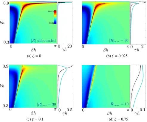
Results are reported in Fig. 10. The dispersion relation in the real problem is visible by means of diverging (in the lossless case) or large (in the lossy case) values of the scattering coefficients when an incident evanescent wave is considered (as in Fig. 9); in Fig. 10, log |Rnum| is reported
in colorscale in the (kh, h) plane, and the red regions reveal the shape of the dispersion relation. The dispersion relation in the homogenized problem, Eq. (50), is also reported (black lines) applying the criterion k < kmp1 ⇠2for an efficient guiding e↵ect. The agreement is good but
remains qualitative since the criterion for the disappearance of guided waves is obviously quite subjective.
To end the comparison, it is worth noting that (Rh,Th) can be calculated from (46) using
the same trick as used to compute (Rnum,Tnum) in the real problem (namely using k cos ✓ ! i
k sin ✓ ! in (46)). We get in the plane (kh, h) the wave properties for propagating waves when <k and guided wave when > k. The results are not reported since they are indiscernible at naked eyes to the result reported in Fig. 10. We get |Rh Rnum|/|Rnum| averaged in the whole plane
of 20% for ⇠ = 0.025, 6% for ⇠ = 0.1, and 3% for ⇠ = 0.75 (the comparison is not possible for ⇠ =0). The increase in the error for small ⇠ is mainly attributable to numerical errors for > k. 4. Concluding remarks and perspectives
We have proposed a homogenization of an array of locally resonant inclusions with high contrast in its shear modulus compared to the matrix; this produces wavelengths inside the soft inclusions of the same order of magnitude as their typical size. Such homogenization leads to
0.9 0.3 kh h 0 0 h20 max min |R| unbounded 2 h 0 0 h |R|max= 90 (a) ⇠ = 0 (b) ⇠ = 0.025 h 0 0.3 0.9 kh 0.5 0 h |R|max= 30 h 0 0 0.1 h |R|max= 10 (c) ⇠ = 0.1 (d) ⇠ = 0.75
Figure 10: For (a-d), the left panel reports the reflection coefficient log |Rnum| (colorscale) in the plane (k, ); the dispersion
relation of the guided wave is visible by means of high values of |Rnum|. The dispersion relation of the guided wave in
the homogenized problem, Eq. (50) are reported in black lines, together with the condition k < kmp1 ⇠ (see the main
text). For (a-d) the right panel shows the real part (solid line) and the imaginary part (dotted line) of as a function of kh; the guiding e↵ect becomes inefficient for i> r.
an equivalent problem in which jump conditions apply across the region originally occupied by the array. The homogenized problem has been validated by comparison with direct numerical calculations, and we addressed the case of lossy inclusions.
There are at least three natural extensions of the present study, being of di↵erent nature. One of them is technically rather incremental. We considered shear waves in a binary structures but the present work can be extended without technical difficulties to three dimensional case and to ternary structure, as proposed in Liu et al. (2000). This extension may be of particular interest when locally resonant materials are considered in the acoustic case; as previously said, this is obtained in practice considering binary or ternary structures mixing fluids and elastic materials, thus for which the conversions between shear and longitudinal waves have to be accounted for. We believe that this is the key point to properly describe the negative index material reported in this context (Ding et al., 2007).
The second extension is not demanding at all theoretically but it deserves interest. As pre-viously said, e↵ective medium theories have been applied to locally resonant materials to get e↵ective mass densities ⇢e↵ and e↵ective shear moduli Ge↵. Although these results hold when
the resonant material occupies a thick slab, it is tempting to see if (i) it is possible to replace 18
our e↵ective jump conditions by the usual continuity relations (of the displacement and of the normal stress) at the boundary of a slab filled with some homogeneous e↵ective medium and (ii) if/when the case, how the resulting e↵ective mass density and shear modulus compare with the values (⇢e↵,Ge↵) previously derived in Auriault and Boutin (2012) and in Felbacq and Bouchitt´e
(2005).
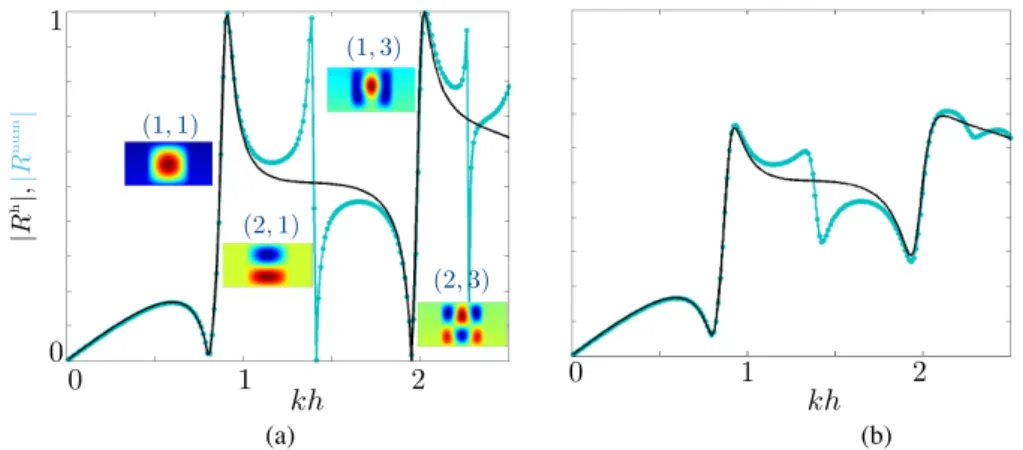
The third extension is technically much demanding. Our result has a serious limitation, in fact the same as in Auriault and Boutin (2012) and Felbacq and Bouchitt´e (2005) (and this was already pointed out in this latter reference). The analysis holds for resonances with non null mean value (namely, n1and n2odd in (5)); this is illustrated in Fig. 11, where the resonances with null
mean value are clearly not described by the homogenized solution. Although these resonances have a higher quality factor and thus are much more sensitive to losses (see Fig. 11(b)), the accuracy of the homogenized solution would be greatly enhanced if one is able to account for them. This requires to develop the homogenization model up to the second order in ⌘ and this is not incremental. For the time being, the model is limited to the first monopolar resonance, and this holds for the homogenization of thick structures.
|R h |, |R n um | 1 0 kh 0 1 2 (1, 1) (2, 1) (2, 3) (1, 3) kh 2 0 1 (a) (b)
Figure 11: Reflection coefficient |Rnum| (symbols) and |Rh| (black lines) as a function of the dimensionless frequency kh
(same representation as in Fig. 6 extended to the first 4 resonances). (a) without attenuation, the four resonances are visible, parametrized by (n1,n2) (the inset shows the corresponding patterns for |X1| < e/2 and X22 [0, 1]), among which
two are of null spatial means: (2,1) and (2,3). (b) same representation for ⇠ = 0.05.
Acknowledgment The authors thank the referees for their useful comments. J.-J.M. thanks the support of the French Agence Nationale de la Recherche (ANR), under grant Aramis (ANR-12-BS01-0021) ”Analysis of Robust Asymptotic Methods In numerical Simulation in mechanics”. Appendix A. Solution of the Dirichlet problem for rectangular inclusions
The solution of (28) is easy to find; introducing U ⌘ Vk 1, U is solution of
in ⌦i 8 >>>< >>>: U + 2U = 2, U|@⌦i=0, (A.1) 19
and U can be expanded onto a basis of eigenfunctions Pn(y) being solutions of the eigenvalue
problem P + 2P = 0 in ⌦
i, with P|@⌦i =0 (we denote nthe eigenvalues). The decomposition
reads
U(y) = UnPn(y). (A.2)
Projecting (A.1) onto the Pngives the coefficients Un
Un= 2
2 2 n
(1, Pn), (A.3)
with (., .) the scalar product. Iny coordinates, our rectangular inclusions have dimensions e/h along y1and ' along y2, and the eigenfunctions are
Pn(y1,y2) = pee2h 2sin n1⇡h e y1 ! sin n2⇡ ' y2 ! ,
with (n1,n2) ordered by n; for instance n = 1 corresponds to n1=n2 =1. We get 8 >>>>> >>< >>>>> >>: 2n= n1⇡h e !2 + n2⇡h 'h !2 , (1, Pn) = 8 ⇡2 r e' h 1 n1n2, (A.4)
for (n1,n2) odd. The interface parameter D in (37) can be calculated
D = ⇢i ⇢m Z ⌦i dy ⇥1 + UnPn(y)⇤ = ⇢i ⇢m " Si 2 2 2 n(1, Pn) 2#, (A.5)
with Si=e'/h and using (A.4), we get
8 >>>>> >>>< >>>>> >>>: D = ⇢i ⇢m e' h " 1 ↵2 n k 2 i k2 i k2i,n # , with k2 i,n⌘ ✓ n1⇡ e ◆2 + n2⇡ h' !2 , and ↵n⌘ 8 ⇡2n1n2, (A.6)
with the ki,nbeing the resonance frequencies in the inclusions, and n = (n1,n2) with n1 and n2
odd integer.
Achaoui, Y., Khelif, A., Benchabane, S., Robert, L., Laude, V., 2011. Experimental observation of locally-resonant and bragg band gaps for surface guided waves in a phononic crystal of pillars. Physical Review B 83 (10), 104201. Auriault, J., 1994. Acoustics of heterogeneous media: macroscopic behavior by homogenization. Curr. Topics Acoust.
Res. I, 63–90.
Auriault, J.-L., Boutin, C., 2012. Long wavelength inner-resonance cut-o↵ frequencies in elastic composite materials. International Journal of Solids and Structures 49 (23), 3269–3281.
Bakhvalov, N. S., Panasenko, G., 1989. Homogenisation: averaging processes in periodic media: mathematical problems in the mechanics of composite materials. Kluver, Dordrecht.
Bonnet-Bendhia, A., Drissi, D., Gmati, N., 2004. Simulation of mu✏er’s transmission losses by a homogenized finite element method. J. Comp. Acoustics 12 (03), 447–474.
Bouchitt´e, G., Bourel, C., Felbacq, D., 2009. Homogenization of the 3d maxwell system near resonances and artificial magnetism. Comptes Rendus Math´ematique 347 (9), 571–576.
Bretagne, A., Tourin, A., Leroy, V., 2011. Enhanced and reduced transmission of acoustic waves with bubble meta-screens. Applied Physics Letters 99 (22), 221906.
Brunet, T., Leng, J., Mondain-Monval, O., 2013. Soft acoustic metamaterials. Science 342 (6156), 323–324.
Campione, S., Lanneb`ere, S., Aradian, A., Albani, M., Capolino, F., 2012. Complex modes and artificial magnetism in three-dimensional periodic arrays of titanium dioxide microspheres at millimeter waves. The Journal of the Optical Society of America B 29 (7), 1697–1706.
Capdeville, Y., Marigo, J.-J., 2013. A non-periodic two scale asymptotic method to take account of rough topographies for 2-d elastic wave propagation. Geophysical Journal International 192 (1), 163–189.
Christensen, J., Romero-Garc´ıa, V., Pic´o, R., Cebrecos, A., de Abajo, F. G., Mortensen, N. A., Willatzen, M., S´anchez-Morcillo, V. J., 2014. Extraordinary absorption of sound in porous lamella-crystals. Scientific reports 4.
Cordero, M.-L., Maurel, A., Mercier, J.-F., Felix, S., Barra, F., 2015. Tuning the wavelength of spoof plasmons by adjusting the impedance contrast in an array of penetrable inclusions. Applied Physics Letters 107 (8), 084104. David, M., Marigo, J.-J., Pideri, C., 2012. Homogenized interface model describing inhomogeneities located on a surface.
Journal of Elasticity 109 (2), 153–187.
Delourme, B., 2015. High-order asymptotics for the electromagnetic scattering by thin periodic layers. Mathematical Methods in the Applied Sciences 38 (5), 811–833.
Delourme, B., Haddar, H., Joly, P., 2012. Approximate models for wave propagation across thin periodic interfaces. Journal de math´ematiques pures et appliqu´ees 98 (1), 28–71.
Ding, Y., Liu, Z., Qiu, C., Shi, J., 2007. Metamaterial with simultaneously negative bulk modulus and mass density. Physical Review Letters 99 (9), 093904.
Elford, D. P., Chalmers, L., Kusmartsev, F., Swallowe, G., 2010. Acoustic band gap formation in metamaterials. Interna-tional Journal of Modern Physics B 24 (25n26), 4935–4945.
Felbacq, D., 2015. Impedance operator description of a metasurface with electric and magnetic dipoles. Mathematical Problems in Engineering 2015.
Felbacq, D., Bouchitt´e, G., 2005. Theory of mesoscopic magnetism in photonic crystals. Physical Review Letters 94 (18), 183902.
Go↵aux, C., S´anchez-Dehesa, J., Lambin, P., 2004. Comparison of the sound attenuation efficiency of locally resonant materials and elastic band-gap structures. Physical Review B 70 (18), 184302.
Go↵aux, C., S´anchez-Dehesa, J., Yeyati, A. L., Lambin, P., Khelif, A., Vasseur, J., Djafari-Rouhani, B., 2002. Evidence of fano-like interference phenomena in locally resonant materials. Physical Review Letters 88 (22), 225502. Guenneau, S., Movchan, A., P´etursson, G., Ramakrishna, S. A., 2007. Acoustic metamaterials for sound focusing and
confinement. New Journal of physics 9 (11), 399.
Ho, K. M., Cheng, C. K., Yang, Z., Zhang, X., Sheng, P., 2003. Broadband locally resonant sonic shields. Applied physics letters 83 (26), 5566–5568.
Jin, Y., Fernez, N., Pennec, Y., Bonello, B., Moiseyenko, R. P., H´emon, S., Pan, Y., Djafari-Rouhani, B., 2016. Tunable waveguide and cavity in a phononic crystal plate by controlling whispering-gallery modes in hollow pillars. Physical Review B 93 (5), 054109.
Lai, Y., Wu, Y., Sheng, P., Zhang, Z.-Q., 2011. Hybrid elastic solids. Nature materials 10 (8), 620–624.
Lanneb`ere, S., Campione, S., Aradian, A., Albani, M., Capolino, F., 2014. Artificial magnetism at terahertz frequencies from three-dimensional lattices of tio 2 microspheres accounting for spatial dispersion and magnetoelectric coupling. The Journal of the Optical Society of America B 31 (5), 1078–1086.
Lapine, M., McPhedran, R., Poulton, C., 2016. Slow convergence to e↵ective medium in finite discrete metamaterials. Physical Review B 93 (23), 235156.
Liu, Z., Zhang, X., Mao, Y., Zhu, Y., Yang, Z., Chan, C., Sheng, P., 2000. Locally resonant sonic materials. Science 289 (5485), 1734–1736.
Lombard, B., Maurel, A., Marigo, J.-J., 2016. Numerical modeling of the acoustic wave propagation across an homoge-nized rigid microstructure in the time domain. arXiv preprint arXiv:1607.08836.
Marigo, J.-J., Maurel, A., 2016a. Homogenization models for thin rigid structured surfaces and films. The Journal of the Acoustical Society of America 140 (1), 260–273.
Marigo, J.-J., Maurel, A., 2016b. An interface model for homogenization of acoustic metafilms. to appear.
Marigo, J.-J., Maurel, A., 2016c. Two-scale homogenization to determine e↵ective parameters of thin metallic-structured films. In: Proc. R. Soc. A. Vol. 472. The Royal Society, p. 20160068.
Marigo, J.-J., Maurel, A., Pham, K., Sbitti, A., 2016. E↵ective dynamic properties of a row of elastic inclusions. submit-ted.
Marigo, J.-J., Pideri, C., 2011. The e↵ective behavior of elastic bodies containing microcracks or microholes localized on a surface. International Journal of Damage Mechanics, 1056789511406914.
Maurel, A., Marigo, J.-J., Ourir, A., 2016. Homogenization of ultrathin metallo-dielectric structures leading to transmis-sion conditions at an equivalent interface. The Journal of the Optical Society of America B 33 (5), 947–956. Maurel, A., Mercier, J.-F., F´elix, S., 2014. Wave propagation through penetrable scatterers in a waveguide and through a
penetrable grating. The Journal of the Acoustical Society of America 135 (1), 165–174.
Mercier, J.-F., Cordero, M.-L., F´elix, S., Ourir, A., Maurel, A., 2015. Classical homogenization to analyse the dispersion 21
relations of spoof plasmons with geometrical and compositional e↵ects. Proc. R. Soc. A 471, 20150472.
O’Brien, S., Pendry, J. B., 2002. Photonic band-gap e↵ects and magnetic activity in dielectric composites. Journal of Physics: Condensed Matter 14 (15), 4035.
Pham, K., Kouznetsova, V. G., Geers, M. G., 2013. Transient computational homogenization for heterogeneous materials under dynamic excitation. Journal of the Mechanics and Physics of Solids 61 (11), 2125–2146.
Sanchez-Palencia, E., 1987. Elastic body with defects distributed near a surface. In: Homogenization Techniques for Composite Media. Springer, pp. 183–192.
Zhao, H., Wen, J., Yu, D., Wen, X., 2010. Low-frequency acoustic absorption of localized resonances: Experiment and theory. Journal of Applied Physics 107 (2), 023519.
Zhikov, V., 2005. On spectrum gaps of some divergent elliptic operators with periodic coefficients. ST PETERSBURG MATHEMATICAL JOURNAL C/C OF ALGEBRA I ANALIZ 16 (5), 773.
Zhikov, V. V., 2000. On an extension of the method of two-scale convergence and its applications. Sbornik: Mathematics 191 (7), 973.