Implementation trade-offs for FGPA accelerators

HAL Id: tel-01755720

https://tel.archives-ouvertes.fr/tel-01755720

HAL is a multi-disciplinary open access archive for the deposit and dissemination of sci-entific research documents, whether they are pub-lished or not. The documents may come from teaching and research institutions in France or abroad, or from public or private research centers.

L’archive ouverte pluridisciplinaire HAL, est destinée au dépôt et à la diffusion de documents scientifiques de niveau recherche, publiés ou non, émanant des établissements d’enseignement et de recherche français ou étrangers, des laboratoires publics ou privés.

Implementation trade-offs for FGPA accelerators

Gaël Deest

To cite this version:

Gaël Deest. Implementation trade-offs for FGPA accelerators. Computer Arithmetic. Université Rennes 1, 2017. English. �NNT : 2017REN1S102�. �tel-01755720�

ANNÉE 2017

THÈSE / UNIVERSITÉ DE RENNES 1

sous le sceau de l’Université Bretagne Loire

pour le grade de

DOCTEUR DE L’UNIVERSITÉ DE RENNES 1

Mention : Informatique

Ecole doctorale MathSTIC

présentée par

Gaël Deest

préparée à l’unité de recherche 6074 - IRISA

Institut de recherche en informatique et systèmes Aléatoires

UFR Informatique Électronique

Implementation

Trade-Offs for FPGA

Accelerators

Thèse soutenue à Rennes le 14 décembre 2017 devant le jury composé de :

Albert COHEN

DR Inria Rocquencourt / rapporteur

Florent DE DINECHIN

PR INSA Lyon / rapporteur

Karine HEYDEMANN

MCF Université Pierre et Marie Curie / examinatrice

Daniel MÉNARD

PR INSA Rennes / examinateur

Tomofumi YUKI

CR Inria Rennes / examinateur

Steven DERRIEN

Remerciements

Chaque thèse est une expérience unique. Si, pour certains, il semble ne s’agir que d’un rite de passage sans réelle difficulté, tel ne fut assurément pas mon cas. Au cours

de ces✘✘

✘

trois quatre années éprouvantes, ponctuées de doutes et de joies, d’intuitions et d’espoirs déçus, j’ai eu la chance d’être entouré de gens formidables, sans l’appui desquels ce manuscrit n’existerait sans doute pas.

En premier lieu, je remercie mes directeurs de thèse, Steven Derrien et Olivier Sentieys, d’avoir accordé leur confiance au vieil étudiant que j’étais et de m’avoir ouvert les portes de l’équipe Cairn, d’abord comme stagiaire, puis comme doctorant. En outre et en particulier, je remercie Steven pour sa tutelle scientifique exigeante, parfois dure mais souvent juste – si j’ai un tant soit peu appris à ravaler mon orgueil, me poser les bonnes questions et raisonner en chercheur, c’est en grande partie grâce à lui.

On ne saurait trop souligner l’apport de Tomofumi Yuki à ces travaux. Si, décidé-ment, mon esprit trop français a bien du mal à appréhender le concept de punchline, son attachement à me l’expliquer encore et encore illustre bien sa considérable pa-tience. Je le remercie encore pour sa rigueur, sa bienveillance et son humilité.

Je remercie le jury d’avoir accepté la charge d’évaluer ces travaux. La pertinence de leurs remarques et questions prouve qu’ils se sont acquittés de cette tâche avec un sérieux remarquable – j’en suis profondément honoré. En particulier, j’adresse de profonds remerciements à mes deux rapporteurs, Albert Cohen et Florent de Dinechin, pour la lecture approfondie qu’ils ont faite de ce manuscrit et leur regard expert sur mes contributions.

Je remercie tous les membres de l’équipe Cairn, permanents, post-docs, doctor-ants et stagiaires, présents et passés, de m’avoir si bien accueilli parmi eux. Que serait une journée au labo sans les deux pauses réglementaires et les débats plus ou moins trollesques qui les animent ? En vrac, et de façon non exhaustive, je re-mercie chaleureusement Ali Hassan El Moussawi, Antoine Morvan, Nicolas Simon, Christophe Huriaux, Laurent Perraudeau, Angeliki Kritikakou, Patrice Quinton, Nicolas Estibals, Baptiste Roux, Simon Rokicki, Thomas Levesque, Rafail Psiakis. . .

Merci à notre assistante, Nadia Derouault, pour sa gentillesse, son humanité, sa prévenance et son indulgence quant à ma totale incompétence administrative.

Merci aussi à mes anciens comparses de Master rennais, devenus de précieux amis, tant pour les discussions enflammées sur IRC que leur soutien moral: Simon Bouget, Gabriel Radanne, Benoit Le Gouis et Nicolas Braud-Santoni.

Je remercie également mon ami de quinze ans, Jérémy Hervé, tant pour son affection et son humour décapant que pour avoir été là dans les moments difficiles. Sans doute ignorais-tu, en me parlant de FPGA en 2002, que je finirais par faire une

thèse sur le sujet, après un chemin bien sinueux !

Merci à ma famille pour tout ce qu’elle m’a enseigné, malgré les épreuves et les tempêtes.

Merci enfin à celle dont je partage la vie depuis plus de onze années et qui a cru en moi comme personne, vivant ces dernières années avec la même intensité que moi: Caroline, mon Amour.

Contents

0.1 Contexte . . . 13

0.2 Compromis entre coût et précision . . . 14

0.3 Compromis pour l’implémentation de stencils . . . 16

0.4 Perspectives . . . 17 0.5 Conclusion . . . 17 1 Introduction 19 1.1 Context . . . 19 1.2 Hardware Accelerators . . . 20 1.3 Accelerator Design . . . 21

1.4 Presentation of This Work . . . 22

2 Accuracy Evaluation 23 2.1 Introduction . . . 23

2.2 Hardware Representation of Real Numbers . . . 24

2.2.1 Fixed-Point Arithmetic . . . 24

2.2.2 Floating-Point Arithmetic . . . 25

2.2.3 Comparison . . . 27

2.2.4 Summary . . . 29

2.3 Floating-Point to Fixed-Point Conversion . . . 29

2.3.1 Problem Setup . . . 29

2.3.2 Range Estimation . . . 31

2.3.3 Accuracy Metrics . . . 31

2.3.4 Accuracy Evaluation . . . 33

2.4 Analytical Accuracy Evaluation . . . 33

2.4.1 Signal-Flow Graphs . . . 34

2.4.2 Error Sources . . . 35

2.4.3 Pseudo Quantization Noise model . . . 36

2.4.4 Operator-Level Noise Propagation . . . 37

2.4.5 Noise Propagation in Linear Systems . . . 38

2.4.6 Noise Propagation in Non-Linear Systems . . . 40

2.4.7 System-Level Approaches . . . 40

2.5 Limitations of Analytical Accuracy Evaluation . . . 41

3 Improving Applicability of Source-Level Accuracy Evaluation 43 3.1 Introduction . . . 43

3.3 Linear Shift-Invariant Systems . . . 45

3.3.1 Signals . . . 45

3.3.2 Linear Shift-Invariant Systems . . . 46

3.3.3 Algebraic Structure of LSI Systems . . . 47

3.3.4 Impulse Response . . . 48

3.3.5 Transfer Function and Z-Transform . . . 48

3.3.6 Frequency Response . . . 50

3.4 Analytical Accuracy Evaluation for LSI Systems . . . 50

3.4.1 Overview . . . 50

3.4.2 Multidimensional Flow-Graphs . . . 51

3.4.3 Inference of MDFGs from Source Code . . . 52

3.4.4 Computation of Transfer Functions . . . 58

3.4.5 Quantization of Coefficients . . . 58

3.4.6 Accuracy Model Construction . . . 60

3.5 Experimental Validation . . . 62

3.6 Future Work and Extensions . . . 63

3.7 Conclusion . . . 64

4 Implementation and Optimization of Stencil Computations 65 4.1 Introduction . . . 65 4.2 Definitions . . . 66 4.2.1 Classification . . . 66 4.2.2 Boundary Conditions . . . 66 4.3 Examples . . . 67 4.3.1 Cellular Automata . . . 67 4.3.2 Smith-Waterman . . . 68 4.3.3 Finite-Difference Methods . . . 68 4.4 Implementation Challenges . . . 71 4.5 Tiling Transformation . . . 72

4.5.1 Iteration Space and Dependences . . . 73

4.5.2 Schedule . . . 73

4.5.3 Dependence Relation . . . 74

4.5.4 Tiling . . . 75

4.5.5 Tile-Level Dependencies . . . 76

4.5.6 Skewing . . . 77

4.5.7 Tile Halo and Communication Volume . . . 78

4.5.8 Wavefront Parallelism . . . 80 4.5.9 Hierarchical Tiling . . . 81 4.6 Tiling Variants . . . 81 4.6.1 Overlapped Tiling . . . 82 4.6.2 Diamond Tiling . . . 82 4.6.3 Hexagonal Tiling . . . 84 4.7 Memory Allocation . . . 86

4.8 Tile Size Selection . . . 88

5 Managing Trade-Offs in FPGA Implementations of Stencil

Com-putations 91

5.1 Introduction . . . 91

5.2 Architectural Design Space . . . 92

5.2.1 Target Platform . . . 92

5.2.2 Accelerator Overview . . . 92

5.2.3 Compute Actor . . . 93

5.2.4 Overview of the Read/Write Actors . . . 94

5.2.5 Design Parameters . . . 94

5.3 Performance Modeling . . . 96

5.3.1 Asymptotic Performance Model . . . 96

5.3.2 Modeling the Area Cost . . . 97

5.4 Data Layout . . . 98

5.4.1 Example: 3D Iteration Space . . . 99

5.4.2 Generalization . . . 100

5.5 Implementation . . . 100

5.5.1 Code Generator Overview . . . 101

5.5.2 HLS Code Overview . . . 101 5.6 Experimental Validation . . . 104 5.6.1 Experimental Setup . . . 104 5.6.2 Full Tiling . . . 106 5.6.3 Partial Tiling . . . 108 5.7 Discussion . . . 109

5.7.1 Comparison with Earlier Work . . . 109

5.7.2 Additional Considerations . . . 110

5.8 Conclusions . . . 111

6 Conclusion 113 6.1 Review of our Contributions . . . 113

6.2 Perspectives . . . 115

List of Figures

2.1 Qm,n format with m-bit integral part and n-bit fractional part. . . 24

2.2 Fixed-point addition of two 5-bit numbers. . . 25

2.3 Binary Representation of a IEEE 754 Floating-Point Number . . . 26

2.4 Maximum representation error of floating-point numbers as a function of represented value. . . 28

2.5 Dynamic range of floating-point and fixed-point representation. . . . 29

2.6 PDF of the sum of 5 i.i.d random variables with distribution U([0, 1]). 32 2.7 SFG of a FIR Filter computing the formula: y(n) = �3 i=0bix(n − i). Nodes labeled z−1 _{represent one-cycle delays and triangle-shaped} nodes multiplication by a constant coefficient. . . 34

2.8 FIR filter implementation for the Id.Fix conversion tool. . . 35

2.9 Introduction of error sources in a Signal Flow Graph. . . 36

2.10 PQN characteristics based on input / output signal precision and quantization mode. q represents the quantization step and k the number of eliminated bits when converting between fixed-point for-mats. Note that when k → ∞, the discrete model converges towards the continuous model. . . 37

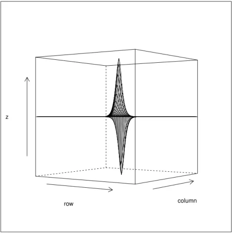
3.1 Impulse Response of the deriche edge detector estimated by our tool (horizontal gradient). . . 49

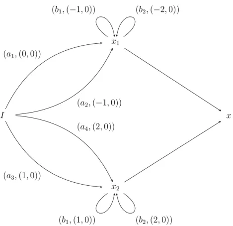
3.2 Relation between the impulse response, transfer function and fre-quency response of a system T . The transfer function Hz,T is the Z-transform of the impulse response. The frequency response HT is obtained by restricting the transfer function to the unit circle for each component. Finally, hT and HT are related by the Fourier transform. 51 3.3 Partial flowgraph of the Deriche filter . . . 52

4.1 1D Jacobi stencil. . . 65

4.2 Glider pattern in Game of Life. . . 67

4.3 Seismic Modeling. . . 70

4.4 Roofline Model . . . 72

4.5 Naive Gauss-Seidel stencil implementation . . . 73

4.6 . . . 74

4.7 Tiling of a 1D Gauss-Seidel stencil with 2 × 2 rectangular tiles. . . 76

4.8 Tiled source code of the 1D Gauss-Seidel stencil. . . 77

4.9 Invalid tiling for a Jacobi skewing. . . 78

4.11 Tile wavefronts for the 1D Gauss-Seidel stencil. . . 80 4.12 Wavefront parallelism extraction as an application of skewing

(Gauss-Seidel stencil). . . 81 4.13 Overlapped tiling . . . 83 4.14 Shape of minimal tile halo for overlapped tiling . . . 83 4.15 Diamond tiling for 1D 3-point Jacobi stencil. Tiling hyperplanes

(dashed lines) are inferred from faces of the dependence cone, spanned by dependence vectors (red arrows). Each horizontal band of tiles can benefit from concurrent start. Note the heterogeneous shape of tiles in consecutive bands. . . 84 4.16 Illustration of hexagonal tiling, a generalization of diamond tiling.

Unlike diamond tiling, the elongated top and bottom faces guarantee a minimum amount of intra-tile parallelism at each time step, while still

allowing concurrent start along one of the iteration space boundaries. 85

4.17 Similarly to hexagonal tiling, split tiling improves upon diamond tiling by enabling concurrent start while preserving fine-grained parallelism. 86 5.1 Diagram of the architecture. . . 93 5.2 Illustration of partial tiling for a 2D jacobi. . . 95 5.3 Input faces of a tile. . . 99 5.4 Use of the DATAFLOW directive to implement computation /

commu-nication overlapping. . . 102 5.5 Predicted and measured area/throughput for the Jacobi2D kernel. . . 105 5.6 Predicted and measured area/throughput for the Anisotropic

Diffu-sion kernel. . . 106 5.7 Area results of partial tiling for the two kernels and different

List of Tables

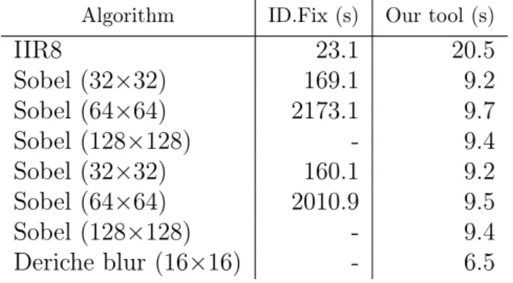
2.1 Interpretation of a IEEE 754 Floating-Point Number . . . 26 3.1 Model construction time for our tool and ID.Fix. . . 62 3.2 Validation of our model against simulations and ID.Fix. . . 63 5.1 Number of floating-point operations, and pipeline depth for one

up-date of the kernels. . . 104 5.2 Resource Usage for the Jacobi 2D kernel . . . 107 5.3 Resource Usage for the Anisotropic Diffusion kernel . . . 108

Résumé en français

0.1

Contexte

Des téléphones aux centres de calcul, les systèmes informatiques jouent aujourd’hui un rôle majeur dans la plupart des activités humaines. On les retrouve dans des contextes variés, dont la diversité reflète celle de leurs applications. En première approche, on peut distinguer trois types de système informatique:

Les systèmes généralistes, comme les stations de travail, sont conçus pour effectuer raisonnablement efficacement un bon nombre de tâches (comme naviguer sur le web, utiliser une suite bureautique ou jouer à des jeux vidéos). Leur principale caractéristique est leur flexibilité, puisqu’ils peuvent exécuter des programmes arbitraires installés ou écrits par l’utilisateur final.

Les systèmes embarqués, en revanche, sont spécifiquement dédiés à une ou quelques tâches bien spécifiques. Ils sont enfouis dans toutes sortes de système, des smartphones (où ils accélèrent par exemple les opérations d’encodage/décodage) au module de commande des engins spatiaux. Ils se caractérisent par les con-traintes fortes qui pèsent sur leur conception. En effet, ils doivent par exemple respecter des contraintes de latence (temps réel), de consommation énergé-tique, de taille, de coût et de tolérance aux fautes – souvent simultanément. Les super-ordinateurs, par contraste, sont optimisés pour des tâches de calcul

in-tensif, comme les simulations scientifiques (par exemple en climatologie ou météorologie) et l’intelligence artificielle (réseaux de neurones). Par rapport aux systèmes généralistes, la différence majeure est leur grande puissance de calcul, puisqu’ils doivent effectuer un grand nombre d’opérations par seconde pour satisfaire aux exigences de performance.

Toutes ces différences influent sur la façon dont ces systèmes sont conçus et pro-grammés. Par exemple, afin de supporter un grand nombre de cas d’utilisation, les ordinateurs généralistes sont basés sur des processeurs génériques offrant un jeu d’instruction prédéfini. Afin d’améliorer les performances, plusieurs straté-gies sont mises en oeuvre dans ces architectures, comme l’utilisation de plusieurs niveaux de cache ou de techniques superscalaires. Ainsi, un processeur moderne peut, par exemple, ordonner les instructions dynamiquement en fonction des ressources disponibles, ou “deviner” la valeur d’une condition de branchement à partir du passé afin d’exécuter certaines parties du code par avance. Ces mécanismes complexes profitent à la fois aux programmeurs et aux utilisateurs finaux:

• Le même jeu d’instruction peut être réutilisé d’une génération de processeur à l’autre, fournissant une inter-compatibilité ascendante et descendante entre logiciel et matériel.

• Les programmes peuvent être écrits dans un langage de programmation haut niveau, traduit ensuite en une série d’instruction élémentaires par un compi-lateur, sans qu’il soit nécessaire de connaître précisément l’architecture sous-jacente.

• Les techniques d’optimisation statiques (à la compilation) et dynamiques (mises en oeuvre lors de l’exécution, comme les techniques superscalaires) assurent dans la plupart des cas des performances décentes aux utilisateurs, sans efforts excessifs de la part des programmeurs.

Ces commodités ont rendu possible les environnements logiciels sophisitiqués que nous utilisons quotidiennement. Malheureusement, ces avantages ne sont pas gratu-its: par nature, les architectures génériques ne peuvent fournir des performances ou une efficacité optimales, quelle que soit l’application.

En fait, les processeurs génériques représentent un compromis pertinent entre performance et flexibilité. Si ce compromis convient à beaucoup d’applications, tel n’est pas toujours le cas. Par exemple, dans le cadre de systèmes embarqués haute-ment contraints en ressources, l’utilisation de processeurs génériques peut entraîner un dépassement du budget alloué en termes de surface de silicium ou de consom-mation énergétique. L’utilisation d’architectures spécifiques, nommées accélérateurs matériel, s’impose alors.

Cette thèse traite la conception de tels d’accélérateurs (plus spécifiquement d’accélerateurs implémentés sur FPGA). Nous nous intéressons à la conception de modèles de performance permettant la mise en oeuvre de compromis spécifiques à chaque application, selon diverses métriques (précision, surface, débit, etc.). Ce manuscrit est composé de deux parties majeures: dans les chapitres 2 et 3, l’on s’intéresse aux compromis entre précision et coût matériel (notamment). Dans les chapitres 4 et 5, on se concentre sur une classe d’applications, les stencils. Le reste de ce chapitre présente succintement ces deux problématiques et nos contributions.

0.2

Compromis entre coût et précision

Dans la première moitié de ce manuscrit, on s’intéresse à la précision des résultats. Les compromis portant sur la précision représentent un vaste champ d’opportunités pour les architectes matériel. Un exemple classique est l’utilisation de l’arithmétique en virgule fixe au lieu de l’arithmétique en virgule flottante pour réduire les coûts matériel et la consommation énergétique. Naturellement, la précision ne peut être réduite indéfiniment: chaque implémentation doit satisfaire à des contraintes de précision spécifiques, dont le respect doit être vérifié lors de l’exploration de l’espace de conception.

Déterminer si une implémentation en virgule fixe donnée respecte une contrainte de précision représente un problème difficile en général. On peut distinguer deux classes de techniques: simulatoires et analytiques. Les techniques basées sur la

simulation sont facilement applicables et offrent de bons résultats à condition de disposer de suffisamment d’échantillons. Cependant, elles sont lentes à mettre en oeuvre car estimer la précision de chaque solution requiert un grand nombre d’exécutions. Les modèles analytiques sont beaucoup plus rapides à évaluer, ce qui permet l’exploration de plus de solutions en peu de temps, et donc l’identification de meilleur compromis. Cependant, leur applicabilité limitée représente un défi majeur. Avant ces travaux, les techniques analytiques ne pouvaient traiter que des sys-tèmes uni-dimensionnels. dans le chapitre 3, nous étendons les techniques précé-dentes à des algorithmes multi-dimensionnels, comme des filtres d’image. Nous nous concentrons sur les filtres Linéaires, Spatialement Invariants (LSI), une généralisa-tion des filtres Linéaires, Invariants dans le Temps supportés par d’autres approches. Nous proposons un flot partant d’une description algorithmique (écrite en C/C++). Les deux principaux défis que nous relevons sont:

• Extraire une représentation mathématique compacte d’un filtre linéaire à partir d’une description impérative en C/C++.

• Dériver un modèle de précision fiable à partir d’une telle représentation. Le premier de ces défis est relevé dans le cadre du modèle polyédrique. Nous représentons les filtres LSI comme des Systèmes d’Équations aux Récurrences Uni-formes (SUREs) ou, de façon équivalente, des graphes de flots de donnée multi-dimensionnels (MDFGs), par analogie aux graphes de flot de signal (SFGs) utilisés comme représentation intermédiaire par les approches précedentes.

Une différence majeure entre SFGs et MDFGs est que les MDFGs / SUREs n’imposent pas d’ordre d’itération canonique à chaque dimension. Cela nous per-met de supporter des filtres d’image récursifs complexes, scannant leurs entrées dans toutes les directions. Nous utilisons des techniques polyédriques d’analyse de dépen-dance afin de transformer le programme en systèmes d’équation aux récurrences affines. Un certain nombre de simplifications et de transformations sont requises, comme l’uniformisation des dépendances, avant que le système puisse être reconnu comme un SURE.

Pour la seconde problématique – inférer des modèles de précision – nous pro-posons deux approches. Toutes deux se ramènent à calculer l’intégrale et la norme

L2 _{de la réponse impulsionnelle du filtres, mais depuis des points de vue duaux:}

• Dans le domaine temporel, nous dérivions ces sommes en déroulant / évaluant les équations de récurrence définissant le système.

• Dans le domaine fréquentiel, nous exploitons les propriétés algébriques des fonctions de transfert pour calculer celles représentant la propagation de chaque erreur. Nous calculons alors les sommes requises à partir de la réponse fréquen-tielle.

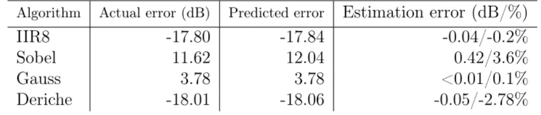
Pour le deuxième cas, nous proposons une version simplifiée et plus efficace de l’algorithme proposé par Ménard et al. [23]. Nos expériences démontrent que nos modèles sont obtenus rapidement, et leur efficacité est illustrée en comparant avec des simulations sur des données réelles.

Finalement, nous montrons comment l’approche fréquentielle peut être utilisée en amont de l’optimisation des largeurs afin de traiter la quantification des coefficients, un problème généralement ignoré dans les autres travaux.

0.3

Compromis pour l’implémentation de stencils

Dans la seconde partie de cette thèse, nous nous concentrons sur les compromis possibles pour l’implémentation de stencils itératifs sur FPGA. Les stencils itératifs (ou plus simplement stencils) sont un motif de calcul retrouvé dans de nombreuses applications, des simulations scientifiques à la vision par ordinateur. Chaque appli-cation présente des contraintes spécifiques en fonction de la taille du domaine, du schéma de dépendance et des caractéristiques intrinsèques du calcul.

En première approche, les performances d’un stencil sont principalement déter-minées par les ressources de calcul utilisées et les performances de la mémoire. Le pavage (ou tiling), présenté dans le chapitre 4, est un outil essentiel pour optimiser ces deux aspects, en améliorant la localité mémoire d’une part et en autorisant la parallélisation à différentes niveaux d’autre part.

Au chapitre 5, nous proposons une méthode systématique pour l’impl’ementation de stencil itératifs sur FPGA. Notre méthode s’appuie sur un gabarit d’architecture flexible, fondé sur le pavage et exposant diverses paramètres:

• Les performances maximales peuvent être controlées en ajustant le facteur de déroulage du chemin de données. Ceci autorise des compromis entre débit et surface.

• Des tuiles plus grandes peuvent être utilisées pour réduire les besoins en bande passante, au prix d’une plus grande utilisastion en mémoire locale.

• L’espace d’itération peut être pavé selon un sous-ensemble de ses dimensions, afin de réduire encore plus l’utilisation en bande passante. Le prix à payer est une perte de contrôle partielle sur l’utilisation en mémoire locale, qui devient proportionnelle à la taille de chaque dimension non pavée.

En outre, nous proposons des modèles de performance simples, dérivés d’une analyse à haut niveau des performances du système. Ces modèles peuvent servir de base à l’exploration de l’espace des solutions.

Pour valider notre architecture et nos modèles, nous avons implémentńotre ap-proche sous la forme d’un outil de génération de code visant Vivado SDSoC. Nous avons identifié, pour différentes cibles de performance, plusieurs solutions poten-tielles en utilisant nos modèles de performance / surface. Nos expériences démon-trent la bonne précision de nos modèles de performance. Nos modèles de surface s’avèrent, bien que moins précis, suffisants pour estimer a priori les solutions les plus intéressantes. Ces modèles ont donc fait la preuve de leur utilité lors de la phase de conception.

Finalement, au cours de ce travail, nous avons constaté l’importance de la conti-guité en mémoire pour réduire la latence et bénéficier des accès bursts proposés par le bus. Nous avons donc conçu une disposition mémoire spécifique pour les tencils.

Pour l’instant, ce layout n’est implémenté que pour les stencils 2D. Sa généralisation à des stencils de dimension supérieure mériterait d’autres travaux.

0.4

Perspectives

Nos travaux ouvrent plusieurs perspectives.

Une direction de recherche évidente consisterait à étendre notre travail sur les modèles de précision à une classe plus grande de programmes, comme les filtres linéaires non-invariants, ou des filtres constitués d’opérations arbitraires. Une autre piste, peut-être plus intéressante, serait de supporter des programmes non polyé-driques. Par exemple, certains algorithmes, comme la transformée de Fourier rapide, présentent de grandes régularités et un flot de contrôle statique sans pour autant être représentables avec des dépendances affines. La propagation des erreurs dans de tels algorithmes présente encore des défis, et nous ne savons pas si le déroulage peut être évité.

On pourrait aussi imaginer utiliser des modèles de précision analytiques dans d’autres contextes, par exemple pour analyser les erreurs de quantification dans des programmes en virgule flottante, ou pour prédire l’impact d’erreurs transitoires (“soft errors”) ou d’opérateurs approximatifs sur la correction du programme. Une difficulté majeure est que, dans de tels cas, les erreurs ne vérifient pas les mêmes propriétés statistiques que le bruit de quantification de le cas de la virgule fixe.

Nos travaux sur les stencils s’appuie sur une compréhension claire des facteurs majeurs affectant leur performance. Des observations similaires peuvent être for-mul’ees pour de nombreux algorithmes. Une approche plus générique, ciblant tous les algorithmes se prêtant au pavage, pourrait probablement être proposée.

Nos recherches sur le placement contigu des données en mémoire. Cette problé-matique, importante en pratique, n’a pas été très étudiée. Elle ouvre des questions intéressantes, comme sur la façon de réduire le nombre de tampons requis ou la né-cessité d’utiliser des mémoires locales pour réordonner les entrées. Nous suspectons l’existence de compromis intéressants entre la séquentialité des données d’une part et leur contiguïté d’autre part. Cependant, cette question mériterait de plus amples investigations.

Pour finir, l’interaction entre les stencils et la précision est difficile à étudier. La capacité des FPGAs à gérer des données de taille arbitraire constitue l’un de leurs avantages majeurs, autorisant des réductions en surface significatives pour les applications supportant une certaine dégradation de la précision. Pouvoir carac-tériser l’impact (par exemple) de formats en virgule fixe sur la précision de stencils autoriserait des compromis très intéressants.

0.5

Conclusion

Lors de la conception d’accélerateurs matériel, le défi majeur réside dans la taille de l’espace de conception à explorer, en particulier quand certaines dimensions de design comme la précision, sont envisagées. Comme chaque application possède des exigences spécifiques, une solution unique ne peut répondre à tous les besoins. Dans

cette thèse, nous défendons une approche rigoureuse de la conception matérielle, basée sur l’utilisation de modèles. Nous avons démontré l’efficacité de cette stratégie à deux problématiques distinctes: les stencils et l’optimisation des largeurs. À mesure que les accélérateurs se répandent, l’utilisation de modèles spécifiques devien-dra essentiel pour comprendre l’impact des choix de conception sur le comportemet du système. Notre travail représente une étape dans cette direction.

Chapter 1

Introduction

1.1

Context

From smartphones to data centers, computer systems now play a major role in most human activities. They are found in vastly different contexts, reflecting the diversity of their applications. We distinguish three main types of computing environments:

General-purpose computers, such as desktop workstations, are designed to run reasonably efficiently a number of applications (e.g., web browsers, office suites or video games). Their main feature is their flexibility, as they can run arbi-trary programs installed or written by the end user.

Embedded systems, on the other hand, are dedicated to some specific task or set of tasks. They can be found within all sorts of systems and devices, from smartphones (where they typically handle encoding/decoding tasks) to the command system of spacecrafts. Their characteristic is the highly constrained environment in which they operate, as they are usually subject to real-time, power, size, cost or fault-tolerance constraints (often at the same time). Supercomputers are optimized towards High-Performance Computing (HPC)

workloads, such as scientific simulations (e.g., climatology, seismology) or chine learning applications. Compared to general-purpose computers, the ma-jor difference is their significant computing power, as they must perform a large number of operations per second to meet performance requirements. All these differences influence the way these systems are designed and pro-grammed. For example, since they must support a large number of use cases, general-purpose computers are based on generic processor design offering a pre-defined instruction set. Several design strategies are used to improve performance, such as adding multiple levels of cache or applying superscalar techniques in the processor. A modern processor may thus, for instance, schedule instructions dy-namically based on available resources, or “guess” the value of a branching condition based on past executions. These complex mechanisms benefits both end users and programmers, since:

• The same instruction set may be used over several CPU generations, providing backward and forward compatibility between software and hardware.

• Compilers can translate programs written in a high-level programming lan-guage into sequences of elementary instructions, without exact knowledge of the supporting architecture.

• Compile- and run-time optimizations (from memory hierarchy to superscalar techniques) ensure that users get decent performance in most cases without excessive optimization efforts from the programmer.

These facilities have made possible the sophisticated software environments that we use daily. Unfortunately, these advantages come at a price: generic architectures cannot, by their very nature, provide optimal performance or efficiency for any particular application.

Generic processors represent a convenient trade-off between performance and flexibility. While this is suitable for many applications, such is not always the case. For instance, in resource-constrained embedded systems, generic processors may exceed power and area budget for a given performance goal. The use of more efficient, special-purpose hardware accelerators is then necessary. Such accelerators, and the the problem of their design, are at the core of this thesis.

1.2

Hardware Accelerators

In a broad sense, the term accelerator denotes any processing device that gives up some genericity to execute a type of computation more efficiently than a general-purpose processor (along which they are commonly used). Floating-point

coproces-sors, such as Intel’s C8087 (introduced in 1980) constitute good examples1

. More generally, for the purpose of this discussion, we distinguish:

• Programmable accelerators, designed for a class of applications while retaining some level of programmability. Well-known examples include Digital Signal Processors (DSPs) and Graphics Processing Units (GPUs). DSPs are special-purpose processors that offer efficient support for common signal processing operations (e.g., dot products). GPUs, on the other hand, have evolved from domain-specific chips into powerful semi-generic computing platforms for data-parallel floating-point computations.

• Custom, fixed-function accelerators, on the other hand, are specifically de-signed for a single, well-defined task. They may be implemented as costly Application-Specific Integrated Circuits (ASICs), or on top of reconfigurable logic, such as Field-Programmable Gate Arrays (FPGAs).

Naturally, fixed-function implementations represent the highest level of special-ization, and offer the greatest potential of optimizations. Notice, though, that such architectures move the responsability of hardware design closer to application de-velopers. Since it is a notoriously difficult and costly endeavour, their adoption has long been mostly limited to applications with extreme constraints and requirements.

1

Such functionality has since been merged into general-purpose CPUs, but not, for example, in some Digital Signal Processors

The last fifteen years, however, have seen a renewed interest for custom acceler-ators. This may be explained by several factors. First, our computing needs have increased significantly, partly due to the growing amount of data produced each day, and the need to process them. Secondly, this period coincides with a turning-point in the hardware industry, with the end of the traditional scaling “laws” that have driven its development for more than 40 years.

In particular, the breakdown of Dennard scaling, which stated that power density

(W/cm2

) would remain constant as transistor density increased, has had significant impact on both software and hardware design. Since dynamic (transistor-switching) power is proportional to clock frequency, manufacturers could exploit reductions in processor size to raise frequencies from one generation to the next without increasing the power budget. This resulted in regular performance upgrades for single-threaded code. Nowadays, however, static power is no longer negligible compared to dynamic power, mainly due to current leakages, and this strategy is no longer applicable.

Consequently, thermal dissipation is becoming a major issue. In fact, it is ex-pected that, as transistor density continues to increase (albeit more slowly than before), a growing portion of integrated circuits will have to be turned-off at any given time to stay below nomimal thermal dissipation power (a phenomenon some-times called “Dark Silicon”). Further improvements will then only come from better use of available transistors. Heterogeneous, accelerator-rich architectures are thus expected to become the norm. Unfortunately, designing hardware accelerators is still significantly more difficult than writing software. Lowering the barrier to entry, for example by developing new tools and methodologies, is thus an important challenge to address the needs of tomorrow’s computing.

1.3

Accelerator Design

In both embedded systems and HPC, accelerator design may be stated as an opti-mization problem. One either seeks to minimize resource usage under performance constraints, or to maximize performance under resource constraints. In particular, when designing custom accelerators, the design space is extremely large, as many factors can influence the quality of the design. For example, wordlength may be reduced to trade accuracy for lower area cost, or local memory usage may be in-creased to tackle bandwidth limitations. The number of solutions is so large, one cannot expect to come up with an “optimal” or near-optimal design at first try; a time-consuming Design-Space Exploration (DSE) phase is usually required.

New methodologies are needed to enable and speed up this exploration. Tradi-tional hardware design relies on the use of low-level Hardware Description Languages (HDLs), such as VHDL and Verilog, to specify the architecture. These Register-Transfer Level (RTL) languages provide a poor level of abstraction; in particular, cycle accuracy is part of their semantics, as state changes happen synchronously at clock signal edges. While this level of control is sometimes required, when designing accelerators, it typically hinders DSE by making it difficult to explore architectural variants.

specifi-cation (usually written in C or C++) to a low-level (RTL) description. With this approach, many implementation details are handled automatically by the tool, based on target frequency, hardware platform and designer directives. This rise in abstrac-tion allows much faster DSE, as far-reaching, system-level architectural changes can be implemented in a few lines of code. Consequently, HLS can be combined with methodologies based on code generation to explore a large number of design points in a short amount of time.

1.4

Presentation of This Work

For efficient exploration, though, HLS alone is not sufficient. Tools are required to guide the designer and help him/her make the right implementation choices in each situation. As accelerators are used in different contexts (HPC vs. embedded systems), and since each application has unique characteristics (access patterns, arithmetic intensity, numerical stability), such tools must integrate domain-specific constraints to identify a suitable set of trade-offs between all performance metrics.

This thesis focuses on such DSE methodologies for i) fixed-point accelerators ii) FPGA accelerators for stencil computations. The document is organized as follows: • The first two chapters are concerned with performance/accuracy trade-offs. Many applications can tolerate significant accuracy degradations before the quality of results is strongly affected. It is common to exploit this tolerance by converting floating-point applications to use fixed-point arithmetic, to ben-efit from its overall lower cost. Chapter 2 discusses this problem, and some methods to evaluate the accuracy degradation resulting from conversion to fixed-point. In Chapter 3 we present our contributions to the construction of analytical accuracy models for linear systems.

• The next chapters are concerned with implementation trade-offs for iterative stencil computations. Iterative stencil computations form a large class of algo-rithms with applications in scientific computing, embedded vision and more. They are presented in Chapter 4, along with implementation strategies. While many authors have proposed a “one size fits all” approach, in Chapter 5, we embrace the diversity of applications by proposing multiple architectural vari-ants, along with associated performance models.

• We conclude in Chapter 6 with a review of our contributions and a discussion of potential perspectives.

Chapter 2

Accuracy Evaluation

2.1

Introduction

Floating-point arithmetic is based on a flexible approximation of real numbers of-fering sensible trade-offs between precision and representable range, freeing applica-tion developers from these concerns. Software programmers often forget about the complexity of the underlying machinery and take its almost universal support on general purpose hardware for granted. However, because of its significant resource cost, floating-point arithmetic is not always an option for embedded system design-ers. Instead, they must settle on less convenient, but more cost-effective fixed-point implementations.

Implementing fixed-point computations is inherently challenging, as the pro-grammer or designer must take extra care to avoid numerical overflows while re-taining enough accuracy for application requirements. At the same time, he/she must also ensure that design concerns, such as power consumption and area budget, are correctly addressed. Reconciling all these constraints at once is a difficult task, and applications are usually first specified, prototyped and functionally validated in floating-point arithmetic, with floating-point to fixed-point conversion handled at a later stage in the design flow.

Floating-point to fixed-point conversion exposes trades-offs between performance (area cost, power consumption) and accuracy. Design goals can be formalized as a constrained optimization problem. For example, one may wish to maximize accuracy under some fixed area budget, or minimize area cost subject to an application-specific accuracy constraint. The process of solving such problems is called Word-Length Optimization (WLO). Finding an optimal or near-optimal solution usually implies exploring a large design space, especially in a hardware design context where datapaths can be tailored to arbitrary bit-widths.

During WLO, the cost and accuracy of each candidate implementation must be assessed to determine whether it represents an improvement over the best known solution. Quick accuracy evaluation is especially challenging, as the impact of nu-merical errors on the output can be hard to predict. For this reason, bit-accurate fixed-point simulations are often used, but their poor performance combined with the large number of simulations required to produce reliable accuracy estimates leads to significant iteration times. As a consequence, WLO is often performed

semi-manually by expert designers, driving the exploration by identifying the most interesting design points. It is an error-prone, time-consuming task, taking up to 50% of overall design time [1], which is often interrupted as soon as a satisfying solution is found, leading to suboptimal implementations.

Combinatorial optimization algorithms can be used to perform WLO in a more systematic manner. In practice, because of long simulation times, this choice sup-poses the availability of a more efficient accuracy evaluation method. Analytical techniques try to solve this problem by constructing an accuracy model from a floating-point or infinite-precision specification, allowing the accuracy degradation associated to a fixed-point implementation to be estimated almost instantly, without simulations. Such methods have the potential to considerably improve the applica-bility of fully automated WLO. Unfortunately, as we will see in this chapter, they are currently limited to one-dimensional signal processing kernels and cannot properly handle higher-dimensional filters such as image or video processing algorithms.

2.2

Hardware Representation of Real Numbers

Implementing numerical computations implies choosing a finite, explicit approxima-tion of real numbers. The two most popular opapproxima-tions, fixed-point and floating-point arithmetic, have mostly opposite characteristics in terms of ease-of-use, hardware cost and numerical properties. After a brief review of fixed-point and floating-point arithmetic, this section describes their respective advantages and drawbacks, along with the trade-offs they expose.

2.2.1 Fixed-Point Arithmetic

In fixed-point arithmetic, real numbers are represented as integers, with an implicit scaling factor determining the position of the binary point. Concretely, let x be

some arbitrary number and Ixˆ its integral representation. The interpretation ˆx ≈ x

is given by:

ˆ

x = radixe× Ixˆ

where radix is the base of the numeral system (usually 2) and e is a fixed exponent.

S

m−1 b0 b₋₁ b−2 b−n

2m

2m−1 ₂0 ₂−1 ₂− 2 ₂− n

Integral part Fractional part

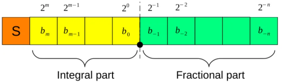
Figure 2.1: Qm,n format with m-bit integral part and n-bit fractional part.

Depending on implementations, Ixˆ may be stored in two’s complement

represen-tation, or as a sign-bit and an absolute value. When the binary point, determined by the scaling factor, falls in the middle of the representation, digits are partitioned into

integral and fractional parts, depending on their position. A fixed-point format with m-bit integral part and n-bit fractional part is often written Qm,n (see Figure 2.1).

Fixed-point arithmetic is implemented on top of integer arithmetic. Explicit rescaling operations must be performed to ensure compatibility of operands, control word-length or avoid overflows. For example, consider the (unsigned) fixed-point

addition of v1 = 2−1 × 10011b and v2 = 2−3 × 01101b. A custom word-length

implementation is illustrated in Figure 2.2. The two numbers must first be aligned

be to the same exponent by scaling v2 down by two positions, which leads to the

truncation of its two least significant bits. Finally, a sixth, guard bit is used to account for bit-growth and prevent overflows. This is not the only solution: for example, both operands could be further shifted by one position to keep output wordlength under 6 bits, or rounding could be used instead of truncation to improve error bounds.

Binary point position

1 0 0 1 1

0 1 1 0 1

+

1 0 1 1

0

0

=

Figure 2.2: Fixed-point addition of two 5-bit numbers.

Fixed-point multiplication illustrates well the challenges of fixed-point arith-metic. Consider the product v1×v2, with v1, v2 defined as in the previous paragraph.

No alignment is required to perform the operation, as:

v1 × v2 = (2−1× 10011b) × (2−3× 01101b) = 2−4× (10011b × 01101b).

The result can thus be computed without loss of accuracy, irrelevant of the scaling factors. However, fixed-point multiplication of same word-length numbers produces a result of double width, which can lead to a phenomenon sometimes called bit-width explosion. Additional truncations or roundings, called quantizations, must be introduced to avoid this problem. This leads to computational errors whose magnitude depends on the computation and the severity of the quantizations.

2.2.2 Floating-Point Arithmetic

Contrary to fixed-point arithmetic, where scaling factors are implicitly encoded in the computation, floating-point arithmetic uses explicit exponents in the represen-tation itself in order to automatically scale to different ranges of values. It can be

Table 2.1: Interpretation of a IEEE 754 Floating-Point Number

Exponent Value T Interpretation Remark

e = emin 0 (−1)S _{× 0}

e = emin �= 0 (−1)S_{× 2}e_{× 0.T Denormal numbers}

emin + 1 ≤ e < emax any (−1)S_{× 2}e_{× 1.T Normal numbers}

e = emax 0 (−1)S_{× ∞ Infinities}

e = emax �= 0 NaN “Not a Number”

seen as a form of binary scientific notation. For example, whereas chemists refer to the Avogadro constant as:

6.02214086 × 1023mol−1, it can also be written in binary form as:

1.11111110000110000101111 × 101001110_mol−1_.

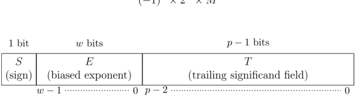
More formally, a floating-point number consists in a sign bit S, a signed exponent E and a fixed-point number M with 1-bit integral part, called the mantissa or significand. The represented value is:

(−1)S× 2E × M S (sign) E (biased exponent) T

(trailing significand field)

1 bit w bits p− 1 bits

w− 1 0 p − 2 0

Figure 2.3: Binary Representation of a IEEE 754 Floating-Point Number Most floating-point implementations are based on the IEEE754 standard and use the binary representation pictured in Figure 2.3. This encoding saves 1 bit by not storing the integral part of the significand, but inferring it from the fractional part and the exponent. The interpretation, detailed in Table 2.1, assumes that (most) floating-point numbers are stored in so-called normal form, which also ensures that they are represented with a maximum number of significand bits. The exponent e is

stored as a biased integer e� _{such that e = e}� _{− 2}w−1_{+ 1 . We write e = emin when}

e� _{= 0, and e = emax when e}� _{= 2}w_{− 1}

While floating-point arithmetic can be emulated on top of integer arithmetic, performance is prohibitive. Consequently, most implementations rely on dedicated hardware support, usually in the form of a Floating-point Processing Unit (FPU), off-the-shelf operators or as a custom datapath.

2.2.3 Comparison

In the following, we discuss the main differences between fixed-point and floating-point arithmetic with respect to programmability, hardware cost, availability and numerical properties.

Programmability

To the programmer or hardware designer, floating-point arithmetic offers many ad-vantages in terms of simplicity, as floating-point hardware automatically performs necessary rescalings to maximize accuracy and minimize the risk of overflows.

In contrast, programming in fixed-point arithmetic often implies dealing with such problems manually. For example, multiplying two 8-bit unsigned fixed-point numbers, with respective exponents −2 and −4, may be written in C:

uchar8 mul_2_4 ( uchar8 a , uchar8 b ) {

r e t u r n ( a >> 4 ) ∗ ( b >> 6 ) ; }

The programmer must manually keep track of the implicit factor of each datum in order to perform the right operation.

Libraries such as SystemC (OSCI), ac_fixed (Mentor Graphics) and ap_fixed (Xilinx) can handle some of these concerns for the hardware designer by performing automatic rescalings given the format of operands. However, fine-grained control of wordlength often requires the introduction of manual quantizations, expressed as intermediary variables which clutter the specification with implementation details. Area Cost and Power Consumption

Floating-point hardware implementations are significantly more costly than fixed-point implementations. For example, floating-fixed-point adders require pre-alignment logic (usually in the form of expensive barrel shifters), adder/rounding logic and normalization logic with leading-zero detection. This makes floating-point arith-metic prohibitive for area-constrained applications. Power usage of floating-point operators is also typically higher than that of integer operators used in fixed-point arithmetic.

Availability

Because of their significant hardware cost, many embedded processors do not even feature FPUs. On these platforms, the use of fixed-point arithmetic is virtually mandatory.

Numerical Properties

In fixed-point arithmetic, the scaling factor is the weight of the least significant bit and corresponds to the smallest non-zero representable value, also called quantization step. Along with wordlength, it determines the range of representable numbers. For

-1.5e+06 -1e+06 -500000 0 500000 1e+06 1.5e+06 0 0.02 0.04 0.06 0.08 0.1 0.12 0.14 0.16 Represented Value Maximum Error

Absolute Error in Single-Precision Floating-Point

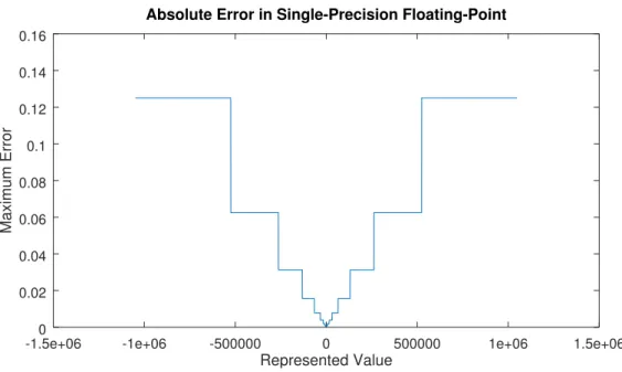
Figure 2.4: Maximum representation error of floating-point numbers as a function of represented value.

example, the b = (m + n + 1)-bit Qm,n format has quantization step 2−n and covers

the range:

[−2b−n−1, 2b−n−1− 1].

This interval can be extended by increasing the size b of the representation or choos-ing a coarser quantization step. This necessary trade-off between range and accuracy is a major disadvantage of fixed-point arithmetic.

In contrast, floating-point formats feature a variable exponent which allows them to represent a wide interval of numbers. Specifically, the range of (normalized) non-negative values that can be represented by a b = (w + p)-bit IEEE754 floating-point number is:

[2−(2w−1−2), 22w−1 − 22w−1−p]

Small values are encoded with a small exponent and considerable accuracy, while bigger exponents allow very large values to be represented, albeit possibly with larger errors. In other words, while fixed-point numbers have a fixed quantization step and bounded absolute errors, floating-point has quantization steps proportional to magnitude of numbers and bounded relative errors. Floating-point quantization step size as a function of number magnitude is plotted in Figure 2.4.

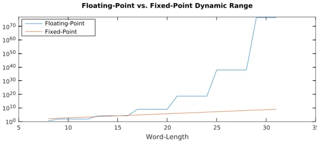
The notion of dynamic range can be introduced to summarize these properties. Dynamic range is defined as the ratio between the smallest and largest representable values and does hence not depend on the scaling factor of fixed-point formats. Dy-namic range of fixed-point and floating-point formats are plotted in Figure 2.5 as a function of wordlength. We can observe that for very small bit-widths, fixed-point numbers actually offer a larger dynamic range. But as wordlength increases, this phenomenon is reversed and floating-point arithmetic gives much more flexibility.

100 1010 1020 1030 1040 1050 1060 1070 5 10 15 20 25 30 35 Word-Length Floating-Point vs. Fixed-Point Dynamic Range Floating-Point Fixed-Point

Figure 2.5: Dynamic range of floating-point and fixed-point representation as function of wordlength. Floating-point exponents of �25%� of wordlength are as-sumed.

2.2.4 Summary

Floating-point arithmetic is more versatile than fixed-point arithmetic and offers better numerical properties, with a wide range of representable values and small relative errors. Unfortunately, its significant hardware cost hinders its adoption in many embedded contexts and fixed-point arithmetic must then be used.

2.3

Floating-Point to Fixed-Point Conversion

As many DSP processors lack support for floating-point arithmetic, or because of its significant area cost in FPGA and ASIC designs, many applications must be implemented in fixed-point. Unfortunately, programming in fixed-point arithmetic is a challenging task as overflows and numerical errors may significantly degrade accuracy. For this reason, these concerns are usually addressed at a later design stage: the application is specified and validated in floating-point arithmetic, before being converted to fixed-point.

In this section, we discuss the problem of floating-point to fixed-point conversions. We then expose the techniques available to address this problem automatically, with a focus on accuracy evaluation, a step that often is the bottleneck of the process.

2.3.1 Problem Setup

The intent of float-to-fix is to assign to each value in a computation a fixed-point format minimizing the risk of overflow and ensuring that enough accuracy is re-tained with respect to the reference implementation/specification. That specifica-tion may be given as a block diagram, Signal Flow Graph (see Secspecifica-tion 2.4.1), or as a C/C++/Matlab source code.

Preventing overflows is usually achieved by performing range analysis on the input specification: the interval of each value (i.e., each signal in the graph, or each variable in the program) is determined in order to allocate enough bits in the most significant positions. Word-lengths are then adjusted until a suitable trade-off is found between performance/cost and accuracy. Depending on the context and target platform, the problem being solved can be stated differently:

• In a software/DSP setting, the challenge consists in finding a fixed-point spec-ification that i) meets (or exceeds) accuracy requirements, ii) can be imple-mented using available CPU primitives.

The design space is thus limited by the word-lengths and instructions proposed by the target processor.

• In a hardware design setting, floating-point to fixed-point conversion takes the form of a Word-Length Optimization, where one tries to minimize area cost or maximize accuracy, subject to some accuracy or cost constraint.

The design space is usually considerably larger than in software fixed-point, as the datapath can be fine-tuned to arbitrary word-lengths. WLO problems are combinatorial in nature. It has been shown that a restricted analytical form of the multiple wordlength assignment problem is of NP-hard complexity [2]. Let w denote a fixed-point configuration, λ(w) the associated error and C(w) the cost estimate of that implementation. We distinguish two forms of WLO problems. The accuracy maximization problem may be stated as:

max

w λ(w) subject to C(w) ≤ Cmax

and the cost minimization problem as: min

w C(w) subject to λ(w) ≤ λmax

These optimization problems can be solved using combinatorial optimization algo-rithms, or a more ad-hoc, semi-manual exploration. At a high-level, all approaches

boil down to the same idea: starting from an initial configuration w0, the current

solution is iteratively refined to optimize the objective function. At each step, the cost C(w) and accuracy λ(w) are evaluated and a new configuration is chosen until some acceptance condition is reached (for example, the absence of progress), or until the designer in charge of the conversion is satisfied with the results.

To perform this optimization automatically and reach a good solution in rea-sonable time, sufficiently fast methods are required for evaluating the cost and ac-curacy of a design. Cost estimation is a challenging task, as the actual cost may depend on decisions made by the design tool after float-to-fix conversion, such as operator-sharing. In practice, more-or-less comprehensive high-level cost estimates are used [3, 4].

While quantization noise can negatively impact the behavior of the system, over-flows have an even stronger consequences on numerical correctness. Word-Length Optimization is mostly focused in tweaking the size of the fractional part of fixed-point operands to approach the optimal solution. However, before entering the

optimization loop, it is necessary to determine the size of the integral part, in order, depending on the criticity of the application, to limit or the risk or guarantee the absence of overflows. This analysis is called range estimation.

2.3.2 Range Estimation

In order to avoid overflows, it is necessary to ensure that the range of values spanned by each variable during the computation does not exceed the capacity of its repre-sentation. This range naturally depends on inputs and can be estimated from their own range or from representative samples.

When input range is known, any static analysis designed to compute safe variable bounds can be used. Interval or Affine Arithmetic have been extensively applied to this problem. Affine arithmetic can model exactly range propagation through a linear non-recursive program, but non-linearity or the presence of feedback loops gives rise to approximations.

For LTI systems, the L1 _{norm of the transfer function (which can be computed by}

hand, or automatically from an adequate representation) gives precise information on the range of outputs. David Cachera and Tanguy Risset proposed a formal approach based on the polyhedral model and the (max, +) tropical algebra to compute ranges on affine loop nests operating on uni-dimensional arrays [5].

In general, without stringent restrictions on the nature of the system, any safe static method is bound to produce pessimistic over-approximations: computing the precise semantics of a program is an undecidable problem. Moreover, even when error bounds can be determined exactly (for example, using affine arithmetic in a basic block with linear operations), numbers close to the minimum or maximum values are unlikely to be observed in practice, as they correspond to statistical extremes.

As a constrained example, consider the addition of 5 independent uniform ran-dom variables ranging over interval [0, 1]. Their sum is obviously distributed over interval [0, 5]. However, as evident from the plot of its probability density function (see Figure 2.6), values over 4 are unlikely to be observed - in fact, the probability is less than 1%. One may choose to use saturating arithmetic and only assume values less than 4, without significantly affecting the results of the computation. However, purely static methods are unlikely to help the designer to recognize such situations. Except in critical systems, where overflows are not acceptable, simulation is thus often preferred, or used in complement, to static analyses: provided that inputs are in a sufficient number and statistically representative, measured bounds indirectly reflect signal characteristics, and are thus often much more tight than those obtained with static approaches.

2.3.3 Accuracy Metrics

Formulating an accuracy constraint supposes the choice of a particular metric to characterize performance degradations. Two main classes of metrics may be used: “Hard” metrics (error bounds) In critical systems, accuracy constraints are

usu-Figure 2.6: PDF of the sum of 5 i.i.d random variables with distribution U ([0, 1]).

ally specified as a hard bounds on error. Typically: |e| = |ˆx − x| < ε

Statistical metrics In signal and image processing systems, soft metrics based on the statistics of signals are usually used. The most common one is called noise power and involves the first and second statistical moments of the error, seen as a random noise e:

P (e) = E(e2) = µ2_e + σ_e2

where µe and σe2 denote the mean and variance of variable e. Noise power is

generally given in decibels (dB):

Plog(e) = 10 log10P (e) dB.

A related way to measure the relative magnitude of signals and errors is the Signal to Quantization Noise Ratio (SQNR). It is defined as:

SQNR = Plog

� Signal

Error �

= Plog(Signal) − Plog(Error)

Signal power Plog(Signal) is generally known from representative inputs.

Com-puting noise power or SQNR is thus equivalent.

Finally, whereas in noise power, only the first two moments are used, estimates of higher-order moments give more information on the shape of the probability distribution and can be used to define even more fine-grained constraints [6]. However, in the following, we will mostly consider noise power, as noise power and SQNR are the most widely used metrics.

2.3.4 Accuracy Evaluation

Accuracy evaluation is the process of evaluating the accuracy degradation occasioned by a fixed-point implementation.

Simulation

Given a fixed-point specification w, the obvious way to determine its accuracy is to perform bit-accurate fixed-point simulations with representative inputs and compare the results with the reference implementation. This approach produces reliable estimates and is easy to implement for any computation. However, it is also very time-consuming:

• Compared to floating-point or native integer operations, fixed-point simula-tions suffer from a large performance hit on general purpose hardware.

• To produce reliable estimates of statistical metrics, this process must be re-peated a large number of times to determine the statistical moments of the error with enough confidence.

Since accuracy evaluation is performed at every WLO step, the use of simulations is often a bottleneck limiting the depth of the design space exploration, leading to suboptimal implementations

Analytical Approaches

In analytical methods, an accuracy model of the specification is constructed prior to WLO to avoid simulations and speed up accuracy evaluation. While the construc-tion of the model may be relatively costly, it can be used to quickly determine the accuracy of any solution, thus considerably increasing the number of optimization steps that can be performed.

2.4

Analytical Accuracy Evaluation

Our contributions, exposed in the next chapter, focus on analytical accuracy evalu-ation. The principle of analytical accuracy evaluation is to derive an accuracy model from a floating-point specification. The statistical moments of quantization errors, viewed as random variables, are propagated through the computation to construct a symbolic expression of overall noise power at the output of the system.

Two kinds of model are required: first, the statistical properties of quantization errors need to be determined. Secondly, the overall impact of the system on these errors at the output must be captured by abstract models.

Current methods operate on dataflow models such as Signal Flow Graphs as an intermediate representation of the system (Section 2.4.1). These graphs are trans-formed with simple rewrite rules to introduce error sources (Section 2.4.2) repre-senting quantization errors as additional inputs. Quantization noise models (Sec-tion 2.4.3) provide expressions for the mean and variance of these errors as a func(Sec-tion of input and output precisions. The challenge then consists in constructing a noise

formula representing the moments of errors at the output of the system. A variety techniques have been proposed to achieve this goal, with different assumptions on the system. They are discussed in the rest of this section.

2.4.1 Signal-Flow Graphs

Signal Flow Graphs [7] (SFGs) are a flavor of synchronous data flow [8] graphs used in the signal processing community to model discrete computations. Semantically, each node in a SFG represents a sequence of values, defined in terms of the node’s predecessors. In particular, SFGs contain explicit delay operations, in the form of

“register” nodes (usually marked z−1_{): at any point in time, the output of these}

nodes is defined as their input at the previous clock cycle.

As an example, an SFG for a Finite Impulse Response (FIR) filter is shown in Figure 2.7. The input sequence x(n) is delayed through a series of register nodes which can collectively be seen as a shift register. The output y(n) is defined as the dot product of the content of the shift register and a vector of coefficients (bi)0≤i≤3.

Alternatively, SFG nodes may be expressed as recurrence equations. For exam-ple, the SFG in Figure 2.7 is a graphical representation of the following system:

               y(n) = m3(n) + p2(n) m2(n) = b2δ2(n) p2(n) = m2(n) + p1(n) m3(n) = b3δ3(n) p1(n) = m1(n) + m0(n) δ3(n) = δ2(n − 1) m0(n) = b0x(n) δ2(n) = δ1(n − 1) m1(n) = b1δ1(n) δ1(n) = x(n − 1)

SFGs are schedulable if any cycle contains at least one delay node, while graphs with 0-weight cycles do not represent any meaningful system. An SFG verifing this condition is unambiguously defined modulo initial conditions – the state of the system before the beginning of the computation. This validity condition may be seen as a restriction of the conditions [9] given by Karp, Miller and Winograd for a system of uniform recurrence equations to be explicitly defined.

z−1 z−1 z−1 b1 b2 b3 b0

+

+

+

Figure 2.7: SFG of a FIR Filter computing the formula: y(n) =�3_i=0bix(n − i). Nodes labeled z−1 represent one-cycle delays and triangle-shaped nodes multipli-cation by a constant coefficient.

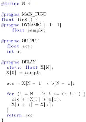
#d e f i n e N 4 #pragma MAIN_FUNC f l o a t f i r 8 ( ) { #pragma DYNAMIC [ −1 , 1 ] f l o a t sample ; #pragma OUTPUT f l o a t a c c ; i n t i ; #pragma DELAY s t a t i c f l o a t X[N ] ; X [ 0 ] = sample ; a c c = X[N − 1 ] ∗ b [N − 1 ] ; f o r ( i = N − 2 ; i >= 0 ; i −−) { a c c += X[ i ] ∗ b [ i ] ; X[ i + 1 ] = X[ i ] ; } r e t u r n a c c ; }

Figure 2.8: FIR filter implementation for the Id.Fix conversion tool.

Some tools such as Id.Fix [10] build a SFG out of a annotated C program. After WLO, a C/C++ fixed-point implementation, using the ac_fixed library, is output. There are two main advantages to this approach. First, a source code implementation is more easily integrated into a custom validation framework than a SFG or a block diagram. Perhaps more importantly, this technique can be used in a HLS context, with WLO viewed as a source-to-source transformation. In Figure 2.8, an implementation of the FIR filter in Figure 2.7 is given, as accepted by Id.Fix:

This code actually represents one iteration of the FIR. After parsing, the control flow of the top function (marked by the MAIN_FUNC pragma) is fully flattened and an acyclic data flow graph is built with a producer-tracking simulation. Finally, the

DELAY pragma helps the tool insert the delay nodes, corresponding to dependences

across consecutive function calls.

2.4.2 Error Sources

In a fixed-point implementation, an arithmetic operator can introduce multiple er-rors: inputs may need to be quantized to fit the operator’s format and the precision of the output may also be reduced to limit bit-width growth.

Quantizations may be expressed explicitly as additional operations, as shown in Figure 2.9. In analytical accuracy evaluation, though, round-off errors are modeled as additive noise perturbating an infinite-precision signal. This is usually reflected through a graph transformation: each quantization is replaced with an addition

x y + z Q 0 Q1 Q2 ≡ x y + z + e0 + e1 + e2

Figure 2.9: Introduction of error sources in a Signal Flow Graph.

between the original signal and the quantization error. The virtue of this transfor-mation is to reframe quantization errors as new system inputs, which can be modeled as a stochastic process known as Pseudo Quantization Noise (PQN).

2.4.3 Pseudo Quantization Noise model

Analytical accuracy evaluation seeks to predict the influence of quantization errors on the output of the system. At first, this may appear like an infeasible task, since actual errors depend on system inputs. As it turns out, in the vast majority of cases, quantization errors can be statistically characterized from the precision of the original and quantized signals, and the mode of quantization (truncation, rounding or convergent rounding). Moreover, this Pseudo Quantization Noise is uncorrelated from the input signal and other error sources, which further simplifies the analysis.

For example, consider the truncation of some infinite-precision signal x to x�_,

with quantization step q = 2−n_{. We have:}

x� = x + ex

with error ex = x�− x within the interval:

I =] − q; 0[.

It can be shown [11] that, if quantization step q is sufficiently small, ex can be

modeled as uniformly distributed variable: ex ∼ U(I)

such that signal x and quantization noise ex are uncorrelated. We can thus give the

mean and variance of the error:

E(ex) = −q/2 Var(ex) =

q2

12

The model above captures the distribution of errors as a continuous probabil-ity distribution, and is thus suitable for modeling the quantization of an infinite-precision (analog, floating-point) signal to fixed-point infinite-precision. Using rounding

instead of truncation leads to a similar model with I = (−q/2; q/2] and E(ex) = 0,

whereas discrete distributions can be used to characterize round-off errors between fixed-point formats [12]. Noise models for different configurations are shown in Fig-ure 2.10.