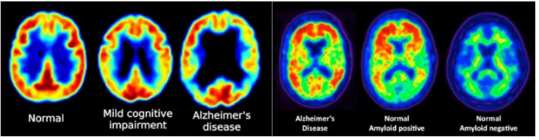
Classification of Alzheimer's Disease and Mild Cognitive Impairment Using Longitudinal FDG-PET Images
114
0
0
Texte intégral
Figure


+7

Documents relatifs
