FORWARD AND INVERSE MODELLING OF MAGNETIC INDUCTION TOMOGRAPHY (MIT) FOR BIOMEDICAL APPLICATION
AMIR AHMAD ROOHI NOOZADI D´EPARTEMENT DE G´ENIE PHYSIQUE ´
ECOLE POLYTECHNIQUE DE MONTR´EAL
TH`ESE PR ´ESENT´EE EN VUE DE L’OBTENTION DU DIPL ˆOME DE PHILOSOPHIÆ DOCTOR
(G´ENIE PHYSIQUE) MARS 2017
c
´
ECOLE POLYTECHNIQUE DE MONTR´EAL
Cette th`ese intitul´ee :
FORWARD AND INVERSE MODELLING OF MAGNETIC INDUCTION TOMOGRAPHY (MIT) FOR BIOMEDICAL APPLICATION
pr´esent´ee par : ROOHI NOOZADI Amir Ahmad
en vue de l’obtention du diplˆome de : Philosophiæ Doctor a ´et´e dˆument accept´ee par le jury d’examen constitu´e de :
M. FRANCOEUR S´ebastien, Ph. D., pr´esident
M. YELON Arthur, Ph. D., membre et directeur de recherche M. M´ENARD David, Ph. D., membre et codirecteur de recherche M. LEBLOND Fr´ed´eric, Ph. D., membre
DEDICATION
ACKNOWLEDGMENT
I would like to thank my advisers, Arthur Yelon and David M´enard, for their consistent sup-port and inspiration. It was a pleasure working with these two brilliant scientists.
I would also like to thank Herv´e Gagnon for fruitful discussions, technical consultant and helpful suggestions. Herv´e expertise had a noticeable effect on the progress rate of this re-search.
I thank the members of the jury S´ebastien Francoeur, Fr´ed´eric Leblond, and Andy Adler for evaluating this thesis and for their constructive comments.
I would like to thank my former supervisors Reza Jafari and Shahram Jalalzadeh for their supports and fruitful discussions since I started studying physics till the day this thesis was submitted.
I thank all my colleagues and friends, especially Nima Nateghi, Saeed Bohloul,
Mehran Yazdizadeh, Antoine Morin, Nicolas Teyssedo, Sahar Fazeli and Saman Choubak, for their support and helpful discussions.
And finally I thanks my wonderful Mom, Dad, and my sister Ely for their continuous support and endless love.
R´ESUM´E
Cette th`ese d´eveloppe un outil de simulation destin´e au design d’instruments de tomographie par induction magn´etique (MIT pour Magnetic Induction Tomography). Ce simulateur per-met d’investiguer la possibilit´e d’utiliser la m´ethode d’imagerie par tomographie par induction magn´etique afin de faire la conception d’un dispositif sans-contact capable de d´etecter une h´emorragie `a l’int´erieur du crˆane humain. La m´ethode sp´ecifique de calcul num´erique utili-s´ee pour la simulation du dispositif de mˆeme que le calcul de la sensibilit´e avec la m´ethode directe (introduite dans cette th`ese) et la r´esolution du probl`eme inverse, qui reconstruit une carte de la conductivit´e `a partir des r´esultats de simulation, sont optimis´es afin de simuler un dispositif op´erant `a 50 kHz. Ce dispositif est capable de d´etecter le changement de la conductivit´e dans une gamme se rapprochant de celle des tissus biologiques.
Le fonctionnement de base de la tomographie par induction magn´etique repose sur les mesures des propri´et´es ´electromagn´etiques dites passives telles que la conductivit´e. L’utilisation d’une telle m´ethode pour d´etecter les h´emorragies c´er´ebrales se justifie par le fait que la conductivit´e du sang est plus ´elev´ee que la conductivit´e des autres tissus constituant le cerveau. Une autre application potentielle de cette m´ethode est le suivi en temps r´eel, de mani`ere non invasive, de l’alt´eration des tissus qui peut s’observer `a partir d’un changement de conductivit´e, par exemple les probl`emes respiratoires, la gu´erison de plaies ainsi que les processus isch´emiques. Les bobines d’induction dans le dispositif de tomographie par induction magn´etique pro-duisent un champ magn´etique primaire dans la r´egion d’int´erˆet (ROI pour Region of Interest) et ce champ alternatif induit des courants alternatifs (courants de Foucault) dans les r´egions conductrices. Ces courants induits produisent `a leur tour un champ magn´etique secondaire dans la r´egion d’int´erˆet. Ce champ magn´etique secondaire produit un champ aux bobines de r´eception qui est utilis´e pour reconstruire la distribution de la conductivit´e dans la r´egion d’int´erˆet.
Un d´efi important concernant l’´etat de l’art de ces dispositifs est la d´etection du signal se-condaire en pr´esence du signal primaire, qui est plusieurs ordres de grandeur plus fort. Le dispositif pr´esent´e utilise une g´eom´etrie pour l’induction et la d´etection sp´ecialement con¸cue pour op´erer dans les basses fr´equences avec un ratio signal sur bruit acceptable de mˆeme qu’une configuration du d´etecteur qui est moins sensible au champ primaire. La m´ethode directe du calcul de la matrice de sensibilit´e introduite dans cette th`ese nous fournit une m´ethode num´erique robuste pour la reconstruction d’images, ce qui r´esulte en une qualit´e d’image sup´erieure par rapport aux autres m´ethodes propos´ees dans la litt´erature.
6 bobines d’excitation concentriques qui sont plac´ees `a diff´erentes hauteurs sur la surface externe. Ces bobines produisent un signal primaire dont la majorit´e des lignes de champ sont parall`eles `a l’axe principal du cylindre o`u est plac´e l’objet d’int´erˆet. Ce champ induit alors des courants de Foucault (courants de conduction et courants de d´eplacement) dans les r´ e-gions conductrices, ce qui g´en`ere un champ magn´etique secondaire. Ce champ secondaire est d´etect´e par 80 bobines de r´eception (16 rang´ees de d´etecteurs plac´es `a 5 hauteurs diff´erentes) qui sont plac´ees sur les parois du cylindre de mani`ere perpendiculaire au plan des bobines d’excitation.
La simulation de ce dispositif n´ecessite un mod`ele math´ematique comprenant le probl`eme direct et le probl`eme inverse. Le probl`eme direct est la simulation math´ematique du syst`eme, qui r´esout les ´equations de Maxwell dans la r´egion d’int´erˆet avec les conditions fronti`ere ad´ e-quates.
Le probl`eme impliquant les courants de Foucault est r´esolu par l’utilisation d’un mod`ele connu sous le nom d’´equations de Maxwell compl`etes (traduction libre de full Maxwell’s equations). Ce probl`eme est r´esolu par la m´ethode des ´el´ements finis (´el´ements en p´eriph´erie, traduction libre de edge elements) en consid´erant les fonctions de Whitney de premier ordre. Le mod`ele est compar´e `a des solutions analytiques connues pour des g´eom´etries simples. Le probl`eme direct nous permet d’obtenir l’amplitude des champs magn´etiques et ´electriques qui sont d´etectables, la distribution et l’ordre de grandeur des courants de Foucault ainsi que le changement de phase du champ magn´etique d´etect´e qui est caus´e par la partie conductrice de la r´egion d’int´erˆet.
`
A partir du probl`eme direct, la matrice de sensibilit´e peut ˆetre extraite, ce qui est n´ eces-saire afin de r´esoudre le probl`eme inverse. Les m´ethodes disponibles pour extraire la matrice de sensibilit´e, par exemple le th´eor`eme de r´eciprocit´e de Geselowitz, sont g´en´eralement des formulations ind´ependantes du probl`eme direct consid´er´e. Cependant, pour notre mod`ele, la sensibilit´e est calcul´ee directement par la diff´erentiation num´erique de l’´equation d’Helmholtz par rapport aux propri´et´es ´electriques. Cette m´ethode pour calculer la matrice de sensibilit´e (la m´ethode directe) est introduite dans cette th`ese et les r´esultats de la reconstruction pour cette m´ethode sont compar´es avec ceux provenant du th´eor`eme de r´eciprocit´e appliqu´e aux probl`emes de tomographie par induction magn´etique. La matrice de sensibilit´e peut r´ev´eler `
a quel point la sensibilit´e d’une partie de la r´egion d’int´erˆet peut ˆetre affect´ee par un change-ment quelconque de courant ou de conductivit´e (de mˆeme que pour d’autres propri´et´es). De plus, extraire la matrice de sensibilit´e permet de calculer la direction de sensibilit´e maximale `
a un changement de conductivit´e dans une certaine partie de la r´egion d’int´erˆet, ce qui per-met de d´eterminer le meilleur arrangement et emplacement des d´etecteurs. L’extraction de la matrice de sensibilit´e par la m´ethode directe, `a partir des outils permettant de r´esoudre
ce mod`ele, n’est pas une tˆache simple. Ainsi, le mod`ele direct doit ˆetre d´evelopp´e dans son enti`eret´e dans MATLAB.
Le probl`eme inverse (la description de la structure interne du syst`eme fournie par des don-n´ees indirectes) est ensuite r´esolu `a l’aide de la matrice de sensibilit´e et des m´ethodes dispo-nibles dans la litt´erature (ces m´ethodes sont courantes pour la tomographie par imp´edance ´
electrique). Pour le probl`eme inverse, r´esolu par la m´ethode du maximum a posteriori, les approches lin´eaires et non lin´eaires ont ´et´e utilis´ees afin de reconstruire la conductivit´e. L’ap-proche lin´eaire est prometteuse pour l’imagerie diff´erentielle afin de confirmer l’apparition d’une l´esion si nous disposons au pr´ealable d’informations concernant la conductivit´e nor-male de la tˆete et du crˆane. Cependant, l’approche lin´eaire am`ene `a des valeurs erron´ees de la conductivit´e. L’approche non lin´eaire a ´egalement ´et´e impl´ement´ee afin de permettre le calcul de la valeur absolue de la conductivit´e sans aucune information pr´ealable. Toutefois, l’approche non lin´eaire est coˆuteuse au point de vue des ressources computationnelles et donc faire la tomographie par induction magn´etique en utilisant notre m´ethode n’est pas envisa-geable pour calculer la valeur absolue de la conductivit´e.
La configuration des senseurs adopt´ee pour notre dispositif, dont le positionnement des cap-teurs est perpendiculaire aux bobines d’excitation, am`ene un avantage au point de vue de la soustraction du champ primaire, ce qui est un d´efi constant dans l’op´eration des autres dispositifs de ce type. Les signaux ont ´et´e simul´es pour diff´erentes hauteurs de disque dans le cylindre et diff´erentes locations de la l´esion `a l’int´erieur du disque. La distribution de la conductivit´e est ensuite reconstruite `a partir du changement de voltage induit dans les sen-seurs.
Les r´esultats du probl`eme de reconstruction concernant le mod`ele du disque dans le dispositif propos´e, en consid´erant que le niveau de bruit est constant et vaut 1% du signal maximal d´etect´e, montrent un ratio de signal sur bruit de 40 dB. Les capteurs magn´etiques utilis´es pour construire ce dispositif devraient ˆetre capables de d´etecter des champs de 10 pT avec ce mˆeme ratio signal sur bruit.
ABSTRACT
This thesis develops a simulation package for the design of Magnetic Induction Tomogra-phy (MIT) instruments and exploit the simulator to investigate the possibility of using the magnetic induction tomography imaging method to design a non-contact device capable of detecting a blood hemorrhage inside the skull. The specific numerical method (full Maxwell’s equation) used for simulation of the device, followed by calculation of the sensitivity with the direct method (introduced in this dissertation) and a regularized inverse solver which re-construct the conductivity map from the simulation outputs (magnetic field), are optimized to simulate a device operating at 50 kHz. This device is capable of detecting the change in conductivity in ranges close to biological tissues.
MIT operates based on the measurement of passive electromagnetic properties such as con-ductivity. The rationale behind using this method for detecting cerebral stroke is based on the fact that the conductivity of the blood is larger than that of the other tissues in the head. Other potential medical applications for this device are real-time, non-invasive monitoring of tissue alterations which are reflected in the change of the conductivity, e.g. ventilation disorders, wound healing and ischemic processes.
The inductive coils in the MIT device produce a primary magnetic field in the region of interest (ROI) and this alternating magnetic field induces alternating (eddy) currents in the conductive regions. These eddy currents, in turn, generate a secondary magnetic field in the ROI. This secondary magnetic field generates a field at the receivers, which is used to reconstruct the conductivity distribution of the ROI.
An important challenge in the state of art devices is the detection of the secondary signal in the presence of the primary signal, which is orders of magnitude stronger. The device uses a geometry in induction and detection designed to operate in low frequencies with ac-ceptable SNR and detector configuration that is least sensitive to the primary field. The direct method of calculating the sensitivity matrix introduced in this thesis provides us with a robust numerical method for image reconstruction which results in superior image quality compared to other proposed methods in the state of the art.
The proposed configurations involves a cylindrical shape device with 6 concentric excitation coils which are located at different heights on the outer surface of the cylinder. These coils produce a primary magnetic field with majority of the field lines parallel to the main axis of the cylinder, where we position the object of interest. This primary field induces eddy currents (conduction and displacement current) in the conductive regions of the ROI, which generate a secondary magnetic field. The secondary magnetic field is detected in 80 sensors
(16 arrays of sensors at 5 different heights), which are located on the cylinder walls perpen-dicular to the plane of excitation coils.
The simulation of this device requires a mathematical model consisting of a forward and an Inverse problem. The forward problem is the mathematical simulation of the device, which solves Maxwell’s equations in the ROI with the appropriate boundary conditions.
The problem is known as the eddy current problem is solved using a model known as full Maxwell’s equations. The eddy current problem is solved using a finite element method (edge basis) considering the first order Whitney functions. The model is bench-marked with avail-able analytic solutions for known geometries. The forward problem provides us with the magnitude and direction of the detectable magnetic and electric field, eddy current size and distribution and also the phase change in the detected magnetic field, which is caused by the conductive area in the ROI.
From the forward problem, the sensitivity matrix is extracted that is used in solving the reconstruction problem. Methods available for extracting the sensitivity matrix, like using the Geselowitz reciprocity theorem, are mainly independent formulations regardless of the method used in solving forward problem. However, in our model, the sensitivity is directly calculated by the rigorous numerical differentiation of the governing equation (Helmholtz) in the forward problem, with respect to the electrical properties. This method of calculating the sensitivity matrix (the direct method) is introduced in this thesis and the results of re-construction for this method are compared with results from the reciprocity theorem. The sensitivity matrix shows how sensitive is the secondary field of an area in ROI to any change in current or conductivity of other areas (as well as other properties such as permittivity). Furthermore, extracting the sensitivity matrix could allows one to systematically investigate the most sensitive direction to the conductivity change in certain area, at any position in the region of interest to find the the best arrangement and alignment for the sensors. Extracting the sensitivity matrix with the direct method, from available packages which are capable of solving the forward model, is not a straightforward task. Therefore, the forward model is fully developed in MATLAB.
The inverse problem (the description of the internal structure of a system given by indirect data) is then solved using the sensitivity matrix and available methods known for solving inverse problems in the literature (These matrix inversion methods are common with Elec-trical Impedance Tomography). In the inverse problem, which is solved using the maximum a posterior method, both the linear and non-linear approach were taken to reconstruct con-ductivity. The linear approach is promising for differential imaging performed on a head modelled as a disk with different conductivity layers to confirm the appearance of the lesion, if we have prior information about the conductivity of the background (the head and the
skull). However, the linear method will produce an inaccurate conductivity values. The non-linear approach has also been implemented to calculate the absolute value of the con-ductivity without prior information. However, the non-linear method is not computationally cost-wise and therefore performing Magnetic Induction Tomography with using the method is not suitable for calculating the absolute value of the conductivity.
The configuration of the sensors adopted in this device, which is positioning the receivers perpendicular to the excitation coils, makes it advantage in subtraction of the primary signal which has been a main challenge in operation of such devices. The signals were simulated for different height of the disk in the cylinder and different locations of the lesion in the disk model. The conductivity distribution is then reconstructed from the corresponding voltage changes induced in the sensors.
The results of the reconstruction problem performed on the disk model using the proposed device for a constant noise level, which is considered to be 1% of the maximum detected signal, shows a SNR of 40 dB. Magnetic sensors used for building this device should be able to detect 10 pT fields at this SNR.
TABLE OF CONTENTS DEDICATION . . . iii ACKNOWLEDGMENT . . . iv R´ESUM´E . . . v ABSTRACT . . . viii TABLE OF CONTENTS . . . xi LIST OF TABLES . . . xv
LIST OF FIGURES . . . xvi
LIST OF APPENDICES . . . xxi
NOMENCLATURE . . . xxii
CHAPTER 1 INTRODUCTION . . . 1
1.1 Introduction to tomographic impedance techniques . . . 1
1.2 Objectives . . . 3
1.3 Methodology . . . 6
1.3.1 The forward problem . . . 6
1.3.2 The sensitivity matrix (Jacobian) . . . 8
1.3.3 The inverse problem . . . 9
1.3.4 Performing differential imaging of the conductivity . . . 10
CHAPTER 2 STATE-OF-THE-ART IN MIT DEVICES AND POSSIBLE IMPROVE-MENT OF THE PERFORMANCE . . . 12
2.2 Estimation of eddy currents in biological tissues . . . 13
2.3 Possible improvements in the performance . . . 15
2.3.1 Modification in the induction geometry . . . 15
2.3.2 Enhancement of performance in the detection . . . 17
2.3.3 Considerations on the spatial resolution . . . 18
2.4 Proposed device specifications . . . 19
2.4.1 The head model . . . 19
2.4.2 The geometry for induction and detection . . . 21
2.4.3 The number of induction and detection coils . . . 21
2.4.4 The operation frequency . . . 22
2.5 Simulation procedure for primary excitation field and secondary field compu-tation . . . 23
CHAPTER 3 FORWARD PROBLEM FORMULATION FOR MAGNETIC INDUC-TION TOMOGERAPHY . . . 27
3.1 Solutions to Maxwell’s and Helmholtz equations . . . 27
3.1.1 Maxwell’s equations and a proper gauge . . . 27
3.2 Finite element method formulation . . . 31
3.3 Variational formulation . . . 32
3.4 Boundary conditions and the final equation . . . 33
3.5 Edge element basis in 3D . . . 35
3.6 Assembling the global matrix . . . 42
3.7 Validation of the forward problem formulation . . . 43
3.7.1 Long straight wire . . . 43
3.7.2 Helmholtz coils . . . 48
3.7.3 Summary . . . 54
3.8 Visualization of the eddy currents . . . 54
CHAPTER 4 SENSITIVITY MATRIX CALCULATION . . . 59
4.2 Inverse solution of a differential equation . . . 61
4.2.1 Condition of a matrix . . . 61
4.2.2 The inverse MIT problem . . . 62
4.3 The idea of a direct method . . . 62
4.3.1 Extraction of the sensitivity matrix - The direct method . . . 63
4.4 Fast calculation of the sensitivity matrix using the reciprocity theorem . . . . 66
CHAPTER 5 INVERSE PROBLEM FOR MIT . . . 69
5.1 The inverse problem . . . 69
5.1.1 Maximum likelihood estimation . . . 70
5.1.2 Maximum a posteriori estimation . . . 72
5.2 Implementation of maximum a posteriori estimation for a multivariate Gaussian . . . 72
5.3 Iterative Gauss-Newton approach . . . 75
CHAPTER 6 SIMULATION RESULTS . . . 78
6.1 Simulation details . . . 78
6.1.1 Computational details . . . 79
6.2 Secondary field range . . . 82
6.3 Reconstructed targets . . . 83
6.3.1 Most sensitive direction . . . 84
6.4 Case I : Two selected elements . . . 86
6.5 Case II : A disk with two concentric conductive regions . . . 90
6.5.1 Phase change due to modeled cerebral edema development . . . 92
6.5.2 Linear reconstruction of the conductivity map in 2D . . . 94
6.5.3 Linear reconstruction of the conductivity map in 3D . . . 98
6.5.4 Nonlinear reconstruction of the conductivity map in 3D . . . 98
6.5.5 Calculation of the primary and secondary magnetic field . . . 101
6.6 Comparison between two methods of calculating the sensitivity matrix . . . . 106
6.6.1 Comparison of point spread function (PSF) and spatial resolution . . . 109
CHAPTER 7 CONCLUSION AND FUTURE WORKS . . . 114
7.1 Conclusion . . . 114
7.2 Future Work . . . 116
REFERENCES . . . 119
LIST OF TABLES
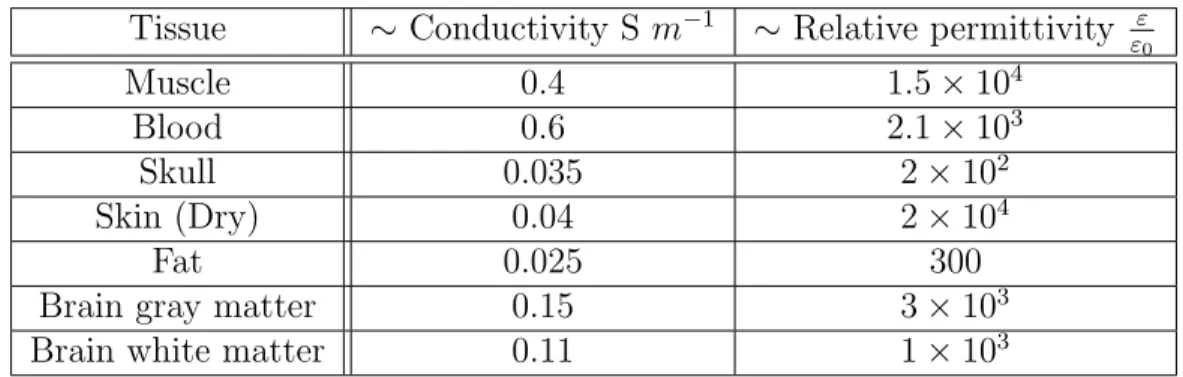
Table 2.1 Dielectric properties (experimental) at 50 kHz (our frequency range of interest for measurements) assigned to each tissue type (Gabriel et al., 1996c,b,a). . . 14 Table 3.1 Numbering of the edges for a single element. . . 36 Table 6.1 Details of meshes used for the forward problem calculations. . . 80
LIST OF FIGURES
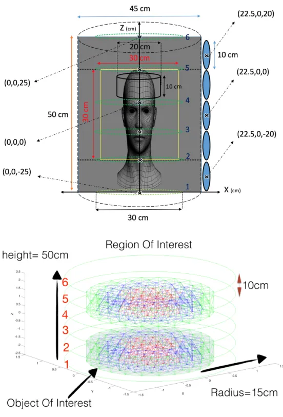
Figure 2.1 Schematic presentation of eddy currents distribution for excitation loops on the sides. Lower density of eddy currents at the center of ROI is due to its’ comparably larger distance from the coils . . . 16 Figure 2.2 Magnetic induction tomography device (top figure) for detection of
haemorrhagic cerebral edema operating at 50 kHz. The position of the excitation coil parallel to the x-y plane (the six round green coils) is specified. One of sixteen detection coils in each row between the excitation currents is shown with their positions (location of the others each can be find by 22.5 degree rotation along the z axis). The yellow square region is the region which we perform the reconstruction of the conductivity. The brain is modeled as a disk with distinct electrical properties (bottom figure) in each layer which will be used as targets in the cylindrical ROI. . . 20 Figure 2.3 Sensor arrangment around the ROI. There are 5 arrays of 16 detecors,
arranged symmetrically on the surface walls of the cylindrical ROI with radius 45 cm and height 50 cm. The distance between the sensor arrays and the surface wall shown in this figure is for clarity. Excitation coils with radius 30 cm are shown in green. . . 24 Figure 3.1 A schematic of all the forward problem boundary conditions. . . 34 Figure 3.2 Defining the first order weighting function on a tetetrahedron and its
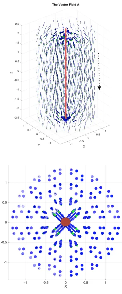
edges. . . 35 Figure 3.3 The magnetic vector potential, A vector field numerically calculated in
temporal gauge for a straight wire in 3D (Side view on the top - Top view on the bottom). . . 45 Figure 3.4 Magnetic field, B vector field numerically calculated for a straight wire
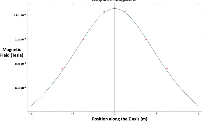
in 3D (Side view on the top - Top view on the bottom). . . 46 Figure 3.5 The analytically calculated magnetic field of a wire (blue) and the
numerically calculated magnetic field of a wire computed at 5 points (red). The average difference is 0.01 % of the analytically calculated value. . . 47
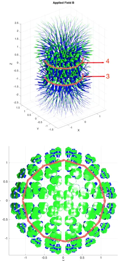
Figure 3.6 The magnetic field Bz calculated using Eq.(3.55) for two coils located
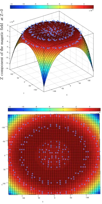
at z = 0.5 (coils 4) and z = −0.5 (coils 3). The indicated values are the points used for validation of the numerical calculations. The points between these two heights are the points with almost uniform magnetic field. . . 48 Figure 3.7 The magnetic field Bz calculated at z = 0 using finite element method
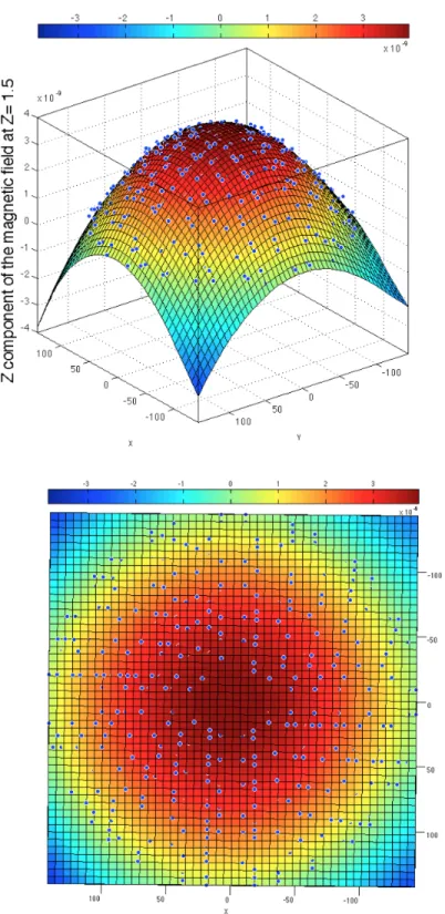
for two coils located at z = 0.5 (coils 4) and z = −0.5 (coils 3). The field is uniform exactly at z = 0 as expected (Side view on the top -Top view on the bottom). . . 50 Figure 3.8 The magnetic field Bz calculated at z = 1.5 using finite element method
for two coils located at z = 0.5 (coils 4) and z = −0.5 (coils 3). The field is nonuniform as we go farther vertically from the coils (Side view on the top - Top view on the bottom). . . 51 Figure 3.9 The numerically calculated magnetic potential, A vector field in
tem-poral gauge for two loops of wire in 3D (Side view on the top - Top view on the bottom). The top view shows that circles are concentric. . 52 Figure 3.10 The numerically calculated magnetic field, B vector field for two loops
of wire (Helmholtz coils) in 3D (Side view on the top - Top view on the bottom). . . 53 Figure 3.11 Conduction currents produced on a disk as the result of inductions from
two coils numerically calculated at different vertical distances from the top and bottom surfaces (Side view on the top - Top view on the bottom). 55 Figure 3.12 Displacement currents produced on a disk as the result of inductions
from two coils numerically calculated at different vertical distances form the top and bottom surface (Side view on the top - Top view on the bottom). . . 56 Figure 3.13 The numerically calculated secondary magnetic potential, A vector
field in temporal gauge produced by eddy currents on the disk sur-face. The side view shows that the vectors curl around the disk (a, b and c are areas with different densities of A) (3D side view on the top - 2D side view on the bottom). . . 57
Figure 3.14 The numerically calculated secondary magnetic field, B vector field produced by eddy currents on the disk surface. The side view shows that the density of the vectors is maximum in the middle of the disk (3D side view on the top - 2D side view on the bottom). . . 58 Figure 5.1 Flow chart showing the steps and conditions of the iterative solution. . 77 Figure 6.1 A slice of the ROI showing the possible orientation of surfaces that can
be used for placing induction and detection coils. For this configura-tion of excitaconfigura-tion and detecconfigura-tion, the sensor posiconfigura-tioned on the vertical surface is less sensitive to measurement of the primary magnetic field, compared to the horizontal one. Therefore vertical position is prefered in terms of primary coil field cancelation. . . 80 Figure 6.2 Schematic figure showing the relative sensors position and their
attri-buted position numbers. The positions of the conductive area is shown by circles a, b and c . . . 81 Figure 6.3 The change in the secondary magnetic field in the red and blue sensors.
The circular blue dots are the detected change in the magnetic field value at position a, the green astricks show the change in magnetic field at position b, and the red triangles show the change in the magnetic field at position c . . . 82 Figure 6.4 Imaginary part of sensitivity profile versus the radial displacement for
two sensors at angular position 5 and two different heights. The inset shows the six coils, two detectors and the disk. The red dots are for the sensor between excitation coil 4 and 5 (the same level with the object shown in yellow). The blue dots are sensitivity values for the sensor at the same angular position between excitation coil 3 and 4. . . 85 Figure 6.5 Reconstructed conductivity in Sm−1 when we change the conductivity
of element no.(300) located close to the center of the cylinder (a), Re-constructed conductivity in Sm−1 when we change the conductivity of element no.(3585) located close to the outer surface (b), Reconstructed conductivity in Sm−1 when we change the conductivity of both ele-ments(c). The marked in red signal is the detected element, while the marked in green signals are the elements which produce the shadow images in reconstruction. . . 89
Figure 6.6 Reconstructed image for one conductive element (3585) located on the surface of the cylinder with the conductivity of 0.6 Sm−1. Shadows of the reconstructed elements are less in intensity compared to the element (3585). . . 90 Figure 6.7 Error in (linear) reconstructed conductvity value with respect to the
regularization parameter λ. . . . 91 Figure 6.8 The phase change ∆ϕ in each sensor measured at the same level with
the disk, for positions : a in red, b in blue and c in green. . . 92 Figure 6.9 The phase change detected in each measurement for positions : a in
blue, b in green and c in red. Data is sorted from largest to smallest. . 93 Figure 6.10 The conductivity profile computed at z =10 cm (between coils 4 and 5)
at the same level with the disk as the fuction of the radial displacement r. 94 Figure 6.11 The lesion modeled at location c and its linear reconstruction
conduc-tivity contrast map in 2D . . . 95 Figure 6.12 The lesion modeled at location b and its linear reconstruction
conduc-tivity contrast map in 2D . . . 96 Figure 6.13 The lesion modeled at location a and its linear reconstruction
conduc-tivity contrast map in 2D . . . 97 Figure 6.14 Linear reconstruction of the conductivity map in 3D for the lesion at
three different locations of ROI. . . 99 Figure 6.15 Nonlinear reconstruction of the conductivity map in 3D for a disk with
the lesion at the center of ROI. . . 100 Figure 6.16 Error in the calculated conductivity value in each iteration step. . . 101 Figure 6.17 The primairy B-field value for each sensor (1 to 80) while all excitation
coils are running. . . 102 Figure 6.18 The secondary B-field in the presence of the disk without the lesion for
each sensor (1 to 80) while current is running in coil number 1. . . 103 Figure 6.19 The change in the secondary field signal measured for each sensor
Figure 6.20 The change in the secondary field signal for each sensor, produced by the lesion at the position c. The cylindrical representation shows the location of the disk (between coils 4 and 5) and corresponding field difference at each sensor (the surface elements of the cylinder) when excitation coil 1 is running. . . 104 Figure 6.21 Reconstructed images of the conductivity distribution in Sm−1, using
Sσ calculated with the direct method on the right and GSσ calculated
using the reciprocity theorem on the left, for position c. . . 107 Figure 6.22 Error in reconstructed conductvity value with respect to the
regulariza-tion parameter λ for reconstrcregulariza-tions using direct method and reciprocity theorem. . . 107 Figure 6.23 Reconstructed images of the conductivity distribution in Sm−1, using
Sσ calculated with the direct method on the left and GSσ calculated
using the reciprocity theorem on the right, for position b. . . 108 Figure 6.24 Error in reconstructed conductvity value with respect to the
regulariza-tion parameter λ for reconstrcregulariza-tions using direct method and reciprocity theorem. . . 108 Figure 6.25 The PSF for the direct method and reciprocity theorem method for the
point [0,0,0]. . . 110 Figure 6.26 The PSF for the direct method and reciprocity theorem method for the
point [5,0,0]. . . 111 Figure 6.27 Resolution of the direct method and reciprocity theorem method
cal-culated as a function of displacemnt in X direction. . . 112 Figure A.1 Modelling the conductivity of a surface with a series of resistors . . . . 124
LIST OF APPENDICES
Appendix A Resolution criteria . . . 124 Appendix B Point spread function . . . 126
NOMENCLATURE
Abreviations
EIT Electrical impedance tomography ECT Electrical capacitance tomography MIT Magnetic induction tomography
ROI Region of interest
MRI Magnetic resonance imaging
CT Computerized (or computed) Tomography SNR signal-to-noise ratio
FEM Finite element method
BC Boundary condition
PDE Partial differential equation NOSER Newton-one-step reconstructor
TSVD truncated singular value decomposition VU variance uniformization
MLE Maximum likelihood estimation MAP Maximum a posteriori estimation
RAM Random access memory
SAR Signal Absorption Rate
Symbols
V Voltage, Electrical potential
I Applied current
Vi Volume
σ Conductivity
µ Permeability
ϵ Permittivity
σ0 Conductivity of free space
µ0 Permeability of free space
ϵ0 Permittivity of free space
ω Angular frequency
A Magnetic vector potential
Wm Whitney function (weighting function)
αti Simplex coordinates
Lm Edge lengths
ati, bti, cti, dti Cofactors
Axm, Bxm, Cxm Whitney function coefficient
D Electrical displacement
B Magnetic field
E Electrical field
H The auxiliary field
J, Js Current density
ρ Charge density
δ Skin depth
Zel, Tel, Jel Structural matrices for each element
J The global current density matrix Z The global structural matrix T The global structural matrix
e The global edge matrix
S, Sσ Sensitivity matrix (direct method)
GSσ Sensitivity matrix (Geselowitz)
SσB, SσV Sensitivity matrix (wrt B or V )
I Identity matrix
CHAPTER 1 INTRODUCTION
Prelude
The fundamental laws necessary for the mathematical treatment of a large part of physics and the whole of chemistry are thus completely known, and the difficulty lies only in the fact that application of these laws leads to equations that are too complex to be solved.
Paul Dirac
1.1 Introduction to tomographic impedance techniques
Tomographic techniques for imaging passive electromagnetic properties such as conductivity, permittivity and permeability of materials have been active research fields over recent decades. The oldest of these techniques, Electrical Impedance Tomography (EIT) involves a series of contact electrodes for injecting the currents in a region of interest (ROI) and detecting the resulted voltage (Adler et Guardo, 1996). Pairs of electrodes, in different configurations, are used to excite a current inside the conductive medium and other pairs are used to detect the voltages. The voltages are used for the determination of the conductivity and permittivity values of the medium. The EIT image reconstruction problem can be modelled by numerical treatment of the Laplace equation (Kobylianskii et al., 2016). Dynamic EIT (the measure-ment of conductivity change) has been suggested because of its increased sensitivity and the ability to compensate unknowns. Dynamic EIT may be applied in studying the physiological process which modify the electrical conductivity of biological tissue (Adler et al., 1998).
Another technique is known as Electrical Capacitance Tomography (ECT) (Yang et Peng, 2002). It is very similar to EIT, but it measures the resulting capacitance. This technique is suggested for imaging of materials with low permittivity and negligible conductivity.
The most recent of the tomographic techniques, Magnetic Induction Tomography (MIT), is a non-invasive imaging technique, which is sensitive to all passive electromagnetic properties, such as conductivity, permittivity and permeability of the ROI (Holder, 2004 ; Soleimani et Lionheart, 2006 ; Merwa et al., 2004). This imaging technique requires a combination of coils for inducing eddy currents in the ROI and magnetic field sensors for recording their responses. In contrast with EIT, which requires electrodes contacting on the object of interest, the mea-surement of magnetic field is contactless, and therefore it is more advantages to the EIT
techniques. In addition, MIT can be performed to reconstruct the conductivity of a medium within insulating boundaries (brain within the skull) in contrast to EIT which is not plausible for such applications, as contact electrodes can not inject currents inside the medium (Brown, 2009).
In a MIT imaging device, excitation coils are used to induce alternating magnetic field inside the ROI. This magnetic field will produce currents in conductive areas inside the ROI, which produce secondary magnetic field detectable at sensors. The pattern and size of the detected secondary field for various excitation patterns is used to measure the absolute or differential value of conductivity in the ROI. In most MIT setups reported so far, the field is measured inductively using the same coils used for excitation. The basics of extracting the conductivity map from electrical measurements and its resolution is discussed in Appendix (A).
Industrial interest in this type of non-invasive imaging method includes applications in control or visualization of pipelines (Griffiths, 2001 ; Borcea, 2002). More recent interests are appli-cations of this method in medical monitoring areas, where EIT or MIT devices are used to take a cross sectional images of properties of human body tissues (Wei et al., 2012). The fact that MIT devices have lower design and operational cost compared with other imaging techniques, such as Magnetic Resonance Imaging (MRI) and Computerized (or computed) Tomography (CT scan), makes this technique an attractive alternative (Griffiths, 2001).
In addition, MIT devices are capable of real time imaging, which makes them good candi-dates for medical monitoring purposes, as this task is associated with measuring the change in properties of the biological tissues rather than their absolute measured values. After finding the sensitivity matrix of the device, the image is reconstructed with a matrix multiplication which does not require considerable amount of time.
Potential medical applications usually aim at the characterization of biological tissues by means of detection of a change in their complex conductivity. The motivation for measuring the electrical properties is their characteristic dependence on the (patho-) physiological state of tissues, especially hydration and membrane disorders. Medical applications so far suggested include imaging of limbs or of the brain, e.g. for the monitoring of brain edema, measurement of human body composition, and monitoring of wound healing (Griffiths, 2001 ; Holder, 2004).
The possibility of using a MIT device as a tool for diagnosis rather than monitoring has not yet been verified and is still a subject of active research with multi-frequency MIT de-vices. In the state of the art MIT devices, this imaging technique has not produced images
with sufficient resolution for diagnoses (Rosell-Ferrer et al., 2006). However, in principle non-linear calculations may be done to reconstruct the absolute conductivity values, from the detected field with a MIT device (although with a high computational cost).
There are still challenges in magnetic tomographic measurements, such as finding an efficient method for subtraction of the primary magnetic field in the sensors to enhance the detection of the secondary field. Also, the low density of eddy currents in the ROI specially at the center, which is farther from the induction coils, result in low secondary magnetic field in those regions. These challenges have been addressed but not overcame in the state of art MIT which will be discussed in Chapter (2).
Furthermore, Biomedical MIT is constraint by the low absolute value of the conductivity of biological tissues, which produces very small secondary magnetic field compared to the primary applied field. In order to make this secondary magnetic field stronger and relatively easier to detect, as this field inductively detected by coils is proportional to the square of fre-quency, most biomedical MIT devices in the state of the art are proposed to operate in MHz frequency. However, such devices have not been applied in practice, as their performance is limited by crosstalk, since the secondary magnetic field signal produced at MHz by the tissue falls below the noise level. This noise is largely due to the capacitive crosstalks of the electro-nics operating in MHz frequency. This practical problem has not been addressed in the state of the art of MIT and a resolution for it is addressed in this dissertation by investigation of the feasibility performing the imaging in radio frequency regime. It is also worth mentioning that recent progress in giant magneto impedance sensors (Dufay et al., 2013a), offering the possibility of vector magnetometery with much higher spatial resolution and significantly less crosstalk than inductive coils, have not yet been explored for MIT.
1.2 Objectives
The general objective of this dissertation is to develop a general platform that calculates the secondary magnetic fields for any given configuration of currents and electrical properties of the ROI. Therefore the governing equations (Helmholtz) of such platform will not consider any simplifications and can be used to investigate any MIT design. The platform will also be able to reconstruct the conductivity map of ROI using the value of the secondary magnetic field at the sensors. More specifically, I will :
1. Develop the general solution to the forward Helmholtz equation and implement it in a numerical package.
In order to calculate the magnitude of the secondary magnetic field produced by the conductive area in the ROI at the sensors, in other words simulation of this device performance, we solve the Helmholtz boundary value problem Eq.(3.15). The answer to the Helmholtz equation is the primary and the secondary magnetic vector potential given all the currents and the electrical properties everywhere in the ROI. The answer to this boundary value problem is unique for every device given the specifications of the induction currents position and properties of the medium. The magnitude of se-condary magnetic field at the operation frequency of the device is useful in terms of specification of the required sensors. As previous devices suffer for capacitive crosstalks of the electronics operating high frequency, we try to lower the frequency provided the secondary magnetic field signal is still large enough for detection.
Commercial solvers are available capable of this task. However, our second objective requires the formulation to be fully developed. We have developed the formulation in MATLAB to tackle the numerical calculations.
2. Calculate the Jacobian matrix using the direct method by variational formulation of the Helmholtz equation.
We reconstruct the conductivity map of ROI using the secondary magnetic field cal-culated with finite element solver. In order to do so, we have to address the inverse Helmholtz equation which is, given the magnetic potential everywhere in the ROI, what is the conductivity distribution of the medium. The inverse Helmholtz equation in MIT, like the inverse Poisson equation in EIT, usually involves finding the Jacobian matrix of the system. The Jacobian matrix of any system is a measure of sensitivity of the solutions of the differential equation to the change of the the equation parameters. Then the inverse Helmholtz problem for finding the distribution of parameter (conduc-tivity) is solved by finding the inverse of the Jacobian matrix. Therefore, calculating a more accurate Jacobian matrix provides us with more accurate calibration of the device. The detected magnetic field is converted to the conductivity map by a matrix multiplication of the values with the inverse of Jacobian matrix.
There exist several methods in calculating the Jacobian matrix of this device which are discussed in following section. We implement the direct method for calculation of the Jacobian matrix, which involves direct differentiation of the Helmholtz equation for discrete values. This method has not been used in MIT. As the performance of any linearized model depends on the accuracy of the of the linear modeling, we show that the direct method of sensitivity calculation improves the overall performance in reconstruction (less artifacts). There are more advantages in using the direct method
for calculation of the Jacobian which will be discussed in Chapter (6).
3. Reconstruct the conductivity map of the ROI using the detected field at the sensors. Once the Jacobian matrix is calculated, we have to find the inverse of this matrix to calculate the conductivity map. The Jacobian matrix calculated with any method suf-fers from the fact that the inverse Helmholtz equation is ill-posed. That is when the conductivity of a certain region in the space is altered, the alteration of secondary ma-gnetic field is not considerable. In mathematical terms, the Jacobian matrix has a large conditioning number and therefore can not be inverted using regular methods. Each row of the matrix provides a linear equation, while the conditioning number is measure of dependency of the rows (equations). A large dependency number will result in a close to zero determinant, and therefore the matrix cannot be normally inverted. Therefore, we use regularization methods to lower this conditioning number, and then we use the maximum a posterori method to calculate the inverse of the Jacobian.
4. Test the developed numerical MIT imaging package to perform contrast imaging on a simple model
It has been shown that EIT responds linearly to many physiological processes involving movement of a fluid of a constant conductivity into the ROI, resulting in an enlarge-ment of the area covered by fluid (Adler et Guardo, 1996). Cerebral edema is brain swelling caused by excess fluid inside the skull. In this dissertation, as a model to study the performance of the calculation, we investigate the possibility of monitoring the de-velopment of cerebral edema, an alteration in the conductivity of brain tissue, using a MIT device proposed to function at a frequency of 50 kHz. In this step, a rather crude model of the tissues inside the head is adopted, along with a relatively modest array of exciting coils and detectors. The objective here is to test the simulator and to assess the feasibility of the approach using a targeted biomedical application. The rationale behind using the MIT imaging technique for such application is that the conductivity of blood is comparatively large with respect to tissues in the head and thus the signal produced by the blood lesion is comparatively larger with respect to other biological constituents. In addition, this magnetic field signal can be detected in the presence of the insulating skull, where contact electrodes of EIT may not perform well in detection (Merwa et al., 2004).
1.3 Methodology
In the following chapters, the method for numerical calculation of the excitation and the de-tected field for a device is presented. The general methodology involves the numerical solution of a partial differential equation (inhomogeneous Helmholtz equation) by the finite element method (FEM). The steps involved to achieve the reconstructed map of the conductivity are as follows :
1. The formulation of the differential equation describing the general magnetic induction boundary value problem.
2. The variational formulation of the differential equation as implied by the FEM method. 3. Discretization of the ROI and and the choice of appropriate basis functions.
4. Computer programming and solution of the numerical problem (MATLAB)
5. Calculation of the sensitivity matrix (Jacobian) by finding the derivative of the magnetic field or voltage with respect to electrical properties
6. Reconstruction of the conductivity map using the secondary magnetic field and sensi-tivity matrix
7. Graphical representation of the results in 2D and 3D
Steps (1)-(4) are what is called the forward problem, and are treated in Chapter (3). After step (4), the formulation derived in previous steps is implemented in MATLAB and numerical calculations results are used in the following steps. Steps (5) and (6) are covered in Chapters (4) and (5), respectively. The graphical representations and a detailed discussions of the re-sults are presented in Chapter (6). The forward problem, sensitivity matrix calculation and inverse problem (Steps (6) and(7)) constitute the three main sub-problems of this simulation and each can be addressed in various ways.
1.3.1 The forward problem
To assess and design an MIT system, simulation results are very informative beforehand. For the given geometrical configuration of induction coils and detectors introduced in the next chapter, the associated forward problem is solved to simulate the experiment results. The forward problem provides us with the values of the primary and the induced magnetic field in the entire ROI.
There exist several methods in the literature for formulating the forward problem such as finite element and finite volume (Hollaus et al., 2004b ; Adler et Guardo, 1996 ; Gen¸cer et
Tek, 2000 ; Gencer et Tek, 1999 ; Tanguay et al., 2007 ; Watson et al., 2008). The choice of the forward problem approach along with appropriate boundary conditions (BC), which is well formulated to be numerically robust is the first step. In MIT, the Maxwell’s equations, with the applicable BC, govern every electrical and magnetic activities inside the ROI. The four Maxwell’s equations can be combined into one inhomogeneous Helmholtz equation, to be solved in the quasi-static regime with specific boundary conditions.
There are several approaches to solve this boundary value problem in the literature. Simpli-fied versions of mathematical formulation are more widely used for MIT compared to other methods, as the computational costs are high in order to develop a full model. The simpli-fications are mainly neglecting the displacement current term effects which is much smaller in magnitude than the conduction current in biological tissues. Neglecting the displacement current reduces the problem to solving the magnetostatic problem outside of a conductor. However, with the discussion in chapter 2, we see that this is no longer true for frequencies above 1 MHz.
In order to find solutions for differential equations in arbitrary geometries, which do not have very special symmetry or which consist of many interacting components, numerical methods like finite elements are classic approaches. In this method, the ROI is divided into small unit cells of rectangular or tetrahedron shapes in 3D. Then the vectorial Helmholtz equation is solved by finding the weight factor that can be assigned to a set of basis functions, defined on the edges of these unit cells (when ROI is divided into tetrahedrons, the basis set has six members, each defined in the direction of one edge). The fact that the basis functions are defined on the edges of the voxels (tetrahedron elements), simplify the implementation of the boundary conditions between unit cells and the boundary cylinder to the form of vec-tor identities. These conditions should be imposed on this basis functions for the numerical calculation of this vectorial equation.
The method presented here for the forward problem does not exclude the effects of the displacement currents, and is accompanied by an appropriate choice of gauge and the calcu-lation of the sensitivity matrix using direct differentiation. The method used for calcucalcu-lation of the sensitivity matrix proposed in this dissertation leads to a more accurate reconstructed conductivity map, compared to the widely used method in the state of art MIT devices. Commercial finite element solver packages are available which are able to solve the inhomo-geneous Helmholtz equation numerically. However, calculation of the sensitivity matrix using the direct method requires pieces of information from the source code which is not accessible or hard to extract from commercially available FEM packages such as COMSOL. Therefore formulation for the forward problem is developed fully in a MATLAB.
This method will help us to explore the theoretical limits of the problem without simplifica-tions. The eddy current problem is solved using the finite element method (edge elements) with first order Whitney functions as the basis for the vector field for a proper gauge. Our numerical calculations are verified using available analytic solutions.
1.3.2 The sensitivity matrix (Jacobian)
The magnetic field B at the position of the sensors is sensitive to all passive electromagnetic properties. Quantification of such a dependence is obtained by the sensitivity analysis. It specifies the answer to the following question : if you make a small change in the electrical properties of one element, what happens to the field on all the other elements (interaction is considered with n other neighbouring elements). The changes in the values of the B field in all the ROI are given by the the product of the sensitivity matrix and the changed value of the conductivity.
There are several methods available in the literature for calculation of the Jacobian (Hollaus et al., 2004b ; Scharfetter et al., 2006). In EIT, adjoint field method is used as a fast method for calculation of the sensitivity (G´omez-Laberge et Adler, 2007 ; Polydorides et Lionheart, 2003 ; Aghasi et Miller, 2012). The method uses variational form of Poisson equation to find an approximation for the sensitivity matrix. The fast calculation method for the sensitivity matrix in MIT, uses the Geselowitz reciprocity theorem (Mortarelli, 1980) and variate the Eq.(4.25) to find an approximation to the sensitivity matrix (Corson et Lorrain, 1962). Both methods consider only the linear terms in their variational formulation, and the sensitivity matrix calculation using these method requires simulation of two forward problem (See chap-ter (4)). Therefore, calculation of the sensitivity matrix using the adjoint field method in EIT and the Geselowitz reciprocity theorem in MIT can be done independent of the forward problem formulation that is used for calculating the secondary field (the two required fields values can be calculated using any method).
We introduce the direct method in calculating the sensitivity matrix, and show that it per-forms better than the reciprocity theorem. The direct method extracts the sensitivity matrix from the numerical forward problem applied for the simulation. This sensitivity analysis may be used to find the most sensitive orientation for the sensors around the ROI. The sensiti-vity matrix calculated using this novel method, developed in Chapter (4), is implemented in the inverse problem in Chapter (5). The sensitivity matrix is calculated using two different methods (reciprocity theorem and our direct method) and the reconstruction results are com-pared in Chapter (6).
The calculation of the sensitivity matrix is the original contribution of this thesis. Methods for forward and the inverse problem have been around for decades and have been widely discussed in the literature.
1.3.3 The inverse problem
The inverse of Helmholtz problem is determining the conductivity distribution of the medium given the magnetic potential everywhere in the ROI. If we could specify the values of the primary and secondary magnetic potential as a continuous function with a well-defined first derivative everywhere in ROI, an accurate solution would be expected for the inverse problem using the Green’s function of Helmholtz equation.
In practice input data are discrete magnetic field values around the ROI. In the numerical models, the maximum number of points for the magnetic vector calculated in the space corres-ponds to the number of elements used in the calculation. These points may not be expressed in terms of a continuous function with a well-defined first derivative. However, If the field for all these points are used, the inverse Helmholtz might converge to a conductivity distribution with some numerical treatments, and higher number elements improve the chances of conver-gence of the numerical method. But in practice, the magnetic field can only be measured on the boundary of ROI and for considerably fewer position of elements. Therefore solution to the practical problem deals with a considerable numerical instability.
The solution of the inverse problem converts the field detected by the sensors into a 3D conductivity map. The complete inverse problem is a non linear problem. However, a linear approximation of the problem may be used for finding the change in conductivity (monito-ring), considering a priori information about the conductivity of the background. For finding the absolute value of conductivity, it is possible to solve the inverse problem iteratively. The linear and non-linear calculation are done in Chapter (6). However, the high computation costs suggests that MIT is not suitable for absolute imaging (non-linear reconstruction). There exist extensive attempts and methods to find numerical solution. Different inverse me-thods for reconstruction are available in the literature (Scharfetter et al., 2006 ; Rosell-Ferrer et al., 2006 ; Soleimani et Lionheart, 2006). Some methods are known not to be applicable for medical use. These methods include the weighted back projection, as a results of the low contrast in conductivity in biological tissues (The best algorithm for a particular situation depends on the exact nature of the problem).
For example, there are statistical training methods like the genetic algorithm in which the system is trained with results from known ROI. However, these methods are very sensitive to the conditions under which the system is trained. Therefore, the method lacks being
re-producible, for instance if the device is moved into another room with different conditions. Therefore, it is not a robust method for our application.
The inverse reconstruction methods that have been used in EIT, including the Newton-one-step error reconstructor (NOSER) or more recent ones, such as the truncated singular value decomposition (TSVD) or Variance uniformization (VU), may also be used in MIT (Schar-fetter et al., 2006) as the EIT inverse problem is more ill-posed compared to the MIT inverse problem (the sensors position are fixed in MIT while not in EIT).
Other examples involves Iterative methods such as the Gauss-Newton approach are suggested for linearization of this kind of nonlinear problem, along with an appropriate regularization method. This method can be very time consuming when the number of elements increases. Hence a complete iterative run requires significant computing power, as the sensitivity ma-trix should be extracted in each iteration. However, in practice, most features of a differential image can already be recognized very satisfactorily after the first iteration, which is a linear approximation. This fact has led to the development of the so-called NOSER method. This method is especially appropriate for dynamical imaging where only the change in the conduc-tivity between two different states of the object under investigation (e.g. lung ventilation) are of interest (Borges et al., 1999) compared to the absolute conductivity values.
Generally, as the inverse problem in the case of EIT has been extensively done in the litera-ture, we can safely say that it is possible to use the same inverse reconstruction method for MIT, as the challenges and conditioning number of the matrices are the same. The feasibility of solving such inverse problems have been shown for similar problems in the literature (Tan-guay et al., 2007 ; Casanova et al., 2004 ; Borges et al., 1999 ; Soleimani et Lionheart, 2006 ; Adler et Guardo, 1996). In Chapter (5), the inverse problem is solved using the NOSER method.
1.3.4 Performing differential imaging of the conductivity
We will use this numerical package to perform contrast imaging using a MIT device, which is introduced in next chapter, on a simplified model of the head tissues. We use a disk model with radii of a average sized head and three conductivity layers which represent the main three biological tissues in the head (skull, white or gray matter, and blood). The cylindrical device has dimensions that can perform this imaging on a real head size. In order to inves-tigate the calculate images, we will fix some performance factors such as the number and position of the induction and detection coil (according to the size of the ROI to perform enough measurements) and the operation frequency, which are discussed in section.(2.4). We use this device to detect a fixed volume and value of a conductivity contrast (between the
blood and white matter) at three different positions of the ROI.
We use following criteria to study the reconstructed images : The reconstruction error (nor-malized error of reconstructed conductivity of mesh cells) for the image. The point spread function (PSF) which describes the response of an imaging system to a point source and quantifies the spread of the point size. This merit is then used to extract the resolution (1/mm) of the image.
We have calculated these criteria and used it to compare the reconstructed conductivity using two sensitivity calculation methods, the direct method that is introduced in this thesis in chapter (4) and the other known as the reciprocity theorem (Scharfetter et al., 2006). In following chapter, we discuss the state of art biomedical MIT devices and investigate the possible improvement that can be made to the devices.
CHAPTER 2 STATE-OF-THE-ART IN MIT DEVICES AND POSSIBLE IMPROVEMENT OF THE PERFORMANCE
2.1 State-of-the-art in biomedical MIT devices
Various setups have been proposed and designed for MIT and various configurations of exci-tation and detection coils have been implemented. The first experimental measurement and picture provided by MIT is reported by Korjenevsky’s group from objects with conductivities of 7 Sm−1 at 20 MHz (Korjenevsky et al., 2000). Even though electromagnetic screening was done by the means of a metal sheet, the images are not informative for biological applications as a result of of the noise level of the electronics of the device operating at this frequency. Scharfetter’s group (Scharfetter et al., 2006) have reported low resolution near the center of ROI, regardless of the inverse method used in producing the picture. It was reported that these low resolutions at the center are associated with the lack of induced eddy currents around the center of ROI (geometrical constraints). The group has used gradiometry at fre-quencies near 250 kHz and produced images in the case of conductivity of 0.8 Sm−1 of the target (around biological conductivity range) (Igney et al., 2005).
In any design, the detection of the secondary induced field in presence of the stronger pri-mary field is a challenge, as the pripri-mary magnetic field masks the secondary field. There is agreement among groups working in the field that gradiometry (subtraction of the signals in a pair of differential coils) is a good approach for detection of the secondary signal, as removing the primary signal is not an experimentally easy task (See Section (2.2)). However, there are other methods for subtraction of the primary field such as positioning the sensors in a direction less sensitive to this field.
In order to obtain a larger secondary signal, it was proposed that bio-medical MIT sys-tems should use higher frequencies (Holder, 2004), as they are investigating materials with low conductance. However, the limitations in the electronics at higher frequencies such as parasitic capacitance crosstalk (Guardo, 2013) prevent high frequency imaging from being practical. For example, a reasonably good wire of one meter has capacitance of some pF, at the relatively high frequency of 10 MHz. The detected signal at this frequency can be mixed with a considerable amount of noise (parasitic capacitance) signal according to this effect in the wire (detection constraints).
A recent apparatus proposed by (Zolgharni et al., 2009b,a) was used to develop a model which is able to detect hemorrhagic cerebral strokes. This model, which is simulated at 10 MHz (not favorable in terms of practical electronics), is used to detect development of a
reasonable size lesion within the skull. Blood has a relatively high conductivity 1.097 Sm−1 at 10 MHz compared to other brain main tissues like gray or white matter (0.18 Sm−1 on average at 10 MHz), and will provide a relatively high contrast in the resulting image, which makes it detectable in its background. However, performing and building a device operating at 10 MHz has not yet been tested considering the electronic limitations which affects the secondary magnetic field signal detection.
Models so far developed in MIT for bio-medical applications have not been successful in modeling a practical device due to various constraints which will be discussed in following sections. In order to elaborate more on practical modeling of such device, in the following sections, we discuss various opportunities for improvement.
In the following sections, we discuss the physical properties of biological tissues that funda-mentally affect the performance. We show that potential improvement in the performance of the device can be achieved by geometrical modifications, alternative detection methods, and a suitable configuration of sensors.
2.2 Estimation of eddy currents in biological tissues
Properties of biological tissues directly influence the design of the MIT system. Furthermore, even methods in the inverse problem are affected by the properties of biological tissues. For example, as the contrast between the properties of biological tissue are low, using the “weigh-ted back projection” image reconstruction method for the inverse problem do not produce acceptable results (Griffiths, 2001 ; Vauhkonen et al., 2008 ; Adler et al., 1998). Table (2.1) shows the typical values of conductivity and relative permittivity of the biological tissues which are constituents of the ROI. Generally, biological tissues are low in conductivity and permittivity, and have a permeability close to that of free space µ0 = 4π × 10−7 Hm−1
(Griffiths, 2001). As a consequence, the induced currents are small and this leads to small secondary magnetic field.
Displacement currents induced in the biological tissue are in phase with field and are pro-portional to the square of the frequency. So, in case of the detection of the displacement currents, if we go up in frequency, detected signals are stronger. For instance, the secondary field detected in muscle which consists mainly of water (σ =1 Sm−1) at 10 MHz is detected to be 1 percent of the original signal in the device used by (Scharfetter et al., 2001). The total change in the amplitude of the signal is (1 + (0.01)2)12 − 1 = 0.00005 or 0.005% of the total
signal. The change in amplitude will be slightly larger than this because of the permittivity of the water. This value is still smaller than the signal (|∆B/B| < 0.25), at a frequency of
200 kHz for industrial MIT (Peyton et al., 1996).
Table 2.1 Dielectric properties (experimental) at 50 kHz (our frequency range of interest for measurements) assigned to each tissue type (Gabriel et al., 1996c,b,a).
Tissue ∼ Conductivity S m−1 ∼ Relative permittivity εε
0 Muscle 0.4 1.5× 10⁴ Blood 0.6 2.1× 10³ Skull 0.035 2× 10² Skin (Dry) 0.04 2× 10⁴ Fat 0.025 300
Brain gray matter 0.15 3× 10³
Brain white matter 0.11 1× 10³
The skin depth δ can be estimated for each of the tissues by Eq. (3.18) substituting the effective conductivity σef f = |σ − ıωϵrϵ0| instead of the conductivity. This value for muscle
at 50 kHz is about 8.9 meter, while at 10 MHz is about 0.28 meter, which shows that our measurement is not limited by the skin depth at 50 kHz, but starts to be limited at 10 MHz frequency.
It has been suggested that one cannot go beyond 2 MHz in frequency for imaging biologi-cal tissues because of β dispersion (associated with the polarization of cellular membranes and protein and other organic macro-molecules) that happens in biological tissues in higher frequencies (Somersalo et al., 1992). As stated before, the effect of capacitive noise from elec-tronics, on the main signals also increases as we go higher in frequency. A working frequency should be selected which also considers these biological limitations along with other limita-tions.
The electrical properties of tissues and blood, like conductivity and relative permittivity are frequency dependent and are reported in the literature from experimental results and also some models (Gabriel et al., 1996c,b,a).
Generally, dielectric constants of biological tissues decrease with increasing of frequency, while conductivities are weakly dependent on frequency and can be considered to be constant bet-ween 10 Hz and 10 MHz. Dielectric properties are assumed to be isotropic, and the relative permeability of all tissues is considered to be unity (µ0) in this study. The reported values in
Table (2.1) are the electrical properties for a frequency of 50 kHz which are used throughout our simulations.
2.3 Possible improvements in the performance
The specific application of the MIT device will critically affect the factors that are consi-dered for its optimization. For bio-medical application, the design of the system is mainly affected by low intrinsic contrast in conductivity of the region and also low absolute value of conductivity of materials, which influence the size and density of the eddy currents and the corresponding secondary magnetic fields.
Devices proposed in the literature for Bio-medical MIT imaging may be improved by two types of modifications :
1. Modifications of the geometrical layout of the device (e.g. position of the induction coils) in order to increase the value of the induced current at the center of the ROI.
2. Modifying the detection method to increase the signal to noise ratio (SNR) of the data used for reconstruction, by changing of the type and the number of sensors and their orientations to reject the primary field.
These opportunities are used to make improvement to the state of art devices. The details of each item is discussed in the following sections.
2.3.1 Modification in the induction geometry
The layout of excitation coils and detectors of the MIT device influences both the induction and the detection of the secondary signal. Excitation coils generate magnetic fields, which induce eddy currents in conducting regions and these currents produce secondary magnetic fields in the ROI, which are informative for finding the unknown desired property. As the secondary field is much lower in amplitude ( 10−2 to 10−6 times that of the primary field depending upon frequency and induction coil configurations), the first challenge is thus to design a detector configuration for the secondary field in the presence of background primary field (Griffiths, 1999). Different configurations and frequencies of excitation, have a direct effect on the density and distribution of eddy currents. In the induction of eddy currents, present devices using local exciting coils suffer from the fact that as you get further away from the inducing coil, the magnetic field of the small coil falls of with r13 (as the field can be
approximated by dipole field). Thus the induced primary magnetic field is the lowest at the center of the ROI and therefore less eddy current is distributed in the ROI.