The effects of periodic quotas limiting the stock of imports of durables

CAHIER 09-2002

THE EFFECTS OF PERIODIC QUOTAS LIMITING THE STOCK OF IMPORTS OF DURABLES

Gérard GAUDET and Stephen W. SALANT

CAHIER 09-2002

THE EFFECTS OF PERIODIC QUOTAS LIMITING THE STOCK OF IMPORTS OF DURABLES

Gérard GAUDET1 and Stephen W. SALANT2

1 _{Centre de recherche et développement en économique (C.R.D.E.) / Centre interuniversitaire} de recherche en économie quantitative (CIREQ) and Département de sciences économiques, Université de Montréal

2

Department of Economics, University of Michigan

May 2002

_______________________

This paper was begun while Gérard Gaudet and Stephen Salant were both visiting researchers at INRA-Toulouse. We thank Gary Saxonhouse for discussions and comments on various drafts of the paper.

RÉSUMÉ

Les analyses des quotas sur le commerce international font habituellement l'hypothèse que ces quotas restreignent le flux d'un bien non durable. Or, souvent, il s'agit en réalité de quotas qui restreignent plutôt le stock de biens durables. Nous analysons ce type de quotas en considérant deux cas : le cas où il y a accès libre au quota global et le cas où le quota global est alloué individuellement à l'avance. De récentes études économétriques ont mis l'accent sur le prix du bien durable comme indicateur du resserrement du marché provoqué par le quota. Nous montrons qu'il s'agit là d'un indicateur inapproprié et en proposons d'autres.

Mots clés : quotas à l'importation, restrictions volontaires à l'exportation, quotas à l'immigration, biens durables, attaques spéculatives

ABSTRACT

Analyses of trade quotas typically assume that the quota restricts the flow of some nondurable good. Many real-world quotas, however, restrict the stock of durable imports. We consider the cases where (1) anyone is free to export against such quotas and where (2) only those allocated portions of the total quota are free to export against such quotas. Recent econometric investigations of such quotas have focused on the price of the durable as an indicator of tightness induced by the quota. We show why this is an inappropriate indicator and suggest alternatives.

Key words : import quotas, voluntary export restraints, immigration quotas, durable goods, speculative attacks

1 Introduction

The international trade literature assumes that quotas restrict the rate at which a nondurable good may be imported. A quota which permits imports to enter at the free-trade rate is predicted to have no effect on a competitive equilibrium while a quota which requires a slower import rate raises the importable’s price in the protected market while limiting the import rate to the specified level.

Real-world quotas, however, often have characteristics different from what is typically assumed. Many place no restrictions on the rate at which a good is imported but only limit increases in the stock imported during any given year; whenever the quota happens to fill, further imports are barred. Often, such quotas are renewed annually, although per-haps at different levels. Finally, such quotas often restrict imports of durables rather than nondurables.

To illustrate this class of quotas, consider two prominent examples. Throughout the 1980’s “voluntary export restraints” (VERs) limited the stock of autos which could be im-ported from Japan between April 1 of one year and March 31 of the following year. More recently (and continuing to the present) a cap on H1B visas has limited the stock of high-tech workers allowed to immigrate between October 1 of one year and September 30 of the following year. Controversies have arisen about the economic effects of such policies.

Consider first the caps limiting the stock of H1B visas issued during a given year. Since 1997, the number of H1B petitions approved from one October to the next has coincided (within .01%) with the allowed number–suggesting that the policy limits the stock of ad-ditional high-tech immigrants each year. In addition, there is evidence of a surge of visa applications as the quota fills, with immigration law firms advising employers (and the high-tech talent they seek) to submit the necessary paperwork before the quota door slams shut for the remainder of the year. Finally, in the following October–after H1B visas begin to be issued again–immigration of high-tech workers surges as if it has been held back by

the previous quota. Despite the considerable evidence that H1B visas alter the free-trade equilibrium, however, many observers insist that such quotas have done little to restrict immigration or to raise the discounted earnings of high-tech immigrant workers.

Consider next the VER program. The stock of Japanese autos imported between 1981-86 matched closely (in four of these six years within 1%) what the quota permitted–suggesting that the policy limited the stock imported. Moreover, once a given manufacturer reached its assigned limit, imports virtually stopped until the following April despite the occasional attempt to use third-parties to disguise the country of origin of some shipments. Finally, in the following April–after auto exports became legal again–shipments surged as if they had been held back by the previous quota. Despite such evidence that the VERs altered the free-trade equilibrium, however, careful econometric analysis (Berry et. al., 1999) has failed to detect a significant price increase during the early years of the VER. A quota which alters imports but nonetheless has no effect on price can never occur under the standard theory.

Received theory sheds no light on these controversies because its assumptions are inap-plicable. In neither example is the “product” restricted from the U.S. market a nondurable; instead, the quota restricts a durable valued for its services (labor services on the one hand and transport services on the other). In addition, such quotas place no limits on the rate of importation.

The purpose of this paper is to analyze the economic consequences of a finite sequence of quotas scheduled to arrive at prescribed dates. We consider both the case when agents foresee the size of future quotas (for example, in 1998 the sequence of H1B caps for the next four years was announced) and the case where there is uncertainty about their sizes. For simplicity, we abstract from the process by which the size is set and take the size (or the probability distribution governing the size) as exogenous. The quotas we analyze, like the cap on H1Bs and the VERs, restrict the stock of a durable shipped to the home country during a specified time interval. Since the H1Bs were imposed when the high-tech labor

market was expanding and the VERs were imposed during a phase when the U.S. market was recovering from recession, we assume that home-country demand for services of the imported durable grows exogenously over time.

We distinguish two cases. In the first, anyone can fill the prescribed quota. We refer to this as the “unallocated case.” For example, any worker sought by a U.S. employer and meeting the qualifications for an H1B visa is allowed to immigrate provided the quota has not been filled. In the second case, however, the aggregate quota is divided up among specific firms. For example, the VER was allocated to individual Japanese producers and no one was permitted to export beyond his firm-specific quota. We refer to this as the “allocated case.”

The predictions of our model illuminate the controversies surrounding such quotas. In neither the unallocated nor the allocated case is the price in the protected market predicted to jump up when the quota fills as in the conventional theory. In both cases, the protected market is predicted to be tightest just before the arrival of the new quota. Yet, despite this tightness, the equilibrium price during this tightest phase is predicted to be falling–in the unallocated case to the free-trade level and in the allocated case to something slightly higher. The policy has a dramatic effect on the timing of imports within any interval of time during which a quota is in effect: because imports must flow in at a zero rate during part of that interval, the equilibrium requires them to surge at an infinite rate whenever a new quota becomes available and (in the unallocated case) whenever the quota fills. In both cases, as long as there exists an open subinterval of time before the quota fills, the stock of imports accumulated since the first quota in the sequence will coincide throughout this open subinterval with the stock that would have been imported under free trade.1 Hence, the policy rearranges the pattern of imports within each interval during which a given quota

1_{This invariance result ceases to hold if the quota is so tight that it fills the moment it becomes available.}

This has not happened so far in the case of VERs or H1Bs. However, total allowable catch quotas, which are similar to unallocated quotas but apply to fish rather than to durables, have upon occasion filled within a few days. Our model allows such theoretical possibilities.

is in effect but has little effect across such intervals.

The paper proceeds as follows. Section 2 presents a stylized model in which a durable asset would be imported continually over time by the “home” country in the absence of quotas. In Section 3 and 4, we investigate how this dynamic equilibrium changes when a sequence of quotas is announced at the outset limiting cumulative imports of the durable during the predetermined interval of time over which the quota applies. Section 3 assumes that anyone can export his asset until the quota fills (the “unallocated case”). Section 4 assumes instead that only those holding quota licenses can export before the quota fills (the “allocated” case). Section 5 discusses some implications of our analyses.

2 Equilibrium with No Quotas

Consider a “home country” with a growing demand for the services of some asset. As initial simplifications, assume the asset is infinitely-lived and non-depreciating. Moreover, assume all units of the asset are perfect substitutes. We will relax these simplifications in Section 5.

Denote the inverse home-country demand for services of the asset as:

D(X(t), t), ∂D ∂X < 0,

∂D

∂t > 0, (1)

where X(t) denotes the stock of the asset available in the home country at date t. Assume that each unit of the asset provides an equal amount of services, normalized to 1, and that D(X(t), t) is bounded. Denote the domestic rental rate at t as w(t). Since domestic users of the durable are assumed to be price-takers, w(t) = D(X(t), t) in equilibrium.

The price and rental paths in the home country (denoted, respectively, p(t) and w(t)) are endogenously determined. In a perfect foresight, competitive equilibrium, the price of the asset and its rental in the home country bear the following relationship:

p(t) =

Z _∞

t e

where r is the exogenous force of interest. Hence, in equilibrium, people are indifferent between owning the asset and renting its services from someone else forever.

Given (2), the asset price p(t) is continuous in t. Differentiating (2), we obtain:

˙ p(t) = r à p(t)₋ w(t) r ! . (3)

It follows that p(t) is differentiable except on dates when w(t) jumps discontinuously; more-over, whether p(t) is increasing or decreasing depends on the sign of _{{p(t) − w(t)/r}.}2

Assume that the home country has a fixed domestic stock of the asset ( ¯S) but can import additional units from abroad. Denote the stock imported prior to t as I(t). Then, at t, the home country has available a stock of size X(t) = I(t) + ¯S. In order to import the durable at t, home country buyers must be willing to pay foreign owners at least as much as they could receive by selling their asset elsewhere. Assume that the rental rate abroad is given by

¯

w, a constant. Then, under perfect foresight, the equilibrium price of the asset in the rest of the world is equal to ¯p = ¯w/r. Fixing the rental rate and the asset price abroad permits us to focus on the equilibrium in the home country.

In the absence of trade barriers, continual imports of the asset by the home country keep the domestic price of the durable from rising above ¯p and its rental from rising above ¯w. Under free trade, the stock of imports accumulated by date t is, therefore, implicitly defined by: D( ¯S + I(t), t) = ¯w. (4) Differentiating, we obtain: ˙ I(t) =₋ ∂D ∂t ∂D ∂X . (5)

2_{Since w(x) is bounded and jumps a finite number of times, e}−r(x−t)_{w(x) is integrable and (2) does}

not depend on the rental value at the jump points. The proof that the definite integral defining p(t) is continuous at any t–even when w(x) jumps–is straightforward. For a textbook treatment of these two points, see Bartle and Sherbert, p. 240 and p. 253, respectively.

The flow of imports is positive ( ˙I(t) > 0) since by assumption demand is growing (∂D/∂t > 0). Assume D( ¯S, 0) > ¯w, so that imports are positive from the outset. Under free trade, therefore, imports occur at a finite rate and keep the home-country price and rental at the same levels as in the rest of the world.

Now suppose that a sequence of n quotas (whether allocated or unallocated) is announced at the outset and thereafter both the date of the arrival of each quota and its size are exogenous and perfectly foreseen. The date when each quota fills is endogenous; we assume that this date, like the price path, is also perfectly foreseen.3 _{To prevent the evasion of these}

quotas, assume that foreigners cannot rent durables to residents of the home country but must sell them.4 _{Let θ}

i (i = 0, . . . , n + 1) be the exogenous date at which the i− 1st quota

is removed and the ith quota becomes available, Qi be the exogenous size of this quota, and

τi ≥ θi be the endogenous date when this quota is filled. It is assumed that there were

not impediments to trade before t = θ0, so that p(t) = ¯p for t ∈ [0, θ0). Similarly, it is

assumed that there are no further impediments to trade after t = θn+1 and hence p(t) = ¯p

for t_{∈ [θ}n+1,∞).

Let ¯Qi denote that size of the ith quota which, if filled, would just depress the home

country rental at θi+1 to the world level:

D( ¯S + I(θi) + ¯Qi, θi+1) = ¯w for i = 0, . . . , n, (6)

where I(θi) = I(θ0) +Pi−1j=0Qj.

We will assume that

Qi < ¯Qi, i = 0, . . . , n. (7)

from which it follows that D( ¯S+I(θi)+Qi, θi+1) = w(θi+1) > ¯w for all i. This guarantees that

each quota eventually fills before the next one comes into effect (τi < θi+1 for i = 0, . . . , n).

3_{We introduce uncertainty about the size of future quotas in Section 3.1.} 4_{Alternatively, we could assume that any rentals are counted against the quota.}

We now discuss how such quotas affect the equilibrium. This depends crucially on whether or not the quotas are allocated.

3 Equilibrium with Unallocated Quotas

Suppose that anyone is free to export the durable provided the current quota is unfilled: no license is required to export against the quota and the quota is not individually allocated. When the ith _{quota first becomes available (at t = θ}

i), the home country is importing at a

positive rate. Since foreign asset owners can sell each asset elsewhere for ¯p, they must receive at least that amount for each durable exported to the home country at θi. Moreover, if they

earn strictly more at θi exports must fill the quota in the first instant. For, assume the

contrary. If the price strictly exceeded ¯p but the quota did not fill instantly, then everyone eventually prevented from exporting when the quota did fill could have earned more by exporting at θi. Since the hypothesized situation implies suboptimal behavior, it cannot

occur in equilibrium. Therefore, as asserted, if the asset price in the importing country at the outset of any quota strictly exceeds ¯p then the quota must fill at the first instant. We refer to this as the “corner case.” The entire sequence of asset prices _{p(θi)}n+1i=0 must

therefore satisfy the following recursive equation:

p(θi) = max{¯p, Z θi+1

θi

e−r(x−θi)_{D( ¯S + I(θ}

i) + Qi, x)dx + e−r(θi+1−θi)p(θi+1)} (8)

with terminal condition p(θn+1) = ¯p. Working backwards, we can use (8) to compute

{p(θi)}n+1i=0. We will in turn use this sequence to deduce {τi}ni=0, the set of dates when

each quota fills.

If the ith _{quota does not fill immediately, it must fill at some date τ}

i ∈ (θi, θi+1). We refer

to this as the “interior case.” Prior to τi, imports at the finite rate defined in (5) depress

the home rental to ¯w and the home price to ¯p. At the instant when the quota fills, however, imports must surge in equilibrium at an infinite rate–resulting in an upward jump in the

accumulated stock. For, suppose the contrary. If there were no jump in the stock at τi, then

the rental rate after τi would rise above ¯w because of the rightward-shifting demand for the

asset’s services and the absence of further imports. This would mean that any asset owner who failed to export before τi could have earned strictly more than ¯p by exporting on the

instant before τi. Since the hypothesized situation implies suboptimal behavior, it cannot

occur in equilibrium. Therefore, imports must surge at an infinite rate on the instant when the quota fills.

The date τi when the ith quota fills is easily determined. The corner case arises whenever

the price of the asset in the home country would be strictly higher than ¯p even if the entire quota filled instantly; the interior case arises otherwise. In the corner case, the quota must fill in the first instant (τi = θi); in the interior case, the quota must fill later–at the first instant

when the asset price would equal ¯p if the entire quota filled. It follows that τi ∈ [θi, θi+1)

must solve the following condition:

τi − θi ≥ 0, g(τi, Qi)≥ 0, and (τi− θi)g(τi, Qi) = 0, (9)

where g(t, Qi) = Rθi+1

t e−r(x−t)D( ¯S + I(θi) + Qi, x)dx + e−r(θi+1−t)p(θi+1)− ¯p. The function

g(t, Qi) gives the price that would occur at t if a quota of size Qi filled at t.

The solution to the complementary slackness condition (9) is unique. To see this, first note that the function g(t, Qi) is continuous and strictly increasing in its first argument at

every root in [θi, θi+1). This implies that at most one such root exists. If exactly one root

exists, g(τi, Qi) = 0 satisfies (9) and uniquely defines τi. If none exists, then τi − θi = 0

satisfies (9) and uniquely defines τi.

Given τi, the equilibrium rental for i = 1 . . . n is simply:

w(t) =        ¯ w for t_{∈ (θ}i, τi)

D( ¯S + I(θi) + Qi, t) for t∈ (τi, θi+1).

Given w(t), the equilibrium price path from (2) and (8) is simply5_: p(t) = Z θi+1 t e −r(x−t)_{w(x)dx + e}−r(θi+1−t)_p(θ i+1). (11)

Figure 1 depicts the paths p(t) and w(t) (scaled as w(t)/r) for the case where every round is interior (τi > θi for i = 0, . . . , n). We refer to this as the “fully interior case.” In accord

with (3), p(t) is increasing when above w(t)/r and decreasing when below it.

[Figure 1 goes here]

Figure 2 depicts the associated path of the imported stock in this fully interior case. Every time a new quota becomes available, imports surge at an infinite rate. The resulting upward jump in the stock, which reflects pent-up demand, is denoted ˜Qi(θi) and is defined

implicitly as follows:

D( ¯S + I(θi) + ˜Qi(θi), θi) = ¯w. (12)

The stock of imported durables then resumes its growth at a finite rate sufficient to depress the rental to ¯w. At τi imports again surge at an infinite rate and the stock jumps

up to Qi, filling the remaining quota in an instant. This second upward jump in the stock

of imports causes a downward jump in the rental rate to w(τ_i+) = D( ¯S + I(θi) + Qi, τi) < ¯w.

Given (3), this downward jump in w(τi) requires a kink in p(t) at τi so that ˙p(τi+) > ˙p(τi−).

Since no imports are allowed until a new quota becomes available, the rental rate must rise monotonically to reduce the rightward-shifting demand to the fixed stock of available services.

5_{Recall, as discussed in footnote 1, that p(t) is well-defined regardless of w(τ}

i) and that p(t) is continuous

Provided round i + 1 is also interior (p(θi) = ¯p), rentals during the interval (τi, θi+1) have

the same discounted value as they would if they had instead remained constant at ¯w during that interval; if, on the other hand, the next round is a corner (p(θi+1) > ¯p), the discounted

rentals in the interval (τi, θi+1) would be smaller.6 Intuitively, whether or not round i + 1 is

interior, p(τi) = ¯p since the discounted value of rentals from that point onward is the same

as if the rental rate were invariably ¯w.

This second surge in imports has been called in other contexts a “speculative attack.” It reflects the inevitable dissipative scramble to secure a limited stock of something potentially valuable when anyone is free to acquire it.7

Note that the level of the market price gives no hint of these precipitous surges in the import rate. On each occasion when imports surge at an infinite rate, the price of the asset equals ¯p, the same price as in the rest of the world. This suggests that it is inadvisable to focus on the price of a durable when searching for empirical evidence of the quota’s impact on the equilibrium.

In the fully interior case, the principal effect of the quota is to alter the timing when durables are imported rather than to affect the aggregate amount imported. Instead of

6_{If round i is interior}Rθi+1

τi e

−r(x−τi)_{D( ¯S + I(θ}

i) + Qi, x)dx + e−r(θi+1−τi)p(θi+1) = ¯p. If the subsequent

quota is also interior then p(θi+1) = ¯p as well. Replacing p(θi+1) in the previous expression, we obtain:

Rθi+1

τi e

−r(x−τi)_{D( ¯S +I(θ}

i)+Qi, x)dx =

¡

1 − e−r(θi+1−τi)¢_{p. The right-hand side equals the value (discounted¯}

to τi) of a constant stream of rentals of ¯w over the interval [τi, θi+1] :

Rθi+1

τi we¯

−r(x−τi)_{dx. Hence, the rising}

path w(t)/r in Figure 1 over this interval has the same discounted value at τi as a constant path of ¯w/r

would have.

7_{The first model of a speculative attack was developed by Salant and Henderson (1978), both at the}

Federal Reserve Board. Krugman (1995) recounts how, while a graduate student intern at the Board, he realized that the Salant-Henderson model could be adapted to explain attacks on pegged foreign exchange rates. This resulted in the publication of Krugman (1979). Acording to a recent survey by Flood and Marion (1999), the subsequent literature on speculative attacks in financial markets has mushroomed to nearly 200 articles. The real-sector literature is miniscule in comparison. In addition to Salant and Henderson’s (1978) account of the attack on the program to peg the official price of gold, Salant (1983) discusses attacks on price stabilization schemes in commodity agreements when there is harvest uncertainty. Gaudet et. al. (2002) interpret as speculative attacks the episodes (dubbed by historians “oil rushes”) in which extractors suddenly drained common oil pools, privately storing for subsequent resale whatever oil could be salvaged in the scramble. They also show that unallocated cumulative quotas known as “total allowable catch quotas” will inevitably induce speculative attacks (labeled “fishing derbies” by fishermen) in which a fishing season ends abrubtly soon after it begins, with the catch being frozen for subsequent resale.

durables flowing in gradually as they would under free trade, they enter at a zero rate in the interval (τi, θi+1) and at an infinite rate at the instants θi and τi for i = 1, . . . , n. In the fully

interior case, these instants of infinitely rapid importation compensate for the intervals when no imports are allowed so that, during each interval (θi, τi), the imported stock of durables

is exactly what it would have been in the absence of a quota. This conclusion follows since, during such intervals, the rental rate (which depends only on the stock of imported durables and time) is the same ( ¯w) under the quota and under free trade.

Figure 2 compares the growth of the stock of durables under a quota and under free trade between [θi, θi+1]. The jump in the stock of imports when the new quota becomes

available permits the stock of durables to “catch up” to what it would have been under free trade. The stock of imports under the quota then keeps up with the free-trade stock until τi. At that instant, the stock of imports jumps above the free trade level. Since no further

imports are permitted, however, the stock under the quota eventually lags behind the free trade level, which sets the stage for the next “catch up” at θi+1. . .

[Figure 2 goes here]

The price and rental paths depicted in Figure 1 induce a competitive foresight equilibrium. To verify this, note that (a) the rental rate clears the market for the services of the durable both when imports are allowed and when they are excluded; (b) no one using the durable can benefit by switching from renting to purchasing or vice versa since (2) holds; and (c) the quota is never violated. It remains to verify that the exporters behave optimally. Note that the price of the durable in the home market remains ¯p except during intervals of time when exports are excluded (when t_{∈ (τ}i, θi+1) for i = 1, . . . , n). Faced with such a price path, an

exporter would be indifferent whether he sells in the home market or elsewhere.8

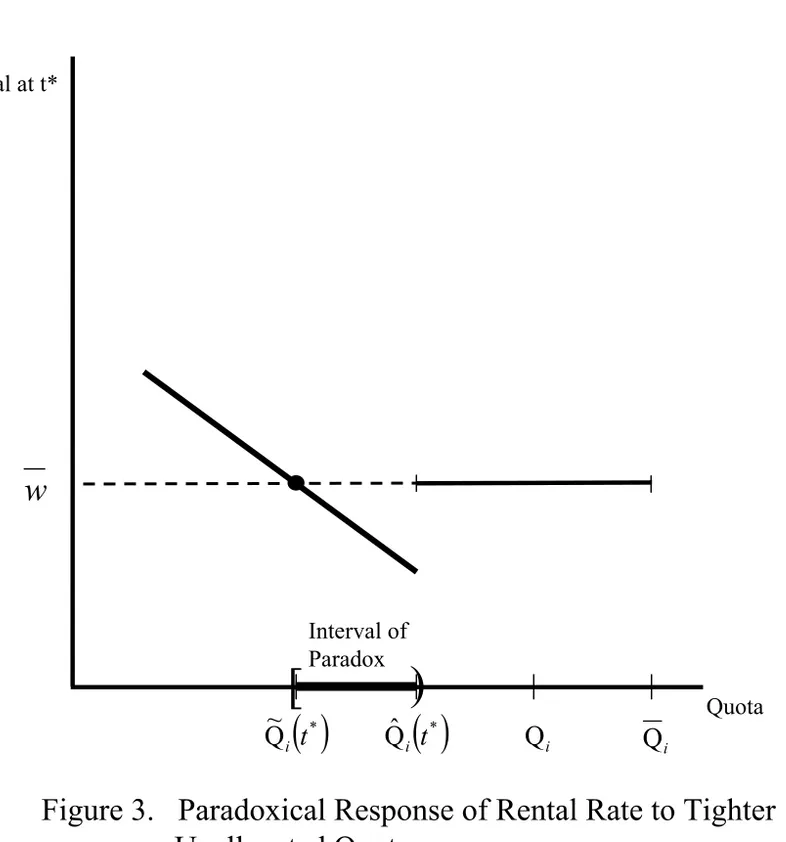
One paradoxical consequence of an anticipated tightening of the quota in any interior round merits discussion: for any date in this round before the original quota would fill, there will be an interval of tighter quotas which result in a lower, rather than a higher, rental rate. Denote the initial quota as Qi and the date when it fills as τi > θi. Choose any date in the

interval (θi, τi) and denote it t∗. Since t∗ < τi, w(t∗) = ¯w. There will exist a tighter quota,

denoted ˆQi(t∗), which would fill at exactly t∗. Given (9), ˆQi(t∗) must solve the equation

g(t∗_{, Z) = 0. This equation must have at least one solution since the function is continuous}

in its second argument, with g(t∗_{, 0) > 0 and g(t}∗_{, Q}

i) < 0. Moreover, since the function

is strictly decreasing in its second argument, the root ˆQi(t∗) is unique. As Z ↑ ˆQi(t∗),

w(t∗) _{↓ D( ¯}S + I(θi) + ˆQi(t∗)) < ¯w. The tighter quota induces a lower rental because it

induces an upward jump in the stock of imports just prior to t∗_{. Any smaller quota (Z)}

will fill before t∗_{, inducing a rental at t}∗ _{of D( ¯S + I(θ}

i) + Z, t∗). Denote this function f (Z).

Since it is continuous, with f (0) > ¯w and f ( ˆQi) < ¯w, there will be at least one solution to

the equation f (Z) = ¯w. Indeed, since f (_{·) is strictly decreasing, there must be exactly one} solution. Denote that solution ˜Qi(t∗). It follows that for any anticipated ith round quota in

( ˜Qi(t∗), ˆQi(t∗)), the rental at t∗ will be strictly smaller than when the quota is larger than

ˆ

Qi(t∗). Figure 3 illustrates this result.

[Figure 3 goes here]

8_{If a corner occurs in the i}th_{round, then p(θ}

i) > ¯p and exporters selling at that instant can earn a profit.

Exporters selling nothing at that instant, however, would have no incentive to alter their behavior provided we make either of the following assumptions: (1) there are an infinite number of firms and the probability that any one of them can fill in an instant some part (or all) of the remaining quota is zero or (2) there are an infinite number of firms but each can produce in an instant at no more than a finite rate. Under either assumption, no individual seller, even if he failed to export anything at that instant, would anticipate that his discounted wealth would increase if he tried to sell at that instant: under (1), the potential wealth gain at that instant is finite and would occur with probability zero while, under (2), the positive profit flow would be finite and would last only for an instant (a set of measure zero). The rest of the results in the paper also hold for either assumption.

3.1 Uncertainty about the Size of Future Quotas

The foregoing analysis has assumed that agents know not merely the date (θi) when each

quota round begins but the size (Qi) of each quota. In many real-world applications, however,

the size of future quotas cannot be predicted with certainty. We conclude this section, therefore, by showing how our analysis generalizes when there is uncertainty about the size of the ith _{quota resolved when θ}

i (i = 0, . . . , n) is reached. We assume that agents

are risk neutral and have common beliefs about the size of each quota summarized in an exogenous sequence of probability distributions. Denote the random size of the ith quota by Yi, its conditional distribution function by Fi(Yi|Y1, . . . , Yi−1), and its realization by Qi. We

assume the sequence _{Fi(Yi|Y1, . . . , Yi−1)}ni=0 is given.

The price at the outset of the ith _{round will now depend on the sum of the}

quo-tas realized until that point: p(θi, I(θi) + Qi). Prior to the realization of the ith quota,

the price expected to prevail at θi is EYi+1p(θi+1, I(θi+1) + Yi+1) ≡

R

Yn+1p(θi+1, I(θi+1) +

Yi+1)dFi+1(Yi+1|Y1, . . . , Yi). Since there is no quota from t = θn+1 onward, p(θn+1, I(θn+1) +

Qn+1) = ¯p. Hence, prior to θn+1, the price expected to prevail at θn+1, is given by the

terminal condition:

EYn+1p(θn+1, I(θn+1) + Yn+1) = ¯p. (13)

The following recursive equation permits calculation of the sequence of price functions:

p(θi, I(θi) + Qi) = max{¯p, Z θi+1 θi e−r(x−θi)_{D( ¯S + I(θ} i) + Qi, x)dx + e−r(θi+1−θi)_E

Yi+1p(θi+1, I(θi) + Qi+ Yi+1)} (14)

with terminal condition (13).

If i = n, the second factor in the last term of (14) is EYn+1p(θn+1, I(θn) + Qn+ Yn+1).

Substituting I(θn)+Qn= I(θn+1), into (13), we obtain EYn+1p(θn+1, I(θn)+Qn+Yn+1).

Qn). For future reference, we use this price function to compute the price expected prior to

θn to prevail at θn: EYnp(θn, I(θn) + Yn).

If i = n_{− 1, the second factor in the last term of (14) is E}Ynp(θn, I(θn−1) + Qn−1+ Yn)}.

Substituting I(θ_n−1) + Q_n−1 = I(θn), into the function just constructed above for future

reference, we obtain EYnp(θn, I(θn−1) + Qn−1+ Yn). Using this on the right-hand side of (14),

we can compute the next price function p(θ_n−1, I(θ_n−1) + Q_n−1) . . . and so on.

Proceeding in this way, we can construct the entire sequence _{p(θi, I(θi) + Qi)}n+1i=0. As

a byproduct, we have obtained the sequence of expected prices: _{EYi+1p(θi+1, I(θi) + Qi+

Yi+1)}n+1i=0. This byproduct will be useful since, under uncertainty, the date when the ith

quota fills depends on the price expected during that round to prevail at θi+1(which in turn

depends on the sum of the quotas realized through θi+1). To compute {τi(I(θi) + Qi)}ni=0,

we use the following modified complementary slackness condition:

τi− θi ≥ 0, h(τi, Qi)≥ 0, and (τi− θi)h(τi, Qi) = 0, (15)

where

h(t, Qi) = Z θi+1

t

e−r(x−t)D( ¯S +I(θi)+Qi, x)dx + e−r(θi+1−t)EYi+1p(θi+1, I(θi)+Qi+Yi+1))− ¯p.

This stochastic equilibrium shares the essential features discussed above in the certainty case. In particular, there are still rounds when the realized quota is so small that it fills instantly (the stochastic corner case) and rounds when it is sufficiently large that it fills only after a delay (the stochastic interior case). In any interior round, there are still two instants when imports occur at an infinite rate: (1) the exogenous instant when the new quota becomes available and (2) the endogenous instant when that quota fills. Moreover, the shortage induced by each quota is still most severe immediately before the arrival of the next quota.

For simplicity, we return to our assumption of certainty when discussing in the next section the alternative regime of allocated quotas.

4 Allocated Quotas

We now consider the case where foreign producers of new durables–and owners of existing durables–are forbidden to export to the home market without a license allocating them a portion of the total quota: a license valid during [θi, θi+1) is required to export against

the ith _{quota (for i = 0, . . . n) up to some preassigned individual quota. In this regime,}

the paths depicted in Figure 1 would no longer induce an equilibrium. For, given the price path, any foreign producer who owns an individual quota would wait to manufacture and export the good until after τi when he could use his license to earn a strictly positive profit

(p(t) > ¯p). Likewise, any foreign owner of an existing durable with an export license would wait until after τi to export to the home country and would rent his asset elsewhere for

¯

w in the interim. But these responses would cause excess demand for the services of the durable in the home country during the interval (θi, τi). Hence the price and rental paths

in Figure 1 no longer induce an equilibrium. When export quotas are allocated, no foreign seller need fear that others will exhaust the quota before he has exported his durable. The license guarantees him the right to export during [θi, θi+1) at a date of his choosing.

To determine the dynamic equilibrium with allocated quotas, recall that (3) must hold at all times in the home country, whether or not the durable is being imported. According to (3), home country owners of the durable can be induced to postpone selling their asset even if its price appreciates more slowly than the rate of interest because delay gives another form of compensation besides appreciation: rental income (w(t)).

If producers abroad have licenses to export, they will produce and sell at the most profitable instant. If they export over an interval of time, they must be indifferent when they produce and sell. They will be indifferent if and only if (p(θi)− ¯p)er(t−θi)= p(t)− ¯p, for t≥ θi.

Differentiating, we obtain:

˙

p(t) = r_{{p(t) − ¯}p_}. (16)

Thus, the price the producer receives likewise does not have to appreciate as fast as the rate of interest to induce him to defer exporting because delay gives another form of compensation besides appreciation: the rental income (r ¯p = ¯w) that can be obtained from renting in the rest of the world.

Equations (3) and (16) hold simultaneously if and only if w(t) = r ¯p = ¯w.9 _{That is, as long}

as the home country’s rental is driven down to the world rental rate, foreign producers will be indifferent when they manufacture and export their products. But since w(t) = D( ¯S+I(t), t), the home country rental will be driven down to ¯w if and only if the stock of imports follows the same path as under free trade, which is given in (4).

Eventually, however, cumulative exports fill the quota and further inflows are blocked. The quota fills at τi (for i = 0, . . . , n), which is uniquely defined by the following

comple-mentary slackness condition:

τi− θi ≥ 0, D( ¯S + I(θi) + Qi, τi)− ¯w ≥ 0, and (τi− θi)[D( ¯S + I(θi) + Qi, τi)− ¯w] = 0 (17)

Until the next quota arrives at θi+1, the combination of growing demand for services and

inelastic supply pushes up the rental rate. Hence, the rental rate in a policy regime where quotas are allocated is uniquely determined as follows:

w(t) =        ¯ w for t_{∈ (θ}i, τi)

D( ¯S + I(θi) + Qi, t) for t∈ (τi, θi+1).

(18)

9_{Our analysis in this section draws heavily on the work of Henderson et. al (1997), who characterize the}

competitive equilibrium in the gold market. They regard gold as an exhaustible resource which does not depreciate but can be depleted by industrial use until none remains to be mined. In our model, the durable does not disappear due to depreciation or depletion. Instead the quota on the imported durable is depleted and ultimately exhausted, after which exports must cease.

So that durables in the home country, with their enhanced rentals, do not become more attractive than other assets, their rate of appreciation must slow in accordance with (3). That is, if w(t) > ¯w = r ¯p, then ˙p = r_{{p(t) − w(t)/r} < r{p(t) − ¯}w/r_{} = r{p(t) − ¯}p_}. Given the slower appreciation, no foreign producer would regret having exhausted his export licenses prior to this second phase of round i.

Throughout this second phase, the home country rental rate continues to grow and the rate of appreciation of the price continues to fall. When p(t) = w(t)/r, the price in the home country peaks. Until the next quota arrives, the rental rises and the price falls.

After the quota arrives, however, imports resume. As discussed previously, the home country rental must remain ¯w until the new quota fills. Hence, at the exact moment θi+1,

the rental must drop precipitously from D( ¯S + I(θi) + Qi, θi+1) to ¯w. For this to happen,

the stock of imports must jump up to satisfy some or all of the “pent-up” demand. If Qi+1

is too small to satisfy all of the pent-up demand, then the i + 1st _{quota fills instantaneously}

at θi+1. Whether an interior or a corner case arises, the downward jump in the rental must

be accompanied by a kink in the path of the price of the durable in the home country: ˙

p(θ+i+1) > ˙p(θi+1− ).

The following recursive equation uniquely defines _{p(θi)}n+1i=0:

p(θi) = max{¯p, Z τi θi ¯ we−r(x−θi)_dx + Z θi+1 τi e−r(x−τi)_{D( ¯S + I(θ} i) + Qi, x)dx + e−r(θi+1−θi)p(θi+1)}. (19)

Given _{p(θi)}n+1i=0 and (18), the equilibrium price path when quotas are allocated can be

described as follows: p(t) = Z θi+1 t e −r(x−t)_{D( ¯S + I(θ} i) + Qi, x)dx + e−r(θi+1−t)p(θi+1). (20)

Moreover, since D( ¯S + I(θi) + Qi, x) = ¯w = r ¯p for x ∈ (θi, τi), (20) reduces10 to:

p(t) = (p(θi)− ¯p)er(t−θi)+ ¯p. (21)

for t_{∈ (θ}i, τi).

Figure 4 depicts the equilibrium price and rental paths when the quotas are allocated. Distinguishing variables in the allocated and unallocated cases by the superscripts “A” and “U” respectively, we conclude that τA

i > τiU unless τiA = θi. Also p(θi)− ¯p > 0 so that

whenever τi > θi producers and owners exporting into the home market earn rents.

[Figure 4 goes here]

The generalization to uncertainty in the regime with allocated quotas is straightforward and follows the same lines as that discussed in Section 3.1. As before, the price expected in round i to prevail at θi+1 replaces the price which will actually prevail then in the recursive

equation (19); however, no modification of the complementary slackness condition in (17) is necessary since no unknown future price appears in that condition. In both regimes, the introduction of uncertainty creates the possibility that the price will jump upward or downward at the start of each quota round in response to the arrival of information about the size of the quota. No jump in the price path can occur at any other time.

10_{Rewrite (20) as p(t) =}Rθi+1

t e−r(x−t)w(x)dx + e−r(θi+1−t)p(θi+1). When x∈ (θi, τi), w(x) = ¯w = r ¯p and

hence 0 =R_θt

ie

−r(x−t)_{w(x)dx + ¯p[1 − e}r(t−θi)_{]. Adding this to the rewrite of (20) proposed above and then}

5 Discussion

We have examined the competitive equilibrium induced by imposing a sequence of quotas limiting the stock of durables importable. We considered first the policy regime where any exporter could fill the quota and then the regime where the quota is allocated to a set of license holders. In both regimes, w(t) is highest just before the arrival of the next quota.

At the moment when the shortage is greatest, the rental is highest. But the price of the durable then does not reflect this shortage. In both regimes, the price of the durable then is low and falling! Indeed, in the regime of unallocated quotas, when the shortage in the protected market is most severe, the price in that market falls to the same level as elsewhere in the world where trade is unrestricted! Even in the regime of allocated quotas, the lowest price during round i may occur when the shortage is greatest. Clearly, the price of the durable is a poor indicator of the shortage induced by the quota.11

That price is a poor indicator of immediate shortage may seem counterintuitive, but the explanation is straightforward. When the shortage is greatest, the rental reflects the tight conditions. The price, on the other hand, must reflect not only the rental then but also the rentals anticipated in the future. Because the quota limits stocks imported but not their rate of change, imports can potentially flow in at an infinite rate and eliminate the shortage the moment the new quota arrives. Given our assumption of a constant rental rate and asset price, and hence a constant opportunity cost of exporting, this is in fact what occurs in equilibrium under both certainty and uncertainty, not only when quotas are unallocated but also when they are allocated. The jump in the imported stock drives down the rental rate. The price is low when the shortage is greatest because the price must also reflect the more relaxed conditions anticipated to occur in the immediate future. The price must be

11_{For a recent example where the price of a durable is used as an indicator of shortage, see Berry et. al.}

(1999). Using the price of automobiles as an indicator in their analysis of VER’s on Japanese auto exports, they conclude that the quotas at first had little effect. On the other hand, Goldberg (1995), looking at other evidence, finds otherwise.

falling when the shortage is greatest and the rentals are highest; otherwise everyone would strictly prefer to own the durable with its high “dividends” instead of other riskless assets.

Our stylized model has abstracted from many real-world considerations. Durables are not infinitely lived and do depreciate.12 _{Moreover, in the case of cars for instance, different}

models can be regarded as differentiated products with new models arriving every Fall. To complicate matters further, the quotas imposed on Japanese auto exporters during the 1980’s went into effect every Spring–in the middle of the model year. Finally, the auto industry was dominated by a few very large producers, not obvious candidates to behave like price takers.13 _{Suppose we somehow took account of all of these complications simultaneously.}

What characteristics would the pure-strategy, Markov-perfect equilibrium display?

The price of a durable at any date would still have to equal the sum of its subsequent rentals–making due allowance for discounting and depreciation. Otherwise, opportunities would exist for the myriad of actual and potential owners of the vehicles to make additional profits. More formally, let Ik(t), for k = 1, . . . , n, denote the paths of stocks of imported

durables in the play of a pure-strategy, Markov-perfect equilibrium and ¯Sk denote inelastic

domestic stocks. Assume that one particular durable of these n types, durable j, depreciates exponentially at rate δj. Let Dj(·) denote the inverse demand curve for the services of

durable j and let wj(t) denote its rental rate. Finally, let Bj denote the bequest value of

durable j at some later instant, t∗_{. We assume that the inverse demand curve and bequest}

12_{A model where the durable depreciates and producers draw down and then exhaust their fixed stock}

of licenses will resemble cases discussed in the exhaustible resource literature covering durables. See, for example, Levhari and Pindyck (1981).

13_{It is not obvious, on the other hand, that market concentration among the producers would greatly}

influence production paths. It seems to us advisable to remember Coase’s (1972) insight–subsequently formalized by Gul, Sonnenschein and Wilson (1986)–that a monopolist producing and selling a durable must compete against the countless owners of what he previously produced and may, as a result, wield no market power. In such cases, the monopolist charges competitive prices in the Markov-perfect equilibrium. Although we are not certain about the effects of producer concentration, our discussion in the text does not depend on this issue.

function depend on the entire vector of stocks. Then arbitrage will insure that: pj(t) = Z t∗ t e −(r+δj)(x−t)_w j(x)dx + e−(r+δj)(t ∗_−t) Bj(I1(t) + ¯S1, . . . , In(t) + ¯Sn) (22) where wj(x)≡ Dj(I1(x) + ¯S1, . . . , In(x) + ¯Sn, x).

For if the left-hand side of (22) were strictly smaller than the right-hand side, every small potential owner would attempt to purchase an unbounded number of durables to rent each of them out at a strict profit; and if the left-hand side were strictly larger, no one in the entire home country would be willing to own any units of the durable since selling would be strictly preferred. Even a monopolist producer would be powerless to prevent such arbitrages by owners and potential owners. Hence, (22) must hold in any equilibrium.

But as long as (22) holds, the equilibrium price path for the jth durable (pj(t)) would

have many of the features we have emphasized: no matter how stringent the quota was, there would be (in the absence of uncertainty) no jumps in the price of the durable when a new quota arrived and none when it filled; moreover the rate of appreciation in the price of the durable ( ˙pj(t)/pj(t)) would still be bounded by the sum of the interest and depreciation

rates.14 _{Finally, the price at t would reflect not merely the tightness of the market at t but}

the conditions then anticipated to prevail in the future.

6 Conclusion

The trade theory literature typically assumes that quotas restrict the flow of nondurable imports. Such a theory cannot be expected to explain the effects of quotas which instead restrict the stock increase of durable imports. Misapplying the theory in this way generates predictions difficult to square with observation. To remedy the situation, we have constructed a simplified model which we hope captures both the nature of the actual policy and of the

14_{Differentiating, we obtain: ˙p}

good which it restricts. It would be useful in future work to take account of the process by which the quota size is determined and of the depreciation of the service flow of the durable. The standard theory, based on the usual static framework, predicts that the price jumps up when the quota binds and increases as the market tightens. We have shown that this is not what should happen if the quota applies to the stock increase of a durable. In that case, there is no jump in the price when the quota fills and, as the market reaches its tightest point, the price of the durable in the protected market falls toward (and, in the unallocated case, converges to) the free-trade level. When seen through the lens of the inappropriate standard theory, this price behavior has been taken to mean that the quota is nonbinding – at exactly the time when it is rendering the market tightest. The tightening of the market is better reflected in the increasing rental rate. The rental rate begins to increase once the quota fills and continues to rise until the new one comes into effect.

Our model also predicts that at any date during which any quota in the sequence is partially filled, the stock of imports accumulated previously will coincide with the stock accumulated under free trade. Hence, although such a policy has important effects, they are confined to the temporal phasing of the imports between successive quotas.

References

Bartle, R. and D. Sherbert (1992) Introduction to Real Analysis. New York: John Wiley and Sons.

Berry, S., J. Levinsohn, and A. Pakes (June, 1999) “Voluntary Export Restraints on Auto-mobiles: Evaluating a Trade Policy,” American Economic Review, 89, 400—430.

Coase, R. (1972) “Durability and Monopoly,” Journal of Law and Economics, 15, 143—49. Flood, R. and N. Marion (1999) “Perspectives on the Recent Currency Crisis Literature,”

International Journal of Financial Economics, 4, 1—26.

Gaudet, G., M. Moreaux, and S. Salant (2002) “Private Storage of Common Property,” Journal of Environmental Economics and Management, 43, 280—302.

Goldberg, P. (1995) “Product Differentiation and Oligopoly in International Markets: The Case of the U.S. Automobile Industry.,” Econometrica, 63, 891-952.

Gul, F., H. Sonnenschein, and R. Wilson (1986) “Foundations of Dynamic Monopoly and the Coase Conjecture,” Journal of Economic Theory, , 155—90.

Henderson, D., J. Irons, S. Salant, Sebastian Thomas (1997) “Can Government Gold be Put to Better Use,” International Finance Discussion Paper 582, Federal Reserve Board. Krugman, P. (1995) “Incidents in My Career,” in The Makers of Modern Economics, ed.

Arnold Heertje. New York: Edward Elgar, www.pkarchive.org/personal/incidents.html. Krugman, P. (1979) “A Model of Balance-of-Payments Crises,” Journal of Money, Credit

and Banking, 11, 311—25.

Levhari, D. and R. Pindyck (1981) “The Pricing of Durable Exhaustible Resources,” Quar-terly Journal of Economics, 96, 365—377.

Salant, S. (1983) “The Vulnerability of Price Stabilization Schemes to Speculative Attack,” Journal of Political Economy, 91, 1—38.

Salant, S. and D. Henderson (1978) “Market Anticipations of Government Policies and the Price of Gold.,” Journal of Political Economy, 86, 627—48.

Figure 1. Price and Rental Paths with Unallocated

Quotas in the Fully Interior Case

0

θ

τ

θ

r

w

p

=

θ

τ

θ

τ

( )

t

p

( )

t

r

w

Figure 2. Time Path of Stock of Imported Durables Under Unallocated

Quotas Compared to its Time Path Under Free Trade

i

θ

τ

θ

Figure 3. Paradoxical Response of Rental Rate to Tighter

Unallocated Quotas

w

( )

Qˆ t

Q

Q

( )

Q

~

t

[

)

Figure 4. Price and Rental Paths with Allocated

Quotas in the Fully Interior Case

0

θ

τ

θ

r

w

p

=

θ

τ

θ

τ

( )

t

p

( )

t

r

w

τ

τ

τ