Vertex partition of sparse graphs

(1)

HAL Id: tel-01882331

https://tel.archives-ouvertes.fr/tel-01882331

Submitted on 26 Sep 2018

HAL is a multi-disciplinary open access

archive for the deposit and dissemination of

sci-entific research documents, whether they are

pub-lished or not. The documents may come from

teaching and research institutions in France or

L’archive ouverte pluridisciplinaire HAL, est

destinée au dépôt et à la diffusion de documents

scientifiques de niveau recherche, publiés ou non,

émanant des établissements d’enseignement et de

recherche français ou étrangers, des laboratoires

Vertex partition of sparse graphs

François Dross

To cite this version:

François Dross. Vertex partition of sparse graphs. Other [cs.OH]. Université Montpellier, 2018.

English. �NNT : 2018MONTS011�. �tel-01882331�

(2)

THÈSE POUR OBTENIR LE GRADE DE DOCTEUR

DE L’UNIVERSITE DE MONTPELLIER

En Informatique

École doctorale : Information, Structures, Systèmes

Unité de recherche LIRMM, UMR5506

Vertex partition of sparse graphs

Présentée par François DROSS

Le 27 Juin 2018

Sous la direction de Mickael Montassier

et Alexandre Pinlou

Devant le jury composé de

Durand Bruno, Professeur, Université de Montpellier Examinateur, Président du Jury Esperet Louis, Chargé de recherches HDR, CNRS, Grenoble-INP Examinateur

Montassier Mickaël, Professeur, Université de Montpellier Co-directeur Pinlou Alexandre, Professeur, Université de Montpellier Co-directeur Rautenbach Dieter, Professeur, ULM University, Allemagne Rapporteur

(3)

(4)

Remerciements

Je tiens a remercier l’ensemble des personnes m’ayant soutenu et aidé durant ma thèse. Mes premiers remerciements vont à mes directeurs de thèse, Mickael Montassier et Alexandre Pinlou, pour m’avoir soutenu, aidé, formé et supporté depuis mon stage de Master 2, et tout au long de ma thèse. Je les remercie en particulier pour les nombreuses discussions scientifiques, d’avoir lu mon manuscrit avec attention et pour les nombreuses améliorations qu’ils ont suggérées.

Je remercie Dieter Rautenbach et Eric Sopena pour avoir accepté d’être les rapporteurs de ma thèse et de lire mon manuscrit, et pour leurs commentaires constructifs qui m’ont permis de l’améliorer. Je remercie également Louis Esperet, pour être venu participer à mon jury de thèse et pour ses commentaires le jour de la soutenance, et Bruno Durand, pour avoir accepter de présider mon jury.

Je remercie également l’ensemble de l’équipe AlGCo pour m’avoir accueilli chaleureusement, et en par-ticulier Pascal Ochem, Stéphane Bessy et Daniel Gonçalves, avec qui j’ai eu l’occasion de travailler et de voyager. Je remercie également les doctorants qui ont été mes compagnons de réflexion, de discussion, de repas et de jeux au cours de ma thèse, en particulier Marthe, Florian, Julien, Jean-Florent, Lucas, Jocelyn, Swan, Guilhem, Anaël, Valentin et Tom. Merci également à Laurie et Nicolas pour leur aide logistique.

Je souhaite également remercier les membres de ma famille, notamment mon père et ma mère, ainsi que mes soeurs, Claire et Camille, pour m’avoir toujours soutenu, même dans les moments difficiles. Je remercie également Emmanuel, Clémence, Estelle et Matthieu, pour m’avoir apporté chacun un petit rayon de soleil dans ma vie.

(5)

(6)

Résumé

Dans cette thèse, nous traiterons de partitions des sommets de graphes peu denses. Pour tout k, une coloration propre de k couleurs d’un graphe est une partition des sommets du graphe en k ensembles in-dépendants. Le premier résultat de ce style fut le théorème des quatre couleurs. Il indique que tout graphe planaire admet une coloration propre d’au plus 4 couleurs.

Un sous-graphe d’un graphe G est un graphe qui contient uniquement des sommets et des arêtes de G. À noter que comme un sous-graphe de G est un graphe, il ne peut contenir une arête de G que s’il contient ses deux extrémités. Un sous-graphe induit d’un graphe G est un sous-graphe H de G qui contient toutes les arêtes de G dont les deux extrémités sont des sommets de H. Pour G un graphe et S un ensemble de sommets de G, on note G[S] le sous-graphe induit de G dont l’ensemble de sommets est S. On appelle le graphe G[S] le sous-graphe de G induit par S. Une forêt est un graphe sans cycles, et une forêt induite d’un graphe G est un sous-graphe induit de G sans cycles.

Albertson et Bermann [3] ont fait en 1979 la conjecture suivante :

Conjecture 1 (Albertson et Bermann [3]). Tout graphe planaire admet une forêt induite contenant au

moins la moitié de ses sommets.

Cette conjecture impliquerait que tout graphe planaire admet un ensemble indépendant contenant au moins le quart de ses sommets, résultat dont la seule preuve connue actuellement repose sur le théorème des quatre couleurs.

Une notion peut-être plus connue est celle de coupe-cycle de sommets (feedback vertex set). Dans un graphe G, un coupe-cycle de sommets est un ensemble de sommets qui intersectent tous les cycles de G. Notons qu’un ensemble S ⊆ V (G) est un coupe-cycle de sommets si et seulement si G[V (G) \ S] est une forêt. Par conséquent, une formulation équivalente de la conjecture 1 est que tout graphe planaire d’ordre n admet un coupe-cycle de sommets contenant au plus n

2 sommets.

Si la conjecture 1 est vraie, elle ne peut être renforcée, comme on peut le voir grâce à une union disjointe de copies de K4, le graphe complet à quatre sommets. Le meilleur résultat connu est que tout graphe

planaire a une forêt induite sur au moins deux cinquièmes de ses sommets. C’est une conséquence directe du théorème de Borodin [9] comme quoi tout graphe planaire admet une partition de ses sommets en cinq ensembles indépendants tels que toute union de deux de ces ensembles induit une forêt.

La conjecture 1 a été prouvée, et même renforcée dans des sous-classes des graphes planaires. Par exemple, Hosono [37] a montré que tout graphe planaire extérieur admet une forêt induite contenant au moins deux tiers des sommets. Il a également donné des exemples montrant que ce résultat ne peut pas être amélioré. D’autres résultats ont été dérivés de résultats sur les colorations acycliques. Fertin, Godard et Raspaud [33] ont donné de tels résultats. Ceux qui concernent les graphes peu denses sont résumés dans la table 1.

Akiyama et Watanabe [1], ainsi qu’Albertson et Haas [2] ont indépendamment proposé la conjecture suivante :

Conjecture 2 (Akiyama et Watanabe [1], Albertson et Haas [2]). Tout graphe planaire biparti admet une

forêt induite contenant au moins 5₈ de ses sommets.

Dans l’optique de prouver cette conjecture, Alon, Mubayi et Thomas [4] ont prouvé les résultats suivants :

Theorème 3 (Alon et al. [4]). Tout graphe sans triangles avec n sommets et m arêtes admet une forêt

(9)

Famille F ordre d’une plus grande forêt induite: minorant majorant Planaire 2n 5 ⌈ n 2⌉ Planaire de maille 5 ou 6 n 2 7n 10 + 2

Planaire de maille au moins 7 2n 3

5n 6 + 1

Table 1: Minorants et majorants sur l’ordre d’une plus grande forêt induite pour certaines familles F de graphes planaires [33].

Corollaire 4 (Alon et al. [4]). Tout graphe cubique (i.e. dont tous les sommets sont de degré 3), sans

triangles et avec n sommets admet une forêt induite contenant au moins 5n₈ sommets.

Corollaire 5 (Alon et al. [4]). Tout graphe planaire sans triangles et avec n sommets admet une forêt induite

contenant au moins n

2 sommets.

Cette dernière minoration a été améliorée pour n ≥ 1 par Salavatipour [49] :

Theorème 6 (Salavatipour [49]). Tout graphe planaire sans triangles, avec n sommets et m arêtes admet

une forêt induite contenant au moins 29n−6m₃₂ sommets et donc au moins 17n+24₃₂ ≈ 0.531n sommets. En nous basant sur les méthodes développées par Kowalik, Lužar et Škrekovski [43], nous améliorons le résultat précédent :

Theorème 7. Tout graphe planaire sans triangles, avec n sommets et avec m arêtes admet une forêt

induite contenant au moins max{38n−7m₄₄ , n −m

4} sommets et donc au moins 6n+7

11 ≈ 0.545n sommets.

La preuve s’appuie sur l’existence d’une série de configurations interdites dans un contre-exemple minimum, donnant des contraintes locales sur la structure d’un tel contre-exemple. Ces contraintes locales nous per-mettent d’aboutir à une contradiction, grâce à un argument de double comptage des sommets apparaissant dans les frontières de certaines faces.

Kowalik, Lužar et Škrekovski [43] ont fait la conjecture suivante et ont donné des exemples pour prouver qu’elle ne peut pas être améliorée.

Conjecture 8 (Kowalik et al. [43]). Tout graphe planaire de maille au moins 5 et avec n sommets admet

une forêt induite contenant au moins 7n

10 sommets.

Utilisant une méthode similaire à celle utilisée pour la preuve du Théorème 7, nous avons prouvé que tout graphe planaire de maille au moins 5, avec n sommets et m arêtes admet une forêt induite contenant au moins n − 5m

23 sommets et donc au moins 44n+50

69 ≈ 0.638n sommets. Ce résultat a par la suite été amélioré

indépendamment, d’une part par Shi et Xu [50] et d’autre part par Kelly et Liu [41] :

Theorème 9 (Shi et Xu [50], Kelly et Liu [41]). Tout graphe planaire connexe de maille au moins 5, avec

n sommets et m arêtes admet une forêt induite contenant au moins 8n−2m−2

7 sommets et donc au moins 2n−2

3 ≈ 0.667n sommets.

Pour les grandes mailles, nous faisons la conjecture suivante :

Conjecture 10. Pour tout entier g ≥ 3, tout graphe planaire de maille au moins g, avec n sommets et m

arêtes admet une forêt induite contenant au moins n −m

g sommets et donc au moins n − n−2

g−2 sommets.

Nous donnons un exemple montrant que cette conjecture ne peut pas être renforcée. Avec cette conjecture pour objectif, nous prouvons le théorème suivant.

(10)

Theorème 11. Pour tout entier g ≥ 3, tout graphe planaire de maille au moins g, avec n sommets

et m arêtes admet une forêt induite contenant au moins n −4m

3g sommets et donc an moins n − 4n 3g−6

sommets.

La preuve du Théorème 11 est basée sur une réduction vers les graphes 2-connexes de degré maximum au plus 3. Elle repose sur le résultat suivant :

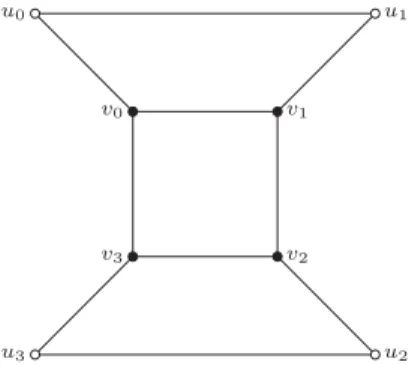
Theorème 12. Tout graphe 2-connexe de degré maximum au plus 3 avec au plus n sommets admet

une forêt induite contenant au moins 2n−2

3 sommets.

La conjecture 1 a aussi mené à des recherches similaires sur les forêts linéaires induites. Une forêt linéaire (induite) est une forêt (induite) dont le degré maximum est au plus 2. Chappell a émis la conjecture suivante (voir Pelsmajer [45]) :

Conjecture 13 (Chappell). Tout graphe planaire d’ordre n admet une forêt linéaire induite contenant au

moins 4n₉ sommets.

Cette conjecture ne peut pas être renforcée. La meilleure approche à ce jour est une conséquence du théorème suivant de Poh [47].

Theorème 14 (Poh [47]). Tout graphe planaire admet une partition en trois forêts linéaires.

Corollaire 15. Tout graphe planaire à n sommets admet une forêt linéaire induite contenant au moins n

3

sommets.

Ce problème a été résolu sur les graphes planaires extérieurs.

Theorème 16 (Pelsmajer [45]). Tout graphe planaire extérieur avec n sommets admet une forêt linéaire

induite contenant au moins 4n+2

7 sommets.

Le théorème précédent ne peut être amélioré, comme le montrent les exemples de Chappell (voir Pels-majer [45]).

Nous nous concentrons à présent sur les graphes planaires sans triangles, et faisons la conjecture suivante :

Conjecture 17. Tout graphe planaire sans triangles avec n sommets admet une forêt linéaire induite

con-tenant au moins n

2 sommets.

Nous donnons des exemples prouvant que cette conjecture ne peut pas être renforcée. Nous faisons un premier pas vers cette conjecture :

Theorème 18. Tout graphe planaire sans triangles avec n sommets et m arêtes admet une forêt linéaire

induite contenant au moins 9n−2m₁₁ sommets et donc au moins 5n+8₁₁ ≈ 0.455n sommets.

Ce théorème a une preuve du même type que celle du théorème 7. Le problème de trouver une plus grande forêt induite de degré maximum au plus d a été résolu pour tout d ≥ 2 dans les graphes de largeur arborescente (treewidth) au plus k pour tout k par Chappell et Pelsmajer [16]. À noter que le cas d = 2 correspond à la plus grande forêt linéaire induite. Ils ont également fait la conjecture suivante :

Conjecture 19 (Chappell et Pelsmajer [16]). Soit d ≥ 2 un entier. Tout graphe planaire à n sommets

admet une forêt induite de degré maximum au plus d avec au moins _4d+12dn sommets.

Pour d = 2, cela donne la conjecture 13, et pour d → ∞, cela donne la conjecture 1. Chappell et Pelsmajer ont donné des exemples montrant que cette conjecture ne peut être renforcée. À la connaissance de l’auteur, aucun progrès n’a été fait vers la conjecture 19 mis à part les cas d = 2 et d → ∞. Notons tout

(11)

de même que la minoration pour d = 2 donne indirectement des minorations pour les autres valeurs de d, donc la meilleure approche vers la conjecture 19 est le corollaire 15.

On appelle I la classe des graphes vides (i.e. sans arêtes) et F la classe des forêts. Pour tout d ∈ N, on appelle ∆d la classe des graphes de degré maximum au plus d, Fdla classe des forêts de degré maximum au

plus d, et Dd la classe des graphes d-dégénérés, c’est-à-dire des graphes dont tous les sous-graphes ont un

degré minimum d’au plus d.

Une façon de voir une forêt induite d’un graphe G est de la voir comme une partition des sommets en un ensemble induisant une forêt et un autre ensemble. Dans ce qui précède, nous avons tenté d’assurer que ce deuxième ensemble de sommets n’était pas trop grand. Une autre approche est d’imposer d’autres propriétés pour cet ensemble de sommets, par exemple qu’il induise un graphe particulier. Dans la suite, nous allons nous intéresser à cette approche.

Soient C1, C2, ..., Ckk classes de graphes. Une (C1, C2, ..., Ck)-partition d’un graphe G, notée (H1, H2, ..., Hk),

est une partition des sommets du graphe G en k ensembles H1, H2, ..., Hk tels que pour tout i ∈ {1, ..., k},

G[Hi] ∈ Ci.

L’étude des partitions des sommets des graphes planaires a commencé avec le théorème des quatre couleurs, qui peut être reformulé de la manière suivante :

Theorème 20. Tout graphe planaire admet une (I, I, I, I)-partition.

De nombreux théorèmes peuvent également être reformulés en terme de partitions en forêts. On rappelle le théorème de Poh, qui peut être reformulé comme suit :

Theorème 14 (Poh [47], reformulé). Tout graphe planaire admet une (F2, F2, F2)-partition.

De plus, une conséquence du théorème de Borodin [9] (tout graphe planaire admet une partition de ses sommets en cinq ensembles indépendants tels que toute union de deux de ces ensembles induit une forêt) est que tout graphe planaire admet une (F, F, I)-partition.

Thomassen a étudié les (Di, Dj)-partitions des graphes planaires. Il a prouvé que tout graphe planaire

admet une (F, D2)-partition [51] et une (I, D3)-partition [52] (notez que F = D1 et I = D0).

Toutefois, il y a des graphes planaires qui n’ont pas de (F, F)-partition [17], et même des graphes planaires qui n’ont pas de (F, I, I)-partition (Wegner [53]). Borodin et Glebov [11] ont montré le théorème suivant :

Theorème 21 (Borodin et Glebov [11]). Tout graphe planaire de maille au moins 5 admet une (I,

F)-partition.

Raspaud et Wang [48] ont prouvé que tout graphe planaire où deux triangles sont à une distance d’au moins 2 (et donc tout graphe planaire sans triangles) admet une (F, F)-partition.

Le résultat comme quoi tout graphe planaire sans triangle admet une (F, F)-partition est du folklore, et peut être prouvé aisément. Cependant, l’existence d’un graphe planaire sans triangles n’admettant pas de (I, F)-partition est inconnue. Nous posons les questions suivantes :

Question 22. Tout graphe planaire sans triangle admet-il une (I, F)-partition ?

Question 23. Quel est le plus petit entier d tel que tout graphe planaire sans triangles admet une (F, Fd

)-partition ?

Notons que prouver que d = 0 à la question 23 reviendrait à répondre à la question 22 par l’affirmative. On prouve le théorème suivant :

Theorème 24. Tout graphe planaire sans triangles admet une (F, F5)-partition.

Ce théorème implique que d ≤ 5 dans la question 23. La preuve du théorème précédent utilise la méthode du déchargement, avec en particulier trois configurations réductibles assez complexes. La preuve est constructive et il en découle immédiatement un algorithme en temps polynomial pour obtenir une (F, F5

(12)

Montassier et Ochem [44] donnent, pour tout d, un graphe planaire sans triangles ne pouvant pas être partitionné en deux sous-graphes induits de degré maximum au plus d, ce qui montre que la forêt dans le théorème 24 ne peut pas être remplacée par une forêt de degré borné (ou même par un sous-graphe de degré borné).

Nous montrons également que pour tout d, s’il existe un graphe planaire sans triangles qui n’admet pas de (F, Fd)-partition, alors le problème consistant à décider si un graphe planaire sans triangles donné admet

une (F, Fd)-partition est NP-complet. La preuve est une réduction vers Planar 3-Sat.

Le degré moyen maximum d’un graphe G, noté mad(G), est le maximum, sur tous les sous-graphes H de G, de deux fois le nombre d’arêtes de H sur le nombre de sommets de H. Il s’agit d’une mesure locale de la densité d’un graphe, à comprendre que si un graphe a un degré moyen maximum borné, il n’est en quelques sortes dense nulle part. La formule d’Euler nous indique que les graphes planaires ont un degré moyen maximum strictement inférieur à 6, et plus généralement, que pour tout entier g, les graphes planaires de maille au moins g ont un degré moyen maximum strictement inférieur à 2g

g−2.

Borodin et Kostochka [15] ont montré le théorème suivant :

Theorème 25 (Borodin et Kostochka [15]). Pour tout j ≥ 0 et tout k ≥ 2j + 2, tout graphe G avec

mad(G) < 212 −_(j+2)(k+1)k+2 2admet une (∆j, ∆k)-partition.

En particulier, le théorème précédent implique que tout graphe G avec mad(G) < 8

3 admet une (I, ∆2

)-partition, et que tout graphe G avec mad(G) < 14

5 admet une (I, ∆4)-partition. Avec la formule d’Euler, on

obtient le résultat suivant :

Corollaire 26. Tout graphe planaire de maille au moins 7 admet une (I, ∆4)-partition, et tout graphe

planaire de maille au moins 8 admet une (I, ∆2)-partition.

Borodin et Kostochka [14] ont montré le théorème suivant :

Theorème 27 (Borodin et Kostochka [14]). Tout graphe G avec mad(G) < 12

5 admet une (I, ∆1)-partition.

Ce dernier théorème implique que tout graphe planaire de maille au moins 12 admet une (I, ∆1)-partition,

ce qui a été amélioré par Kim, Kostochka et Zhu [42] :

Theorème 28 (Kim, Kostochka et Zhu [42]). Tout graphe G sans triangles avec mad(G) < 11₉ admet une

(I, ∆1)-partition.

Corollaire 29. Tout graphe planaire de maille au moins 11 admet une (I, ∆1)-partition.

À l’inverse, Borodin, Ivanova, Montassier, Ochem et Raspaud [13] ont exhibé, pour tout entier d, un graphe planaire de maille au moins 6 qui n’admet pas de (I, ∆d)-partition. Montassier et Ochem [44] ont

montré que cela implique que le problème de décider si un graphe de maille au moins 6 admet une (I, ∆d

)-partition est NP -complet pour tout d ≥ 1. Ils ont également prouvé que le problème de décider si un graphe de maille au moins 7 a une (I, ∆2)-partition est aussi NP-complet. Esperet, Montassier, Ochem et

Pinlou [30] ont montré que le problème de décider si un graphe planaire de maille au moins 9 admet une (I, ∆1)-partition est NP-complet.

Notons que si les théorèmes 25, 27 et 28 ne peuvent voir leurs résultats en terme de degré moyen maximum améliorés, leurs corollaires en terme de graphe planaire de grande maille le peuvent peut-être. En particulier, les questions suivantes restent ouvertes :

Question 30. Tous les graphes planaires de maille au moins 7 admettent-ils une (I, ∆3)-partition ? Question 31. Tous les graphes planaires de maille au moins 10 admettent-ils une (I, ∆1)-partition ?

Une façon naturelle d’étendre les résultats précédents est de considérer les partitions de graphes peu denses en un ensemble indépendant (i.e. induisant un graphe vide) et un ensemble induisant une forêt de degré borné, c’est-à-dire une (I, Fd)-partition. Notons que si un graphe admet une (I, Fd)-partition, alors

il admet une (I, ∆d)-partition, et qu’une (I, F1)-partition est identique à une (I, ∆1)-partition. Donc les

(13)

• pour tout entier d, il existe un graphe planaire de maille au plus 6 qui n’admet pas de (I, Fd)-partition ;

• il existe un graphe planaire de maille au plus 7 qui n’admet pas de (I, F2)-partition ;

• il existe un graphe planaire de maille au plus 9 qui n’admet pas de (I, F1)-partition ;

• tout graphe planaire de maille au moins 11 admet une (I, F1)-partition.

Nous prouvons les résultats suivants :

Theorème 32. Soit M un nombre réel tel que M < 3. Soit d ≥ 0 un entier et G un graphe tel que

mad(G) < M . Si d ≥ 2

3−M − 2, alors G admet une (I, Fd)-partition.

Theorème 33. Soit M un nombre réel tel que 8

3 ≤ M < 3. Soit d ≥ 0 un entier et G un graphe tel

que mad(G) < M . Si d ≥ 1

3−M, alors G admet une (I, Fd)-partition.

On montre les deux théorèmes précédents en appliquant la méthode du déchargement. Certaines con-figurations peuvent être arbitrairement grandes, suite à la construction d’une structure que nous appelons

forêt légère.

Par la formule d’Euler, on obtient le corollaire suivant :

Corollaire 34. Soit G un graphe planaire de maille au moins g.

1. Si g ≥ 7, alors G admet une (I, F5)-partition.

Les corollaires 34.2 et 34.3 viennent du théorème 33, alors que le corollaire 34.1 vient du théorème 32. Voir la table 2 pour un résumé des résultats sur les partitions des sommets de graphes planaires vus précédemment. Pour autant que l’on sache, les graphes planaires de maille 7, 8 et 10 respectivement pourraient tous avoir une (I, Fd)-partition pour d = 3, d = 2 et d = 1 respectivement. Cependant, observons :

Remarque 35. Pour tout entier d, il existe un graphe de degré moyen maximum strictement inférieur à

M = 3(1 −_8d1), qui n’a pas de (I, ∆d)-partition (et donc pas de (I, Fd)-partition).

Comme M = 3(1 − 1

8d) est équivalent à d = 3

8(3−M ), cela montre que le Théorème 33 peut au plus être

amélioré d’un facteur 3 8.

Un graphe est un chemin si ses sommets peuvent être notés v1, v2, ..., vn de telle manière que les arêtes

sont les vivi+1 pour i dans {1, 2, ..., n − 1}. Les sommets v1 et vn sont les extremités du chemin. Un graphe

G est connexe si pour toute paire de sommets de G, ces sommets sont les extremités d’un sous-graphe de G qui est un chemin. Dans un graphe G, les composantes connexes de G sont les sous-graphes connectés

maximaux (pour la relation de sous-graphe) de G. Pour tout entier k, on note Ok la classe des graphes dont

chaque composante connexe a au plus k sommets.

Esperet et Ochem [32] ont montré le théorème suivant :

Theorème 36 (Esperet et Ochem [32]). Tout graphe planaire de maille au moins 6 admet une (O12, O12

)-partition.

Borodin et Ivanova [12] donnent une partition pour les graphes planaires de maille au moins 7:

Theorème 37 (Borodin et Ivanova [12]). Tout graphe planaire de maille au moins 7 admet une (O3, O3

(14)

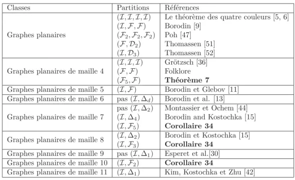
Classes Partitions Références Graphes planaires

(I, I, I, I) Le théorème des quatre couleurs [5, 6] (I, F, F) Borodin [9]

(F2, F2, F2) Poh [47]

(F, D2) Thomassen [51]

(I, D3) Thomassen [52]

Graphes planaires de maille 4

(I, I, I) Grötzsch [36]

(F, F) Folklore

(F5, F) Théorème 7

Graphes planaires de maille 5 (I, F) Borodin et Glebov [11] Graphes planaires de maille 6 pas (I, ∆d) Borodin et al. [13]

Graphes planaires de maille 7

pas (I, ∆2) Montassier et Ochem [44]

(I, ∆4) Borodin and Kostochka [15]

(I, F5) Corollaire 34

Graphes planaires de maille 8 (I, ∆2) Borodin et Kostochka [15]

(I, F3) Corollaire 34

Graphes planaires de maille 9 pas (I, ∆1) Esperet et al.[30]

Graphes planaires de maille 10 (I, F2) Corollaire 34

Graphes planaires de maille 11 (I, ∆1) Kim, Kostochka et Zhu [42]

Table 2: Quelques partitions de graphes planaires.

Notons que O2= ∆1, donc le théorème 28 peut être reformulé de la manière suivante :

Theorème 28 (Kim, Kostochka et Zhu [42], reformulé). Tout graphe sans triangles de degré moyen

maxi-mum au plus 11₉ admet une (I, O2)-partition.

Corollaire 29 (reformulé). Tout graphe planaire de maille au moins 11 admet une (I, O2)-partition.

Le théorème suivant est aussi démontré grâce à la méthode du déchagement. Là encore, certaines con-figurations peuvent être arbitrairement grandes.

Theorème 38. Tout graphe G tel que mad(G) < 5₂ admet une (I, O3)-partition.

Avec la formule d’Euler, on obtient le résultat suivant :

Corollaire 39. Tout graphe planaire de maille au moins 10 admet une (I, O3)-partition.

Comme dans les graphes planaires de maille au moins 10, il n’y a pas de triangles, le corollaire 39 implique le corollaire 34.3, c’est à dire que tout graphe planaire de maille au moins 10 admet une (I, F2)-partition.

Pour étendre notre résultat aux (I, Ok)-partitions pour d’autres valeurs de k nous prouvons le théorème

suivant.

Theorème 40. Soit k ≥ 2 un entier. Tout graphe G tel que mad(G) < 8k 3k+1 = 8 3 1 1 − 1 3k+1 2 admet une (I, Ok)-partition.

Ce dernier théorème est prouvé à l’aide de la méthode du déchargement. Certaines configurations in-terdites peuvent être arbitrairement grandes (même à k fixé), et ces configurations ainsi que la procédure de déchargement reposent sur des constructions complexes dépendant directement de (I, Ok)-partitions de

sous-graphes du graphe considéré. Il est intéressant de noter que par conséquent, la preuve ne donne pas un algorithme en temps polynomial pour construire les partitions voulues.

Par conséquent, pour k = 9, on obtient que tout graphe tel que mad(G) < 18

7 admet une (I, O9)-partition,

(15)

Corollaire 41. Tout graphe planaire de maille au moins 9 admet une (I, O9)-partition.

On peut également voir les graphes planaires de grandes mailles comme des graphes planaires avec un ensemble de cycles interdits. Il est alors naturel de chercher, pour diverses partitions, quels sont les ensembles

S de cycles tels que les graphes planaires sans cycles dans S admettent de telles partitions.

Choi, Liu et Oum [38] ont prouvé qu’il existe deux ensembles minimaux pour l’inclusion S1et S2de cycles

tels que pour i ∈ {1, 2}, tout graphe planaire sans cycles appartenant à Si admet une (I, ∆d)-partition pour

une certaine constante d.

• S1 est l’ensemble des cycles de taille impaire. Les graphes sans cycles dans S1 sont exactement les

graphes bipartis, i.e. les graphes qui admettent une (I, I)-partition.

• S2 est l’ensemble des cycles de taille 3, 4 et 6. Les graphes planaires sans cycles dans S2 admettent

une (I, ∆45)-partition.

Cela soulève la question suivante :

Question 42. Quel est le plus petit entier d tel que tout graphe planaire sans cycles dans S2 admet une

(I, ∆d)-partition.

Notons qu’interdire les sous-graphes de S2 comme sous-graphe ou comme sous-graphe induit est

équiva-lent.

On prouve le théorème suivant à l’aide de la méthode du déchargement. On utilise des classes de configurations interdites arbitrairement grandes, bien que les règles de déchargement elles-mêmes soient locales.

Theorème 43. Tout graphe sans cycles dans S2 admet une (I, ∆6)-partition.

Notons que comme les graphes planaires de maille au moins 7 sont les graphes planaires sans cycles dans

S2∪ {5}, le théorème précédent peut être comparé au Corollaire 26.

Corollaire 26 (Borodin et Kostochka [15], rappel). Tout graphe planaire de maille au moins 7 admet une

(I, ∆4)-partition, et tout graphe planaire de maille au moins 8 admet une (I, ∆2)-partition.

On prouve également le théorème suivant grâce à une réduction en temps polynomial depuis le problème de l’existence d’une (I, ∆1)-partition pour les graphes planaires de maille au moins 9 [31].

Theorème 44. Pour tout entier k ≥ 1, soit tout graphe planaire sans cycles dans S2 admet une

(I, ∆k)-partition, ou décider si un graphe planaire sans cycles dans S2 admet une (I, ∆k)-partition est

un problème NP-complet.

De plus, on construit un graphe planaire sans cycles dans S2 qui n’admet pas de (I, ∆3)-partition. Cela

implique le corollaire suivant :

Corollaire 45. Décider si un graphe planaire sans cycles dans S2admet une (I, ∆3)-partition est un

(16)

Summary

In this manuscript, we will talk about vertex partitions of sparse graphs. The study of vertex partitions of graphs originated with the Four Colour Theorem, that states that the vertex set of every planar graph can be partitioned into four sets such that no edge has both of its endpoints in one of those sets.

An induced subgraph of a graph G is a subgraph of G that is solely obtained by removing vertices (and their pendent edges) from G. An induced forest of a graph G is an induced subgraph of G that has no cycles. Albertson and Berman [3] conjectured that every planar graph has an induced forest containing at least 1

2 of its vertices. One motivation for this conjecture was that it implies that every planar graph has

an independent set on at least 1

4 of its vertices, since every acyclic graph is bipartite. That last result is a

corollary of the Four Colour Theorem, the proof of which was computer assisted, and an independent proof of that result would be appreciated.

Akiyama and Watanabe [1] on the one hand, and Albertson and Haas [2] on the other hand, independently conjectured that every bipartite planar graph has an induced forest on 5

8 of its vertices. In an attempt to

prove that conjecture, Alon, Mubayi, and Thomas [4] showed that every triangle-free planar graph admits an induced forest on at least 1

2 of its vertices. That bound was later improved by Salavatipour [49], who

showed that every triangle-free planar graph with n vertices and m edges admits an induced forest with at least 29n−6m

32 vertices, and thus at least 17n+24

32 ≈ 0.531n vertices. We show that every triangle-free planar

graph with n vertices and m edges admits an induced forest with at least 38n−7m

44 vertices, and thus at least 6n+7

11 ≈ 0.545n vertices. The proof is presented in Section 2.3. See also the arXiv version [24].

An induced linear forest in a graph is an induced forest with maximum degree at most 2. Chappell conjectured that every planar graph with n vertices admits an induced linear forest with at least 4n

9 vertices.

Poh [47] proved that the vertices of any planar graph can be partitioned into three sets inducing linear forests, and thus that every planar graph admits an induced linear forest on at least 1

3 of its vertices. On

outerplanar graphs, Pelsmajer [45] proved that every outerplanar graph with n vertices admits an induced linear forest with at least 4n+2

7 vertices, which is tight. We conjecture that every triangle-free planar graph

has an induced linear forest on at least 1

2 of its vertices, and prove that if this is true, it is tight. As a first

step, we prove that every triangle-free planar graph of order n and size m admits an induced linear forest of order at least 9n−2m

11 ≥ 5n+8

11 . The proof is presented in Section 2.4. See also the arXiv version [27].

The girth of a graph is the length of a smallest cycle in the graph. Shi and Xu [50] on the one hand, and Kelly and Liu [41] on the other hand, independently proved that every connected planar graph of girth at least 5, with n vertices and m edges has an induced forest on at least 8n−2m−2

7 vertices, and thus at least 2n−2

3 vertices. We conjecture that for all g, every planar graph with n vertices, m edges and girth at least g

admits an induced forest on at least n −m

g vertices. If that conjecture is true, it is the best possible, since a

disjoint union of k cycles of length g has kg vertices and kg edges, and its largest induced forest has k(g − 1) vertices. There is a trivial bound of n − 2m

g vertices since removing

2m

g edges is enough to get a forest. We

prove that such a graph admits an induced forest on at least n − 4m

3g, improving on known lower bounds

for g ≥ 8. The proof is presented in Sections 2.5 and 2.6. Those results were published in Discrete Applied Mathematics [25].

The presence of a large induced forest in a graph G can be seen as a partition of the vertices of G into two sets: one that induces a forest and one whose size is bounded in terms of the number of vertices of G. One can think of other conditions on the second set of vertices, for instance that it induces an other graph

(17)

with nice properties (for example a second forest). That leads us to study vertex partitions.

We denote by I the class of empty graphs, which are graphs with no edges, and by F the class of forests, which are graphs with no cycles. For all d, we denote by Fd the class of forests with maximum degree at

most d. For C0 and C1 two classes of graphs, a (C0, C1)-partition of a graph G is a partition of the vertices

of G into two sets C0 and C1, such that for i ∈ {0, 1}, the graph induced by Ci in G is in Ci.

It is easy to show that every triangle-free planar graph admits an (F, F)-partition, which corresponds to an (F, Fd)-partition where d goes to infinity. Borodin and Glebov [11] proved that every planar graph

of girth at least 5 admits an (I, F)-partition, that is an (F, F0)-partition. We raise the question for all d

whether every triangle-free planar graph admits an (F, Fd)-partition. We show that the answer is yes for

d ≥ 5, and that if the answer is no for a given d, it is NP-difficult to decide whether a triangle-free planar

graph admits an (F, Fd)-partition. The proofs are presented in Sections 3.2 and 3.3. Those results were

presented at Eurocomb 2015 and published in European Journal of Combinatorics [28].

For all d, let ∆d be the class of graphs with maximum degree at most d. The maximum average degree

of a graph is the maximum of the average degrees of its subgraphs. A lot of research has been done on (I, ∆d)-partitions of sparse graphs. Borodin and Kostochka [15] showed that every planar graph of girth at

least 7 (resp. 8) admits an (I, ∆4)-partition (resp. an (I, ∆2)-partition), and Kim, Kostochka, and Zhu [42]

proved that every planar graph of girth at least 11 admits an (I, ∆1)-partition (or, equivalently, admits an

(I, F1)-partition). We focused on (I, Fd)-partitions and showed that every planar graph of girth at least 7

(resp. 8, 10) admits an (I, Fd)-partition for d = 5 (resp. 3, 2). Our results, as well as those of Borodin and

Kostochka [15] and Kim, Kostochka, and Zhu [42] are corollaries of more general results on graphs with low maximum average degree. The proofs are presented in Sections 3.4 and 3.5. See also the arXiv version [26]. For all k, let Ok be the class of graphs whose components have at most k vertices. We prove that every

planar graph of girth at least 10 admits an (I, O3)-partition. We also show that for all k, every graph G with

maximum average degree less than 8k 3k+1 = 8 3 1 1 − 1 3k+1 2

admits an (I, Ok)-partition, implying that every

planar graph of girth at least 9 admits an (I, O9)-partition. Again, those results are corollaries of results on

graphs with low maximum average degree. The proofs are presented in Sections 4.2, 4.3, and 4.4.

The class C of (C3, C4, C6)-free planar graphs is the class of planar graphs with no subgraph (or

equiv-alently no induced subgraph) that is a cycle of size 3, 4 or 6. Choi, Liu, and Oum [38] showed that there are two minimal sets of cycles such that planar graphs with no cycles in one of those sets admit an (I, ∆d

)-partition for some d. Those sets are the set of all odd cycles on the one hand (graphs with no odd cycles are bipartite and thus have (I, ∆0)-partitions), and the set of cycles with size 3, 4, and 6 on the other

hand. They showed that graphs in C admit an (I, ∆45)-partition, and we show that such graphs have an

(I, ∆6)-partition. We also show that there exists a graph in C that has no (I, ∆3)-partition. The proofs are

presented in Sections 4.5 and 4.6. See also the arXiv version [29]. Here are references to the author’s works.

[20] K.K. Dabrowski, F. Dross, M. Johnson, and D. Paulusma. Filling the complexity gaps for colouring planar and bounded degree graphs. In International Workshop on Combinatorial Algorithms, pages 100–111. Springer, 2015.

[21] K.K. Dabrowski, F. Dross, M. Johnson, and D. Paulusma. Filling the complexity gaps for colouring planar and bounded degree graphs. arXiv1506.06564, 2015.

[22] K.K. Dabrowski, F. Dross, and D. Paulusma. Colouring diamond-free graphs. Journal of Computer

and System Sciences, 89:410–431, 2017.

[23] F. Dross. Fractional triangle decompositions in graphs with large minimum degree. SIAM Journal on

Discrete Mathematics, 30(1):36–42, 2016.

[24] F. Dross, M. Montassier, and A. Pinlou. Large induced forests in planar graphs with girth 4 or 5.

arXiv:1409.1348, 2014.

[25] F. Dross, M. Montassier, and A. Pinlou. A lower bound on the order of the largest induced forest in planar graphs with high girth. Discrete Applied Mathematics, 214:99–107, 2016.

(18)

[26] F. Dross, M. Montassier, and A. Pinlou. Partitioning sparse graphs into an independent set and a forest of bounded degree. Electronic Journal of Combinatorics, vol 25, issue 1, 2018.

[27] F. Dross, M. Montassier, and A. Pinlou. A lower bound on the order of the largest induced linear forest in triangle-free planar graphs. arXiv1705.11133, 2017.

[28] F. Dross, M. Montassier, and A. Pinlou. Partitioning a triangle-free planar graph into a forest and a forest of bounded degree. European Journal of Combinatorics, 66:81–94, 2017. Selected papers of EuroComb15.

(19)

(20)

Chapter 1

Introduction

The study of colouring of planar graphs originated in 1852 with the famed Four Colour Conjecture made by Francis Guthrie. Allegedly, he was trying to colour a map of British counties such that no two counties sharing a border have the same colour, and noticed that he needed exactly four colours. He then conjectured that this result could be generalised to any map. He posed this problem to his younger brother Frederick Guthrie, who posed it to his professor Augustus De Morgan [54].

The first proof of this result was published by Kempe in 1879, but this proof was then disproved by Heawood in 1890. The conjecture then remained unproven until 1976, when it was proven by Appel, Haken and Koch [5, 6] with the help of computer computation. This proof was based on a method introduced in 1948 by Heesch, the discharging method.

When it was proven, the Four Colour Theorem was now presented in terms of graphs, using the fact that for any planar map, taking a vertex for each region of the map, and adding an edge between two vertices if the corresponding regions share a boundary leads to a planar graph.

Theorem 1.0.1 (Appel, Haken, and Koch [5, 6]). Every planar graph admits a proper colouring with at

most four colours.

The work on the Four Colour Theorem initiated a lot of research on the colourings of graphs, especially planar graphs [40]. In this thesis, we will prove some results on those generalised colourings for sparse graphs.

1.1 Definitions and notation

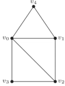
A graph G = (V, E) is a pair of sets, V and E, such that E is a set of unordered pairs of elements of V . The elements of V are called the vertices of G, and the elements of E are called the edges of G. The set of vertices of a graph G will be denoted by V (G). The set of edges of a graph G will be denoted by E(G). The

order of a graph G, denoted by |G|, is |V (G)|, and the size of a graph G, denoted by ||G||, is |E(G)|. See

Figure 1.1.1 for an illustration of a graph of order 5 and size 7.

An edge {v, w}, denoted by vw or wv, is incident to the vertices v and w, and those vertices are called the endpoints of vw. Two vertices that are incident to the same edge are adjacent. The neighbours of a

(21)

vertex v in G are the vertices that are adjacent to v. If the graph G needs to be specified, we say that a neighbour of a vertex v in G is a G-neighbour of v. For a vertex v, the set of the neighbours of v, called the

open neighbourhood of v, is denoted by N (v), and N [v] = N (v) ∪ {v} is the closed neighbourhood of v. For

all set W ⊂ V (G), N[W ] =tv∈WN [v] is the closed neighbourhood of W , and N (W ) = N [W ] \ W is the

open neighbourhood of W . For any set S of vertices, we say that any vertex in S is an S-vertex, and if a vertex in S is a neighbour of a vertex v, then we say it is an S-neighbour of v. For example, in the graph

G0 represented in Figure 1.1.1, N(v1) = {v0, v2, v4}, N [v1] = {v0, v1, v2, v4}, N ({v0, v1}) = {v2, v3, v4}, and

N [{v0, v1}] = {v0, v1, v2, v3, v4}.

v0 v1

v2

v3

v4

Figure 1.1.1: The graph G0. The circles are vertices and the lines are edges.

v0 v1 v2 v3 v0 v1 v2 v3

Figure 1.1.2: The graphs G1 (left) and G2 (right).

A graph isomorphism between two graphs G and H is a bijection f from V (G) into V (H) such that for all pair of vertices v and w in V (G), vw ∈ E(G) if and only if f(v)f(w) ∈ E(H). If there exists an isomorphism between two graphs G and H, then G and H are isomorphic. A copy of a graph G is a graph that is isomorphic to G. Generally speaking, we will work up to isomorphism, saying that two graphs are equal if they are isomorphic.

A subgraph H of a graph G is a graph such that V (H) ⊆ V (G) and E(H) ⊆ E(G). An induced subgraph

H of a graph G is a subgraph of G such that E(H) is the set of unordered pairs of vertices of H that are in E(G). For a set W ⊆ V (G) of vertices of a graph G, the subgraph of G induced by W , denoted by G[W ],

is the induced subgraph of G with vertex set W . In Figure 1.1.2, the left graph (G1) is a subgraph of G0

(Figure 1.1.1), but it is not an induced subgraph of G0. The one on the right (G2) is an induced subgraph

of G0.

Let G = (V, E) be a graph. For a set W ⊆ V , we denote by G − W the graph G[V \ W ]. For simplicity, for v ∈ V , we denote G − {v} by G − v. For a set F ⊆ E, we denote by G − F the graph (V, E \ F ). For simplicity, for e ∈ E, we denote G − {e} by G − e. For F a set of unordered pairs of elements of V such that F ∩ E = ∅, G + F = (V, E ∪ F ). For simplicity, when F is a singleton, we denote G + {e} by G + e. For example, G2= G0− v4, and G1= G2− v0v2 (see Figures 1.1.1 and 1.1.2). The action of subdividing an

edge e = vw consists in considering a vertex x /∈ V , and building the graph (V ∪ x, (E \ {e}) ∪ {vx, xw}). The degree of a vertex v is the number of edges incident to v. The degree of a vertex v in a graph G is denoted by dG(v), or simply by d(v) if there is no ambiguity on the graph G. For all d ∈ N, a d-vertex,

d+_{-vertex, or d}−_{-vertex denote a vertex with degree d, at least d, or at most d respectively. For all d ∈ N}

and all v in V , a d-neighbour, d+_{-neighbour, or d}−_{-neighbour of v denote a neighbour of v with degree d, at}

(22)

resp. minimum, of the degrees of the graph. A graph is d-regular for some integer d if all of its vertices are

d-vertices, and a 3-regular graph is called a cubic graph. For example, in G0 (Figure 1.1.1), the vertices v3

and v4are 2-vertices, the vertices v1 and v2 are 3-vertices, and the vertex v0is a 4-vertex.

Figure 1.1.3: The graphs K4 (left) and K1,3 (right)

An independent set of a graph G is a set of vertices of G that are not adjacent to one another. A clique of a graph G is a set of vertices that are pairwise adjacent. A graph whose set of vertices is independent is called an empty graph, and a graph whose set of vertices is a clique is called a complete graph. In G0

(Figure 1.1.1), the set {v0, v1, v2} is a clique, and {v1, v3} is an independent set. For all k, the complete

graph on k vertices is denoted by Kk. See Figure 1.1.3 (left) for an illustration of K4. A path of length k,

denoted by Pk+1, is the graph with k + 1 vertices {v0, v1, ..., vk} such that for i ∈ {0, ..., k − 1}, vi is adjacent

to vi+1. The cycle of length k, or k-cycle, denoted Ck, is the graph with k vertices {v0, v1, ..., vk−1} such

that for i ∈ {0, ..., k − 2}, vi is adjacent to vi+1, and such that v0 is adjacent to vk−1. A k+-cycle and a

k−_{-cycle denote a cycle of length at least k and at most k respectively. The graph G}

1(Figure 1.1.2, left) is

a 4-cycle.

A graph is bipartite if its set of vertices can be partitioned into two independent sets V1 and V2. Such

a partition into two sets is called a bipartition of the graph, and the sets V1 and V2 are called the partite

sets. A graph G is a complete bipartite graph if it has a bipartition into sets V1 and V2, such that for all

(v1, v2) ∈ V1× V2, v1v2 ∈ E(G). For all k1 and k2, the complete bipartite graph with partite sets of size

k1 and k2 is denoted by Kk1,k2. For all k, the graph K1,k is called a star. See Figure 1.1.3 (right) for an illustration of K1,3.

For two graphs G and H, a subgraph of G isomorphic to H is directly called an H of G. For example, a cycle of length three, or triangle, of a graph G is a subgraph of G isomorphic to C3. Therefore, a graph

G has no H, or is H-free, if it has no subgraph isomorphic to H. If a graph G has a cycle C on k vertices y0, y1, ..., yk−1 such that for all i ∈ {0, ..., k − 2}, yi is adjacent to yi+1 in C, and such that y0 is adjacent

to yk−1 in C, then we denote this cycle by y0y1y2...yk−1. For instance, the cycle v0v1v4 is a triangle of G0

(Figure 1.1.1). As another example, a path in a graph G is a subgraph of G isomorphic to a path. The

endvertices of a path are the vertices of degree 1 in the path.

Figure 1.1.4: The graph 2P3.

A graph G is connected if any two vertices of G are the endvertices of a path. For example, G0

(Fig-ure 1.1.1) is connected, while the graph in Fig(Fig-ure 1.1.4 is disconnected. Two vertices that are the endpoints of a path are said to be connected by this path. The distance between two vertices in a graph G is the length of a shortest path connecting these two vertices, if such a path exists. If two vertices are not connected by a path, then their distance is infinite. The distance between two vertices v and w in a graph G is denoted by

dG(v, w), or simply by d(v, w) if there is no ambiguity on the graph G. In a graph G, the components of a

(23)

such that G − S is not connected. An edge cut in a graph G is a set F ⊆ E(G) such that G − F is not connected. For all k ∈ N, a graph G is k-connected if |G| ≥ k+1 and G has no vertex cut of size at most k−1. For all k ∈ N, a graph G is k-edge-connected if it has no edge cut set of size at most k − 1. In a connected graph, a vertex v such that {v} is a vertex cut is a cutvertex, and an edge e such that {e} is an edge cut is a

bridge. In a graph G, a vertex cut S or an edge cut F separates two vertices if those vertices are in different

components of G − S or G − F respectively. For example, the graph G0 (Figure 1.1.1) is 2-connected and

2-edge-connected. The set {v0, v1} is a vertex cut that separates v2and v4, while {v0v3, v2v3} is an edge cut

that does not separate them. Note that cuts need not be minimal. For example, {v0, v1, v3} is also a vertex

cut of G0.

The disjoint union of two graphs G and H with disjoint sets of vertices is the graph (V (G)∪V (H), E(G)∪

E(H)). If the sets of vertices are not actually disjoint, we take a copy of H such that they are disjoint. We

denote by G + H the disjoint union of the graphs G and H. For G a graph and for n ∈ N, we define nG inductively by 0G = (∅, ∅), and for all n ∈ N, (n + 1)G = nG + G. See Figure 1.1.4 for an illustration of the graph 2P3.

A forest, or acyclic graph, is a graph with no cycle. A tree is a connected forest. A linear forest is a forest with maximum degree at most two. Note that the components of a linear forest are paths. The girth of a graph G is the size of a smallest cycle in G. The girth of a forest is infinite. A star forest is a P4-free forest.

In other words, it is a graph whose components are stars. The graphs K1,3 (Figure 1.1.3, right) and 2P3

(Figure 1.1.4) are forests, and even star forests. The graph 2P3is also a linear forest. For k ∈ N, a graph G

is k-degenerate if every subgraph of G has a k-vertex. Forests are exactly 1-degenerate graphs.

We denote by I the class of empty graphs and by F the class of forests. For all d ∈ N, we denote by ∆dthe class of graphs with maximum degree at most d, by Fd the class of forests with maximum degree at

most d, by Ddthe class of d-degenerate graphs, and by Odthe class of graphs whose components have order

at most d.

A colouring or vertex partition of a graph G is a partition of V (G) into several disjoint sets, which are called colour classes. A proper colouring of a graph G is a colouring of G such that every colour class is an independent set. An acyclic colouring of a graph G is a proper colouring of G such that the union of any two colour classes induces a forest.

For any classes of graphs C1, C2, ..., Cn, a (C1, C2, ..., Cn)-partition (S1, S2, ..., Sn) of a graph G is a

partition of the vertices of G into n sets S1, ..., Sn such that for all i ∈ {1, ..., n}, G[Si] ∈ Ci. For example,

({v0}, {v1, v2, v3, v4}) is an (I, F2)-partition of G0 (Figure 1.1.1). Note that an (I, I, ..., I)-partition is

exactly a proper colouring.

On further figures, we will sometimes draw only parts of some graphs, and we will use the drawing conventions described in Figure 1.1.5 for all of our figures.

vertex with all of its incident edges represented vertex with some of its incident edges not represented 3-vertex with all of its incident edges represented 3-vertex with some of its incident edges not represented 4-vertex with all of its incident edges represented 4-vertex with some of its incident edges not represented 4+

-vertex with some of its incident edges not represented Edge

Path Non-edge

Edge that may or may not be present

Figure 1.1.5: The drawing conventions for the figures.

A directed graph G = (V, A) is a pair of sets, V and A, such that A is a set of ordered pairs of elements of V . The difference with graphs is that the elements of A, called arcs, are ordered pairs, contrary to the edges of a graph. In a directed graph, the arc uv corresponds to the pair (u, v) and is different from the arc

(24)

vu. In a directed graph, an arc uv is said to go from u towards v. For all vertex v, an arc that goes from v towards another vertex is an outgoing arc of v, and one that goes towards v is an ingoing arc of v. The indegree of a vertex v, denoted d−_{(v), is the number of ingoing arcs of v, and the outdegree of a vertex v,}

denoted d+_{(v), is the number of outgoing arcs of v.}

A directed graph (V, A) is an oriented graph if for all arc uv in A, the arc vu does not belong to A. In a graph G, an orientation of G is a function which, with each edge uv of G, associates one of the corresponding ordered pairs, either (u, v) or (v, u). A graph together with an orientation yields an oriented graph. When we have a graph with an orientation, we will call the outgoing (resp. ingoing) arcs of a vertex in the corresponding oriented graph the outgoing (resp. ingoing) edges of the vertex.

A rooted tree is a tree where some specific vertex is called the root of the tree. With a rooted tree is associated a canonical orientation, where each edge is oriented from the endpoint farther from the root towards the endpoint closer to the root (in terms of distance in the graph). Such an orientation is called a bottom-up orientation. A rooted forest is a forest where every component is rooted. In a rooted forest, each vertex v that is not a root has one outgoing edge in that orientation, and the other endpoint of that edge is called the father of v. If a vertex w is the father of a vertex v, then v is a son of w.

A multigraph G = (V, E) is a pair where V is a set of vertices and E is a multiset of unordered pairs of vertices and singletons of vertices. The elements of E are still called edges, and the singletons of E are called loops.

1.2 Sparse graphs

In this thesis, we will prove properties on some classes of graphs, mainly on sparse graphs. We will use several notions of sparsity, as opposed to density, throughout this thesis. Informally, a graph is dense if it has many edges, and sparse otherwise. The average degree of a graph G, noted ad(G), is the average of the degrees of the vertices of G, that is 2||G||

|G| . One could take the average degree of a graph as a measure of its

density, but that notion does not capture the local structure of the graph. For instance, a graph composed of a clique and a large independent set has a rather low average degree, though the clique itself is dense. We will need more local notions of density, so that a subgraph of a sparse graph is sparse.

Figure 1.2.1: The graph K3,3.

A drawing or embedding of a graph G is a bijection of the set V (G) with a set of points in a surface Σ, and a bijection of the set E(G) with a set of curves in the surface Σ, such that the image of an edge vw is a curve with v and w as its extremities. A graph is planar if it can be drawn into the plane such that no two edges intersect outside of their endpoints. This drawing is a planar embedding of the graph. A plane

graph is the planar embedding of a planar graph. All the graphs represented in the figures of Section 1.1

are planar graphs, and their representations are planar embeddings. The graph K3,3 (Figure 1.2.1) is not a

planar graph.

In a plane graph, a face is a maximum connected surface that do not contain any edges and vertices. The edges and vertices that are in contact with some face φ of a plane graph G form a subgraph called the

boundary of φ and denoted by G[φ]. Two faces are adjacent if they share an edge in their boundary. The degree of a face φ, denoted by d(φ), is the number of edges that are in its boundary, counting twice the edges

that are not in the boundary of any other face. A d-face, d+_{-face, or d}−_{-face denote a face with degree d, at}

least d, or at most d respectively. In a plane graph G, let F (G) denote the set of faces of G. For example, the graph G0 (Figure 1.1.1) has four faces, bounded by the cycles v0v1v2, v0v1v4, v0v2v3, and v0v3v2v1v4.

(25)

Note that in a plane graph, any cycle corresponds to a close curve, that thus separates the plane into two parts, the interior and the exterior. If a cycle is not in the boundary of a face, then it is a separating cycle. Note that if C is a separating cycle in a graph G, then G − V (C) is disconnected. A cycle C separates two vertices if one of those two vertices is in the interior of C, and the other one is in the exterior of C. Note that if a cycle C separates two vertices, then those vertices are in different components of G − V (C), i.e.

V (C) separates those vertices.

A planar graph is outerplanar if it admits a planar embedding where every vertex is on the boundary of the same face. For example, G0(Figure 1.1.1) is outerplanar, while K4 (Figure 1.1.3, left) is not.

The dual of a plane graph G is a multigraph âG whose vertices are the faces of G and such that for all edge e of G, there is an edge between the two faces containing e in their boundaries (or the only face containing e in its boundary if there is only one such face).

For all g ∈ N with g ≥ 3, let Pg denote the class of planar graphs with girth at least g. Note that P3 is

the class of planar graphs and that P4 is the class of triangle-free planar graphs. The density of the graphs

in Pg decreases, and thus the sparsity increases, as g augments. Indeed, the larger the girth, the closer the

graph is to a tree, where the number of edges is the number of vertices minus one.

Another notion of graph density is the maximum average degree. The maximum average degree of a graph

G, denoted by mad(G), is the maximum over all subgraphs H of G of ad(H). For example, the maximum

average degree of G0 (Figure 1.1.1) is 14₅, and is equal to its average degree. The graph G0+ K1 has an

average degree of 5

2, but its maximum average degree is still 14

5 since it contains G0as a subgraph.

Those two notions are not independent. Indeed, by Euler’s formula, a connected plane graph of order

n ≥ 1, size m, and f faces verifies n − m + f = 2. Moreover, a planar graph of girth at least g has all of its

faces of degree at least g, and thus 2m ≥ fg, as every edge is either in the boundary of two faces, or counted twice in the boundary of a face. The immediate consequence is that 2m

n <

2g

g−2 for every planar graph. As

a subgraph of a planar graph is planar, we can deduce that for any planar graph G with girth at least g, mad(G) < _g2g₋₂.

Note that we can obtain the girth or the girth plus one in quadratic time thanks to a breadth first search algorithm started from each vertex, stopping when the first cycle is obtained. The girth and the maximum average degree can also be computed in polynomial time [39, 46].

1.3 Discharging method

Most of the proofs in this thesis use the discharging method. For illustration, take the proofs of Theo-rems 3.1.4, 3.1.12, 4.1.4, or 4.1.9. Cranston and West [19] give an introduction to the discharging method, as well as some applications to graph colouring. Borodin [10] gives a survey of application of the discharging method to graph colourings.

The basic principle of the discharging method is rather simple. We consider a property that we want to prove, and a class of graphs, usually sparse, on which we want to prove the property. The proof is by contradiction, thus we assume that the property does not hold on every graph of the class. We consider an order on the graphs of the class, for example the number of vertices, and we pick a smallest counter-example

G to the property in the class according to that order.

We then prove that some configurations, that we call forbidden configurations or reducible configurations, do not appear in the graph G. To prove this, first assume that the configuration appears in G. We then usually transform the graph G into a graph G′ _{that is smaller than G in the order we chose previously. As}

G is minimum according to this order, G′ _{verifies the property. Then, we prove that this implies the graph}

G also verifies the property, a contradiction.

Those forbidden configurations give us some local constraints on the structure of G. The remainder of the proof is to show that there is actually no graph in the considered class that verifies all of those constraints. This is done by first giving weight to the vertices, and sometimes to the faces of an embedding of the graph

G, such that the total weight of the graph is negative. The next step is to move the weight from some

vertices and faces to other vertices and faces, without changing the total weight of the graph, such that in the end, every vertex and every face has non-negative weight, leading to a contradiction. This part is called

(26)

the discharging procedure, and it gives its name to the discharging method.

1.4 Publications

Here is the list of publications and manuscripts of the author. First will be the works which are presented in this manuscript, and then the works that are not, but are available as an appendix.

1.4.1 Works presented in this manuscript

Large induced forests in triangle-free planar graphs

An induced forest in a graph is an induced subgraph (i.e. a subgraph obtained solely by removing vertices) with no cycles. Albertson and Berman [3] conjectured that every planar graph admits an induced forest on at least one half of its vertices. If true, that would imply that every planar graph admits an independent set on at least one fourth of its vertices, the only known proof of which relies on the Four Colour Theorem. Akiyama and Watanabe [1], and independently Albertson and Haas [2] conjectured that every bipartite planar graph admits an induced forest on at least five eights of its vertices. Salavatipour [49] proved that every triangle-free planar graph of order n and size m admits an induced forest of order at least 29n−6m

32 and

thus at least 17n+24

32 . We improve that bound by showing that a triangle-free planar graph of order n admits

an induced forest of order at least 6n+7 11 .

The proof is presented in Section 2.3. See also the arXiv version [24].

Large induced linear forests in triangle-free planar graphs

An induced linear forest in a graph is an induced forest with maximum degree at most 2. Chappell conjectured that every planar graph admits an induced linear forest on at least four ninths of its vertices. Poh [47] proved that the vertices of any planar graph can be partitioned into three sets inducing linear forests, and thus that every planar graph admits an induced linear forest on at least one third of its vertices. We conjecture that every triangle-free planar graph has an induced linear forest on at least one half of its vertices, and prove that if this is true, it is tight. As a first step, we prove that every triangle-free planar graph of order n and size m admits an induced linear forest of order at least 9n−2m

11 ≥ 5n+8

11 .

The proof is presented in Section 2.4. See also the arXiv version [27].

Large induced forests in planar graphs of large girth

The girth of a graph is the length of a smallest cycle in the graph. Shi and Xu [50], and Kelly and Liu [41] independently proved that every connected planar graph of girth at least 5, order n, and size m has an induced forest of order at least 8n−2m−2

7 , and thus at least 2n−2

3 . We conjecture that for all g, every planar

graph with n vertices, m edges, and girth at least g admits an induced forest on at least n − m

g vertices.

That would be tight if true because of the union of cycles on g vertices. There is a trivial bound of n −2m

g

vertices since removing 2m

g edges is already enough to yield a forest. We prove that such a graph admits an

induced forest on at least n −4m

3g, improving on known lower bounds for g ≥ 8.

The proof is presented in Sections 2.5 and 2.6. Those results were published in Discrete Applied Mathe-matics [25].

(F, F

d

)-partitions of triangle-free planar graphs

For all d, an (F, Fd)-partition of a graph is a partition of the vertices of the graph into two sets that are

the vertex sets of an induced forest and an induced forest of maximum degree at most d respectively. It is easy to show that every triangle-free planar graph admits a partition of its vertices into two sets that are the vertex sets of induced forests, which corresponds to an (F, Fd)-partition where d goes to infinity. Borodin