Aero – Propulsive Model Design from a Commercial Aircraft
in Climb and Cruise Regime using Performance Data
by
Magdalena TUDOR
THESIS PRESENTED TO ÉCOLE DE TECHNOLOGIE SUPÉRIEURE
IN PARTIAL FULFILLMENT FOR A MASTER’S DEGREE
WITH THESIS IN AEROSPACE ENGINEERING
M.A.Sc.
MONTREAL, JANUARY 23, 2017
ÉCOLE DE TECHNOLOGIE SUPÉRIEURE
UNIVERSITÉ DU QUÉBEC
© Copyright
Reproduction, saving or sharing of the content of this document, in whole or in part, is prohibited. A reader who wishes to print this document or save it on any medium must first obtain the author’s permission.
BOARD OF EXAMINERS
THIS THESIS HAS BEEN EVALUATED
BY THE FOLLOWING BOARD OF EXAMINERS
Ms. Ruxandra Mihaela Botez, Thesis Supervisor
Department of Automated Manufacturing Engineering at École de technologie supérieure
Mr. Thien-My Dao, Chair, Board of Examiners
Department of Mechanical Engineering at École de technologie supérieure
Mr. Guy Gauthier, Member of the jury
Department of Automated Manufacturing Engineering at École de technologie supérieure
THIS THESIS WAS PRENSENTED AND DEFENDED
IN THE PRESENCE OF A BOARD OF EXAMINERS AND THE PUBLIC ON JANUARY 19, 2017
Dedication
ACKNOWLEDGMENTS
First of all, I would to thank to Madame Ruxandra Mihaela Botez for the opportunity to study Aerospace Engineering at the ETS, and who suggested me this research topic. The work was performed at the Research Laboratory in Active Controls, Avionics and Aeroservoelasticity (LARCASE) under Dr. Botez’ supervision. Furthermore, I would like to express my sincere appreciation for her passionate mentorship, understanding and financial support throughout my Master’s program.
My great consideration and gratitude towards the LARCASE team, who encouraged me, and which has shared me, with so much patience and joy, their aerospace engineering knowledge, specifically to PhD students Ghazi Georges, Dancila Bogdan Dumitru, Dancila Radu Ioan, Murrieta-Mendoza Alejandro, Roberto S. Félix Patrón, Gabor Oliviu Sugar, and Andreea Koreanschi and to the Research Associate Mr. Oscar Carranza, for his valuable technical support.
Finally, I am grateful to my father Paul, and especially my husband Petre, for their support, the patience and great care, without which this goal would not have been achieved.
LA CONCEPTION D’UN MODÈLE AERO-PROPULSIF D’UN AVION
COMMERCIAL EN REGIMES DE MONTÉE ET EN CROISIÈRE À PARTIR DES DONNÉES DE PERFORMANCE
Magdalena TUDOR
RÉSUMÉ
Les conséquences sur l’environnement de la demande croissante dans le transport aérien, qui ont été prises en compte dans le développement de l’industrie aéronautique, ont été estimées par IATA en 2012 à 2% des émissions mondiales de dioxyde de carbone. Les acquis historiques des progrès scientifiques et techniques dans le domaine de l'aviation commerciale ont contribué à cette estimation, et même la recherche d’aujourd'hui continue de faire des progrès pour aider à réduire les émissions de gaz à effet de serre.
Les progrès, dans la conception et la technologie des modèles d'avions commerciaux et des moteurs, ont été destinés à améliorer, effectivement et efficacement, les performances de vol, mais aussi la planification de vol de ces types d'avions. Derrière ces progrès, des bases des données numériques d’un avion, qui vient d’être générées, en tant que sources de référence, la plupart du temps sont évaluées comme “confidentielles” par les constructeurs d’avions, et très rarement, elles sont traitées comme sources partagées avec ceux qui font la modélisation de l’avion et de son moteur.
La littérature de spécialité présente plusieurs modèles aéro-propulsifs d’un avion, déjà mis en œuvre, mais aucun d’entre eux n’est conçu sans avoir accès à des données numériques du moteur, en plus, il faudrait être en mesure de générer, en montée et en croisière, une base de données numériques qui peut être appliquée directement dans un processus d’optimisation des profils de vol des aéronefs.
Cette thèse a pour but d’apprendre à concevoir des modèles aéro-propulsifs pour la montée et de croisière, en utilisant des méthodes d'identification et de validation des systèmes, à travers lesquelles les performances d'avion sont calculées et stockées sous la forme la plus compacte et la plus facile d'accès à ces types de données, afin d’être utilisées dans les techniques d'optimisation du profil de vol.
Les modèles aéro-propulsifs développés dans cette recherche ont été étudiés sur deux avions appartenant à la classe d’avions commerciale. Pour chaque avion, la méthodologie a fait preuve d’une très bonne précision. Les modèles étudiés, qui prouvent avoir une bonne précision, pourraient être adaptés à d’autres avions de la même classe, même s'il n'y a pas d’accès à des données de vol du moteur. Encore plus, les résultats de la recherche ont démontré, en quelque sorte, que ces modèles pourraient économiser de l'argent pour les compagnies aériennes, par le fait qu'un très grand nombre d'essais en vol pourrait être évité,
pour chacun des cas étudiés. En outre, l’équipe du laboratoire en commande active, avionique et aéroservoélasticité (LARCASE) de l’ÉTS gagne un accès direct à ces données des performances pour ces types d’avions, dans l'intérêt de créer de nouveaux algorithmes d'optimisation applicables à d’autres types d’avions.
Mots-clés: aviation commerciale, modèles aéropropulsifs, des données numériques des
performances, méthodes d'identification et de validation du système, processus d’optimisation des profils de vol
AERO – PROPULSIVE MODEL DESIGN FROM A COMMERCIAL AIRCRAFT IN CLIMB AND CRUISE REGIME USING PERFORMANCE DATA
Magdalena TUDOR
ABSTRACT
IATA has estimated, in 2012, at about 2% of global carbon dioxide emissions, the environmental impact of the air transport, as a consequence caused by the rapidly growing of global movement demand of people and goods, and which was effectively taken into account in the development of the aviation industry. The historic achievements of scientific and technical progress in the field of commercial aviation were contributed to this estimate, and even today the research continues to make progress to help to reduce the emissions of greenhouse gases.
Advances in commercial aircraft, and its engine design technology had the aim to improve flight performance. These improvements have enhanced the global flight planning of these types of aircrafts. Almost all of these advances rely on generated performance data as reference sources, the most of which are classified as “confidential” by the aircraft manufacturers. There are very few aero-propulsive models conceived for the climb regime in the literature, but none of them was designed without access to an engine database, and/or to performance data in climb and in cruise regimes with direct applicability for flight optimization.
In this thesis, aero-propulsive models methodologies are proposed for climb and cruise regimes, using system identification and validation methods, through which airplane performance can be computed and stored in the most compact and easily accessible format for this kind of performance data. The acquiring of performance data in this format makes it possible to optimize flight profiles, used by on-board Flight Management Systems.
The aero-propulsive models developed here were investigated on two aircrafts belonging to commercial class, and both of them had offered very good accuracy. One of their advantages is that they can be adapted to any other aircraft of the same class, even if there is no access to their corresponding engine flight data. In addition, these models could save airlines a considerable amount of money, given the fact that the number of flight tests could be drastically reduced. Lastly, academia, thus the laboratory of applied research in active control, avionics and aeroservoelasticity (LARCASE) team is gaining direct access to these aircraft performance data to obtain experience in novel optimization algorithms of flight profiles.
Keywords: commercial aircraft, aero-propulsive model, aircraft performance data, climb and
cruise regimes, system identification and validation methods, flight profile optimization, flight management system
TABLE OF CONTENTS
Page
INTRODUCTION ...1
CHAPTER 1 RESEARCH PROBLEM CONTEXT ...7
1.1 General context ...7
1.2 Literature review ...8
1.3 Background ...12
1.3.1 Aero-Propulsive Model and Aircraft Performance Definitions ... 12
1.3.2 Numerical Database and Flight Management System ... 13
1.3.3 System Identification Methods ... 15
1.3.3.1 White, gray and black models ... 17
1.3.4 Estimation Methods and algorithms ... 21
1.3.4.1 Least Squares (LS) Method ... 22
1.3.4.2 Prediction-Error (PE) Method ... 24
1.3.5 Model Verification/Validation ... 25
1.3.6 Physics and Parameters of Flight ... 26
1.3.6.1 The International Standard Atmosphere (ISA) model ... 26
1.3.6.2 IAS and TAS Airspeeds, and Mach number ... 29
1.3.7 Aero-Propulsive Model Parameters ... 33
1.4 The Numerical Database Concept and Research Problem Statement ...35
CHAPTER 2 AIRCRAFT IDENTIFICATION AND METHODOLOGY ...39
2.1 Aircraft mathematical Climb Model – IAS/MACH constant ...39
2.1.1 Aerodynamics: Lift and Drag Forces Estimation ... 45
2.1.2 Propulsion: Engine Thrust and Specific Fuel Consumption Estimation ... 47
2.1.3 Estimation Methods and Algorithms ... 49
2.1.3.1 Model Identification Process ... 51
2.2 Aero-Propulsive Cruise Model ...63
2.2.1 Aerodynamics and Propulsion Estimation ... 63
2.2.2 Parameter Estimation Algorithm ... 67
2.2.2.1 Information matrix computation ... 67
2.2.2.2 The inverse of the information matrix computation ... 69
2.2.3 Cruise performance prediction ... 71
CHAPTER 3 RESULTS AND DISCUSSIONS ...73
3.1 Results and Discussions ...73
3.1.1 Validation of the Aero-Propulsive Model in Climb Phase ... 74
3.1.2 Validation of the Aero-Propulsive Model in Cruise Phase ... 85
CONCLUSION AND RECOMMENDATIONS ...99
LIST OF TABLES
Page Table 1.1 Certification source for Commercial Aviation ... 13 Table 2.1 Sample data for a commercial aircraft ... 49 Table 2.2 Inputs and Outputs Flight data of the Aircrafts A and B
in the Climb phase ... 50 Table 2.3 Inputs and Outputs Flight data of the Aircrafts A and B
in the Cruise phase ... 71 Table 3.1 Success ratios and number of flight tests in the Climb regime
for Aircraft A ... 94 Table 3.2 Success ratios and number of flight tests in the Climb regime
for Aircraft B ... 95 Table 3.3 Success ratios and number of flight tests in Cruise regime
of Aircraft A ... 96 Table 3.4 Success ratios and number of flight tests in Cruise regime
LIST OF FIGURES
Page
Figure 1.1 Static model representation ... 16
Figure 1.2 Estimation of the parameters of a mathematical model ... 18
Figure 1.3 System identification concepts ... 20
Figure 1.4 Aircraft Numerical Database and Aero - Propulsive Model (APM) Inputs and Outputs ... 36
Figure 2.1 The acting forces in the climb flight ... 40
Figure 2.2 Velocity triangle ... 43
Figure 2.3 The trajectory of an aircraft ... 52
Figure 2.4 The optimization routine ... 58
Figure 2.5 Flow chart of the model estimation process ... 60
Figure 2.6 Parameter estimation algorithm in the climb regime ... 61
Figure 2.7 3D Look-up tables representation ... 62
Figure 2.8 The acting forces in the cruise regime ... 64
Figure 2.9 Aircraft configurations in cruise flight phase ... 66
Figure 2.10 Discrete cruise trajectory of an aircraft ... 67
Figure 2.11 Parameter estimation algorithm for the cruise phase ... 70
Figure 3.1 Estimated Horizontal Distance of Aircraft A in Climb at the lowest and for three s... 76
Figure 3.2 Estimated Fuel Burn of Aircraft A in Climb at the lowest and for three s... 76
Figure 3.3 Estimated Horizontal Distance of Aircraft A in Climb at a middle and for three s ... 78
Figure 3.4 Estimated Fuel Burn of Aircraft A in Climb at a middle and for three s ... 78
Figure 3.5 Estimated Horizontal Distance of Aircraft A in Climb
at the highest and for three s ... 79 Figure 3.6 Estimated Fuel Burn of Aircraft A in Climb
at the highest and for three s ... 79 Figure 3.7 Estimated Horizontal Distance of Aircraft B in Climb
at the lowest and for three s... 81 Figure 3.8 Estimated Fuel Burn of Aircraft B in Climb
at the lowest and for three s... 81 Figure 3.9 Estimated Horizontal Distance of Aircraft B in Climb
at a middle and for three s ... 83 Figure 3.10 Estimated Fuel Burn of Aircraft B in Climb
at a middle and for three s ... 83 Figure 3.11 Estimated Horizontal Distance of Aircraft B in Climb
at the highest and for three s ... 84 Figure 3.12 Estimated Fuel Burn of Aircraft B in Climb
at the highest and for three s ... 85 Figure 3.13 Estimated Fuel Flow of Aircraft A in Cruise
at minimum and for three s ... 86 Figure 3.14 Estimated Fuel Flow of Aircraft A in Cruise
at a middle and for three s ... 87 Figure 3.15 Estimated Fuel Flow of Aircraft A in Cruise
at maximum and for three s ... 87 Figure 3.16 Estimated Fuel Flow of Aircraft A in Cruise
at minimum and for three ℎ speeds ... 88 Figure 3.17 Estimation Fuel Flow of Aircraft A in Cruise
at middle and for three ℎ speeds ... 89 Figure 3.18 Estimation Fuel Flow of Aircraft A in Cruise
at maximum and for three ℎ speeds ... 89 Figure 3.19 Estimated Fuel Flow of Aircraft B in Cruise
at minimum and for three s ... 90 Figure 3.20 Estimated Fuel Flow of Aircraft B in Cruise
XIX
Figure 3.21 Estimated Fuel Flow of Aircraft B in Cruise
at maximum and for three s ... 91 Figure 3.22 Estimated Fuel Flow of Aircraft B in Cruise
at minimum and for three ℎ speeds ... 92 Figure 3.23 Estimated Fuel Flow of Aircraft B in Cruise
at middle and for three ℎ speeds ... 93 Figure 3.24 Estimated Fuel Flow of Aircraft B in Cruise
LIST OF ABREVIATIONS
A300, A310, A320 Airbus family
ADC Air Data Computer
AE American Engineering unit system
AFM Aircraft Flight Manual
APM Aircraft Performance Model
ASCII American Standard Code for Information Interchange
AT Air Transport
ATAG Air Transport Action Group
ATC Air Traffic Control
ATM Air Traffic Management
ATS Air Transportation Systems
BADA Base of Aircraft Data
B757, B767 Boeing family
CAR Canadian Aviation Regulations
CFR Code of Federal Regulation
CO2 Carbon dioxide
CS Certification Specification
DS Dynamic System
EASA European Aviation Safety Agency
EEC Eurocontrol Experimental Center
EoM Equation of motion
FAA Federal Aviation Administration
FM Flight Manual
FMS Flight Management System
GA Genetic Algorithm
IATA International Air Transport Association ICAO International Civil Aviation Organization
ISA International Standard Atmosphere
LARCASE Laboratory of Applied Research in Active Control, Avionics
and Aeroservoelasticity
LS Least Squares
MACH Mach number
MATLAB/SIMULINK MathWorks Software product
NACA National Advisory Committee for Aeronautics
NDB Navigation Data Base
NexGen Next Generation Air Transportation System NLR National Aerospace Laboratory of the Netherlands
NM Nelder-Mead algorithm
PE Prediction Error
PDB Performance Database
PSO Particle Swarm Optimization
SA Situation Awareness level
XXIII
SAGE System for assessing Aviation’s Global Emissions
SESAR Single European Sky ATM Research
SI International System Units
TCCA Transport Canada Civil Aviation
US United States
VS Vertical Speed
LIST OF SYMBOLS AND UNITS OF MEASUREMENTS
speed of sound
input parameter of a static model
temperature variation coefficient (−0.0065°K/m or −0.0035°R/ft) acceleration factor (dimensionless)
wing aspect ratio (dimensionless) output parameter of a static model
wingspan (ft)
wing chord
csv comma separated values calibrated airspeed (KCAS)
drag coefficient (dimensionless) lift coefficient (dimensionless)
zero-lift drag coefficient (dimensionless) induced drag coefficient (dimensionless) minimum drag coefficient (dimensionless)
drag force (lbf)
Oswald efficiency coefficient (dimensionless) non-linear real-valued function
function error fuel burn (kg) FL flight level (ft)
acceleration of gravity (9.8 m/s2 or 32.174 ft/s2) gross weight (kg or lbm)
ℎ altitude (ft)
ℎ total distance traveled (nm)
horizontal distance traveled (nm or nmi) ISA international Standard Atmosphere
indicated airspeed (KIAS or nm/h)
k time index
drag due to lift factor lbf pound force
lbm pound mass
lift force (lbf)
LS least-squares model Mach number (dimensionless) matrix of independent variables MSL mean sea level
discrete value points pressure PA pressure altitude (ft)
dynamic pressure (Pa or lbm/ft3)
real gas constant (287 J/kg °K) or (1716 ft lbf/slug °R) rate of climb (ft/min)
XXVII
reference wing’s area (ft2) SLST sea-level static thrust
wing thickness
instant time
time to climb (min) temperature
thrust force (lbf)
engine specific fuel consumption coefficient (dimensionless) true air speed (KTAS or knot)
TAT total air temperature input
speed (knot)
average true airspeed (knots or kts) fuel flow (kg)
weight force (N or lbf) center of gravity position actual system’ response
model response
function of the process output ∆ standard temperature deviation (℃) Λ leading edge sweep angle (°)
pressure ratio (dimensionless) error
adiabatic constant of an ideal gas (1.4)
flight path angle
vector of parameters
temperature ratio (dimensionless)
set of minimized arguments
density (lb/ft2)
set of parameters
∗ unique solution of the equation error method
density ratio (dimensionless)
Subscript and Superscript Notations
Initial stratosphere altitude Compressible air mass
Center of gravity Flight data Distance traveled Error Altitude Leading edge Lapse rate Model
XXIX
Specific fuel consumption Static
Total Transposed
Estimated distances traveled, related to a position Fuel burnt, related to a position
INTRODUCTION
The transport of people and the goods across the globe has become a necessity and is no longer a luxury. Commercial aviation, as part of the air transportation industry, has significantly gained in popularity to meet global expectations.
In April 2014, the Air Transport Action Group (ATAG) reported that close to three billion passengers boarded an aircraft somewhere on Earth (ATAG, 2014). This global mobility has had a positive impact on the global economy, opening new international markets and facilitating the globalization of production (Budd and Goetz, 2014). However, this global mobility of goods and people has a direct negative impact on the environment. Its contribution to climate change therefore requires global action to reduce global carbon emissions.
In 2012, almost 2% of carbon dioxide (CO2) of the world’s total carbon emissions was due to airline operations (ATAG, 2014; IATA, 2013). Even if the aviation industry’s impact on the environment is relatively low compared to that of other sectors, the aerospace industry has undertaken to reduce net aviation CO2 emissions by 50%, with respect to those of 2005 by 2050, despite of increasing its activity. In 2013, IATA investigations have predicted that to reduce the air transport's carbon footprint from commercial airline fuel burn by a number of 3.2% until 2020 and of 2.9% by 2030, the air transport (AT) system have to safely improve their fuel efficiency based on the airline operational procedures (IATA, 2013). Even if the airlines are not the only contributors of this reduction process, according to the IATA' estimations, a 3.2% carbon emissions reduction could be safely accomplished with the help of an optimized air traffic management (ATM) system. Thanks to several cooperative efforts, the aircraft industry has already found some solutions to make this goal attainable.
A decade ago, studies based on flight tests for airplanes flying in formation demonstrated that a 20% reduction in airplane drag leads to an 18% savings in fuel economy, as well as a 10% reduction in carbon dioxide emissions (Okamoto, Rhee and Mourtos, 2005). Commercial
aircraft manufactures have focused on fuel efficiency since as early as 1930 (Peeters, Middel and Hoolhorts, 2005).
To improve fuel efficiency, and thereby to implicitly lower their carbon footprints, Airbus and Boeing have developed and applied advanced wing technologies on existing commercial airplanes. Airbus is a pioneer in the design of wingtip devices. These devices have been applied on the A300 and A310, reducing the spiral-shaped vortices formed during the flights at their wingtips. Airbus has continued to improve this type of research, applying large sharklets (i.e. blended winglets) wingtip devices on the 320. These have allowed to the A-320 savings up to 4% in fuel burn, as well as annual savings in CO2 emissions for each of their aircrafts (Airbus, 2015). It has been demonstrated that an aircraft equipped with winglets can climb more efficiently than an aircraft having no winglets. Also, these wingtip devices helps the aircraft to achieve cruise altitudes faster at lower thrust settings (Peeters, Middel and Hoolhorts, 2005).
The statistics are also impressive for the other giant manufacturer, Boeing. The Federal Aviation Administration (FAA) published a report in January 2015 which noted that the Boeing-737N (the Max) was going to burn 14% less fuel than the Boeing-737-800NG (FAA, 2015). According to Boeing, the Winglet Advanced Technology on the 737 MAX has optimized its wing performance, achieving a fuel efficiency of 1.8% (DTTL, 2014). On the B-747-400, the winglet design shown a 3.5% benefit in terms of cruise drag reduction (Blake, 2009).
Aerodynamic studies and their applications have been made at a reduced scale, such as an airplane’s wing and with conventional materials. The use of advanced materials on the B-787 and B-777X, such as carbon composites, have allowed improvements compared to using only conventional materials (DTTL, 2014). “Smart materials” have been used to morph the wings of an aircraft. Wing “morphing techniques” improve the aerodynamic characteristics and performance of a wing airfoil by changing its shape without using standard control surfaces. Several studies have shown that the design of a morphing aircraft wing may reduce an aircraft’s fuel consumption. An optimal (or sub-optimal) wing shape can be found for a
3
specific flight phase including take-off, climb, cruise, and descent (Gabor, Koreanschi and Botez, 2012; 2013; Gabor et al., 2014).
To achieve the fuel reduction goal by 2050, also, the engine manufacturers must improve engine efficiency. In September 2014, Airbus evaluated the latest generation of power plants: PurePower PW1100G-JM from Pratt & Whitney and CFM International’s LEAP-1A, on the A320NEO “New Engine Option” of the Airbus A320 family. According to Airbus, the A320’s improvements have resulted in significant predictions such as 15% in fuel savings per aircraft, and by 2020, 20% fuel burn improvement per seat (Airbus, 2014).
Another way to reduce CO2 emissions in aviation is the development of sustainable alternative fuels. One alternative to safely replace conventional kerosene jet fuel is to use “biofuel”. After an impressive number of tests, three different types of biofuel were approved in June 2014. Even though the high cost of biofuel was a barrier, 21 airlines used alternative fuels for commercial flights in 2014 (IATA, 2014).
As mentioned in the ICAO 2010 Environmental Report, the design and manufacturing of an aircraft can take more than 10 years (ICAO, 2010). Implementing technological improvements into a fleet in service is a long and costly process. The airspace industry is therefore working in collaboration with academia to find alternative solutions, such as new aircraft trajectory optimizations methodologies for fuel cost reduction (Murrieta Mendoza, 2013; Mendoza and Botez, 2014; Patron, Botez and Labour, 2013; Murrieta-Mendoza and Botez, 2014a; Murrieta-Mendoza and Botez, 2014b; Patrón and Botez, 2014; Patrón et al., 2013a; Patrón et al., 2013b ; Patrón, Berrou and Botez, 2014 ; Dancila, Botez and Labour, 2012). According to Jensen (Jensen et al., 2014; Jensen et al., 2013), most aircraft in the United States do not fly at their optimal trajectories in terms of altitudes and speeds. Therefore, to reduce fuel consumption, an optimization of the vertical profile would be a value-added, low-cost option (Patron, Botez and Labour, 2012; Patron, Botez and Labour, 2013; Patrón et al., 2013; Dancila, Botez and Labour, 2012). Vertical flight profile trajectory optimization is considered as the pivotal function of the Flight Management System (FMS) due to its capacity for flight cost reduction (Sibin, Guixian and Junwei, 2010).
The FMS, as an airborne electronic device employed in most commercial aircraft manages each flight, computes the optimal flight profiles (i.e. the vertical and lateral profiles) to minimize the flight costs in terms of flight time, and also the total fuel burnt (Botez, 2006). To predict the optimal flight trajectory, the FMS needs an Aircraft Performance Model (APM) that estimates the horizontal distance traveled and the amount of fuel burnt (Murrieta-Mendoza and Botez, 2014; Murrieta-(Murrieta-Mendoza, Botez and Ford, 2014; Dancila, Botez and Labour, 2013; Dancila, Botez and Ford, 2013). Predicting the optimal flight trajectory also requires the input data of an associated aircraft performance model, along with the operational instructions corresponding to its trajectory as well as the weather data. This proves how important is to have a well investigated and advanced FMS, which rely otherwise on the most reliable aircraft performance model (Sibin, Guixian and Junwei, 2010).
The behaviour of an aircraft in the classical way is described by a set of non-linear equations, called Equation of Motion (EoM), as proposed by Ghazi, G. (Ghazi, 2014) or by Vincent et al. (Vincent et al., 2012). As any electronic device, the FMS has a limited processing capacity. A simplified physical model must firstly be defined by a set of equations of motion, whose solutions are usually numerical. These solutions are then stored in so called the numerical database or look-up tables, easily adapted to the FMS architecture.
The objective of this thesis is to provide a complete methodology to conceive an Aircraft Performance Model (APM) from flight tests in climb and cruise regimes by creating look-up tables from aero-propulsive models. These aero-propulsive models were designed to meet the need of the Laboratory of Applied Research in Active Control, Avionics and Aero-Servo-Elasticity (LARCASE) team, of FMS manufacturers (CMC Electronics Esterline) and of the aircraft manufactures.
The obtained performance data by applying these proposed aero-propulsive models can be used by researchers to create algorithms and or simulations for the flight trajectory optimization in the vertical plane, in the climb and cruise phases (Murrieta-Mendoza, Botez and Ford, 2014; Dancila, Botez and Labour, 2013; Dancila, Botez and Ford, 2013). These
5
models in climb and cruise regimes were created using the numerical database of a commercial aircraft. In the climb as well as cruise flight phase, the aircraft performance for the flight tests involves a combination of aircraft aerodynamics and engine attributes (i.e. parameters).
It should be emphasized that the aircraft manufacturers are looking for the methodology that creates a numerical database using the measured flight parameters, and with a high reliability for a minimum number of flight tests (US, 1993). With these measurements collected from flight tests and stored in aircraft performance charts and tables, manufacturers can fulfill the aircraft specification compliances and utilities for a particular aircraft. Practice has revealed that the aircraft engines are not adequately equipped to collect the in-flight measurements (US, 1993). These measurements of the engine thrust are very important, as they are used to build an engine model, as part of the aero-propulsive model of any aircraft. Therefore, to create a complete aero-propulsive model, an aerodynamic model has to be developed. The aerodynamic model is also based on the measurements of the flight tests. Even with a minimum amount of information, i.e. the unknown engine performance data, this thesis proposes a complete methodology for identifying an Aero-Propulsive Model (APM) in climb and cruise regimes using numerical database of an Aircraft A. In a vertical plane (i.e. a plane perpendicular to the ground) the climb and the cruise regimes represent two essential segments of the commercial and military airplane flight profiles (Hull, 2007). The aircraft manufacturers goal is to build a reliable aero-propulsive model with a minimum access to aircraft information, and to a minimum number of flight tests. The proposed methodology to build these aero-propulsive models in the climb and cruise phases has showed a good prediction also for another numerical database of an Aircraft B belonging to the same aircraft commercial class.
This thesis shows how to create flight numerical database, without any prior engine information, in climb and cruise regimes, with a minimum flight tests number while retaining a good level of accuracy. Comparing to the existing methodologies, the new proposed methodology is therefore less costly (more economical) in terms of time and money (i.e. based on the number of the flight tests saved) for a commercial aircraft manufacturer.
This thesis research is structured on three large chapters. A literature review and a summary of the theoretical concepts are presented in Chapter 1, followed by the proposed methodology and the research problem statement under its assumptions in Chapter 2. Once the objectives, limitations and the methodology have been described, the results and discussions are analyzed in details in Chapter 3. Finally, the conclusions followed by recommendations summarize the contribution of this research topic in the aerospace field.
This research work was realized in collaboration with and was sponsored by CMC Electronics Esterline, partner of the LARCASE. The main objective was to create an aircraft performance model, in the climb and cruise regimes, using numerical database of a commercial aircraft as reference source.
CHAPTER 1
RESEARCH PROBLEM CONTEXT
This chapter defines the main terms of the research topic, including the definitions, concepts, theories and methods utilized for modeling an airplane in the climb and cruise regimes. This chapter includes a detailed description of the research problem, along with the assumptions made to orient the approach. A thorough review of the literature related to this topic is incorporated throughout.
1.1 General context
Governments and the airspace industry are looking for new strategies to achieve air transportation savings in the best interest of the planet. To constraint, and thus to reduce worldwide aviation emissions, Europe and the United States (US) have worked together in the creating and interoperating these systems: Single European Sky ATM Research (SESAR) and Next Generation Air Transportation System (NexGen) latest (Murrieta-Mendoza et al., 2015). The cooperation between Flight Management Systems (FMSs) and Air Traffic Management (ATMs) systems is possible made by use of navigation algorithms, utilized as simulation tools, and wherein future ATMs could generate modifications in flight plans to keep them (i.e. the flight plan) active (Flathers III, Allerton and Spence, 2010). Aviation applications have continually been designed to allow safe aircraft’ separation and to improve the communication infrastructure among airliners, aircraft pilots, and Air Traffic Controllers (Murrieta-Mendoza et al., 2015; Theunissen, Rademaker and Lambregts, 2011).
The new aircraft/engine technologies and operational procedures also reflect the industries objective to reduce both fuel consumption and the emissions of carbon dioxide (CO2), carbon monoxide (CO), hydrocarbons (HC), nitrogen oxides (NOx), and sulphur oxides (SOx), computed as (SO2).
To measure the efficiency of reducing global fuel burn and its environmental impact, the US Federal Aviation Administration (FAA) has developed simulation aircraft and engine models
at local/regional (dependent on weather) and at global levels (Fleming et al., 2006). The engine model has the particularity that it is assigned by default as being among the most popular ones of the airline fleet. Called the System for assessing Aviation’s Global Emissions (SAGE), this high fidelity computer model is helping the international aviation community to estimate aircraft fuel burn and emissions, as well as to make available databases and methodologies (Fleming et al., 2006). SAGE has also the ability to model variations in the parameters, as well as flight trajectories, aircraft performance (such as fuel flow) and aircraft motion data (as the operations database at the individual flight level), etc.
Optimization techniques have been studied for flight trajectories in the Aviation Industry, especially via the required criteria of minimum flight time and/or fuel consumption. These techniques, implemented on a number of FMS generations, have allowed flight crew to achieve the desired trade-off between time and fuel costs. National and international aeronautical organisation policy makers have imposed ambitious goals, such as safety improvements, increased FMS efficiency, and, last but not least, environmental sustainability.
In other words, to plan and to control the air traffic flow, in order to predict optimal flight trajectories, the ATC/ATM applications, as decision support tools, are using the most accurate Aero-Propulsive Models (APM(s)). Additionally, at that precise information on the main flight phases of a predictable flight, an APM can be employed to estimate the aircraft numerical databases, in order to obtain the exact trajectories estimates. However, the literature has few notable researches on the subject of APMs used for flight trajectory estimation.
1.2 Literature review
Sibin et al. in (Sibin, Guixian and Junwei, 2010) created a method to build an Aircraft Performance Model (APM) for FMS by using the performance data of a flight simulator prototype. As reported by Sibin’ team, the data structure requirements of the performance
9
database from their FMS flight simulator were dependent on the Object-oriented Technique, and the aerodynamic model. Meanwhile, their engine performance data has been known, as it was provided by the flight simulator prototype system. Most aircraft manufacturers hesitate to provide the aero-propulsive data to researchers, making access to aircraft performance data quite difficult. However, this research thesis comes out with the novelty through that an Aero Propulsive Model (APM) can be created without any access to engine performance data.
Two years later, Sibin et al. in (Sibin, Li and Han, 2012), proved that their Particle Swarm Optimization (PSO) algorithm improved the trajectory optimization of the Boeing 737-800 aircraft in its vertical flight profile. Their work relied on the mass point and rigid body dynamics theory (Lu, 2007; Sibin, Li and Han, 2012). This approach is used in trajectory optimization process in order to reduce the complexity of aircraft behaviour and to enhance the real-time system performance in the online computation for FMS system. Accordingly to the same authors (Sibin, Li and Han, 2012), there are other Aircraft Performance Models (APMs) constructed by Peng, under non-real-time circumstances in (Junyi and Rongzhen, 1997), and by Wang in (Wang and Yang, 2008), both accordingly to the Aircraft Flight Manual (FM).
Another Aircraft Performance Model (APM), called also Base of Aircraft DAta (BADA) is developed and maintained by Eurocontrol in collaboration with the aircraft manufacturers and operating airlines. It contains the aircraft model specifications and the datasets, and is created for needs in aircraft trajectory simulations, and for their predictions using air traffic modelling and simulations tools.
Camilleri et al. (Camilleri et al., 2012) described the structure and the main features of an APM, developed to model the Airbus A320 performance in climb, cruise and descent regimes, over its entire operational flight envelope. They used the BADA information to validate their APM.
Gong and Chan in (Gong and Chan, 2002) presented a technique to obtain an Aero-Propulsive Model (APM) from the available time-to-climb data, which can be found in any flight manual (pilot’s manual or operations manual). They performed two case studies, one study on a Boeing 737-400 for which the time-to-climb and the aero-propulsive data were known, and the other study on a Learjet 60. Boeing’s INFLT, as part of a NASA aircraft performance software package from a cooperative research project with Boeing, computed the aircraft performance of most Boeing aircraft types. The engine thrust force estimated from an available engine model helped them to build the propulsive model. This engine model was scaled so that it could optimize the trajectory predictions for a Learjet 60. Good results were obtained when the predicted trajectories were compared to those obtained from radar tracking. However, their methodology did not take into account the engine fuel consumption or the fuel burnt, and therefore their APM could not be used to solve the current optimization trajectory problems.
Baklacioglu and Cavcar in (Baklacioglu and Cavcar, 2014) applied a genetic algorithm (GA) to obtain an aero-propulsive model (APM) from the flight manual data (Boeing 737-400 Operations Manual) of a transport aircraft in order to determine the climb and descent trajectories. But, contrary to Gong and Chan (Gong and Chan, 2002), their propulsive model was based on a semi-empirical equation. Their work involved an identification process to establish the model coefficients for a Pratt & Whitney JT9D-7A engine at different altitudes and Mach numbers. The predicted time to climb resulted from the obtained model was compared with the predicted from the flight manual data.
Eight years after Gong and Chan’s research, Vallone and Mcdonald in (Vallone, 2010; Vallone and McDonald, 2010) analysed the supersonic light fighter, the Northrop F-5, and the McDonnell Douglas DC-10, a three-engine jet performances. The information was gathered from the Aircraft Flight Manuals (AFM), the Standard Aircraft Characteristics (SAC) charts, and the Jane’s All the World’s Aircraft or even the Wikipedia website.
According to the authors, the drag polar and engine deck models for these airplanes were created based on known aircraft data, using the inverse problem process. Based on the
11
engines’ characteristics, Vallone (Vallone, 2010) built some functions for the fitting of the drag polar and the engine deck (engine model) for the Northrop F-5 and the McDonnell Douglas DC-10.
Ghazi et al. in (Ghazi, Botez and Tudor, 2015) developed a methodology to design an aero-propulsive model (APM) from flight tests, and built a performance database (PDB) to predict the Cessna Citation X performance in the climb regime. A total of 70 flight tests were performed at the Research Laboratory in Active Controls, Avionics and Aeroservoelasticity (LARCASE) on a Research Aircraft Flight Simulator (RAFS) for the Cessna Citation X business aircraft. This is a level D aircraft research flight simulator, manufactured and designed by CAE Inc., for which 9 of the 70 flight tests were used in the model identification process, and the rest (61) of flight tests were used for the model validation process. The estimations of the model based on this methodology had a 100% success rate for both flight tests categories used for model identification and validation. The aero-propulsive model and the interpolation methods used by Ghazi et al. to create the PDB were sufficiently accurate (maximum deviation of less than 5%) and could be further adapted for their use on other aircrafts.
The originality of this research thesis comes from the fact that an aero-propulsive model was set up, with no a priori propulsion model information. In previous studies, Gong (Gong and Chan, 2002), and Vallone (Vallone, 2010; Vallone and McDonald, 2010) had a priori propulsive model information available, which helped them to build their aero-propulsive models. Additionally, the new proposed methodology of this accurate aero-propulsive model studied in climb and cruise regimes, was created based only on the physical approach of the problem, and it was developed based on a minimum amount of flight test data required for the identification process.
1.3 Background
1.3.1 Aero-Propulsive Model and Aircraft Performance Definitions
An aircraft Aero-Propulsive Model is described with the help of two mathematical sub-models. The first sub-model, called “aerodynamic model” is based on aerodynamic analysis, using the computation of aerodynamic forces (lift and drag) that are specific for each of the two configurations (climb and cruise) analyzed. The second sub-model, called “propulsive model” is related to the propulsion (power plant, propeller or engine), and estimates the driving thrust force and the engine performance.
This “aero-propulsion model” is designed to improve the aircraft performance. Aircraft performance is characterized by the way in which an airplane performs under a specified set of conditions in order to achieve its intended purpose of flying from point A to point B. An airplane’s performance is measured by use of:
• The physics of flight;
• The lift, drag, and thrust coefficients; • Estimation methods;
• Performance Data such as PDB, lookup tables, and flight test data for experimental data representation.
An aircraft is a market product; therefore, it has to meet performance standards fixed by laws. Gudmundsson (Gudmundsson, 2013)) and Maris (Maris and Vandevivere, 2014) presented information on commercial aviation laws, as controlled in the USA, in Europe and in Canada, according to the different rules summarized in Table 1.1.
13
Table 1.1 Certification source for Commercial Aviation
Rules USA 14 CFR Part 25 Europe CS-25 (EASA)
Canada CARs, Part V (Part 525),
TCCA (Part 521)
The progress in the design and technology of aircraft models and in ATM-FMS systems has strengthened the role of ATC services. The ATM en-route system submits the pre-planned aircraft trajectories estimated by Flight Management Systems (FMSs) to other airplanes, and to the ground ATM processors (Suchkov, Swierstra and Nuic, 2003). In (Suchkov, Swierstra and Nuic, 2003), Suchkov mentioned that one of the problems that the ATC service faces today is that not all airplanes are equipped with onboard FMSs, even if all FMSs have the ability to plan efficiently flight profiles.
An Aero-Propulsive Model (APM) was built to meet the need to optimize aircraft vertical profiles, mainly used by FMSs, in order to find the most economic flight paths in terms of time or fuel consumption.
1.3.2 Numerical Database and Flight Management System
The FMS is the key with which to responds to most of the airlines’ economic worries in terms of fuel and time costs (Creedon, 1983). In 1982, Boeing began to install FMSs on B-757 and B-767 as standard equipment, and later Airbus installed FMSs on the A310. These FMSs became standard for most commercial airplanes: the Airbus A300-600, A320, A321, A330, A340, Boeing 737-300/400/500, B747-400, and B-777, the Fokker100, and the McDonnell Douglas MD-11 and MD-90) (Liden, 1995).
The industry was not prepared for this “revolutionary advance in the management of the flight” as mentioned by Liden in his paper (Liden, 1995). Therefore, in order to meet the aircraft manufacturers’ and the airlines’ requirements, different FMS versions were designed, and during the ensuing years, new features and improvements have been added in the FMS architecture. Customers’ requirements have been met thanks to the flexibility and functionality of the FMSs’ software architecture. Due to the anticipated air traffic growth, and to the FMSs inclusion in the ATM systems, an upgrading to hardware technology should give better ratings to FMS’s market (Liden, 1995).
The airlines and the airplane manufacturers have decided to use FMSs as a long-term solution for automatized flight planning, and recording flight procedures. The computerization of the FMS has revealed remarkable advances, including pilot workload reduction, increased flight safety, the insertion of large route databases, and trajectory optimization tools (Igor and Atkins, 2001). As a very complex avionics system, an FMS has the capability to predict and optimize the flight plan based on the following parameters: weight or gross weight, aircraft type, engine and performance characteristics, winds, air temperature, etc. Other parameters include the airspeeds, Mach numbers, and altitudes needed to produce four-dimensional (4D) flight profiles (lateral and vertical), as explained by Collinson and Walter (Collinson, 2011; Walter, 2001).
The FMS architecture includes functions for navigation, flight planning, trajectory prediction, performance computations, and guidance (Walter, 2001). These functions are supported by the Navigation Data Base (NDB), and the performance database (PDB) of the airplane. The NDB must be updated monthly, while the PDB should be updated whenever a change in an aircraft’s performance characteristics occurs (e.g. an engine retrofit). The PDB encloses aircraft/engine model performance data, which is composed of the drag, thrust, fuel burnt or fuel flow (depending on the flight regime), and the speed/altitude of aircraft flight envelope. The flight envelope is defined by Shin in (Shin et al., 2011) as the safe flying area of an aircraft, as described by certain variables.
15
A vertical flight profile, calculated along a lateral path, is composed by the 3 regimes of climb, cruise and descent.
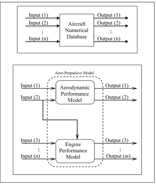
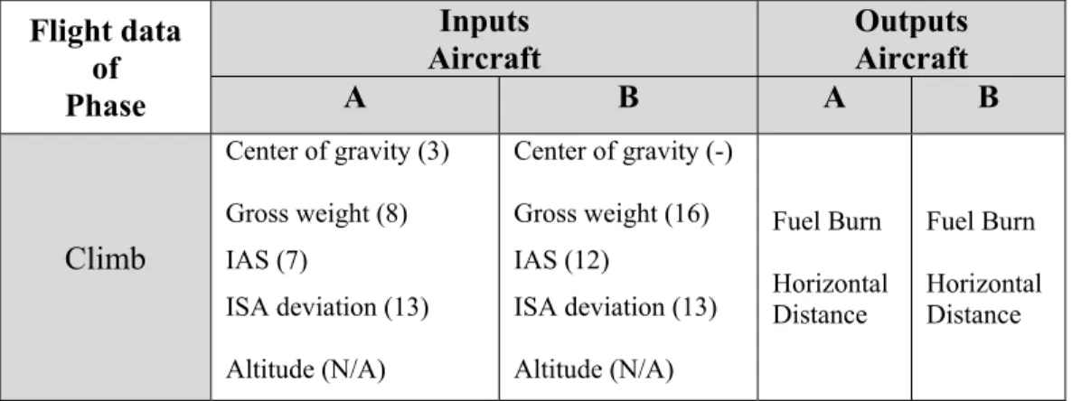
Trajectory optimization problems usually have the following inputs: the center of gravity position ( ), the speed ( ), the weight ( ) or gross weight ( ), the ISA (International Standard Atmosphere) temperature deviation (∆ ), the altitude (ℎ). The output parameters of these problems are expressed in terms of the fuel burn ( ), the horizontal distance travelled ( ) or ( ) for the climb regime, and the fuel flow ( ) for the cruise regime.
1.3.3 System Identification Methods
The behaviour of an aircraft, defined as a Dynamic System (DS), is the main concern of aeronautical engineers. They have to choose, from many features, those that are necessary and sufficient to accurately describe the DS’ objectives (Bosch and Klauw, 1994). The art of modeling firstly requires a thorough understanding of the basic problem in the real world by means of a “model”. For this reason, the real dynamic system behaviour is described by functions that are mathematical representations of the system properties.
Aerospace literature reveals a range of approaches to achieve adequate models. Bosch and Klauw (Bosch and Klauw, 1994) emphasize that a model can be developed by considering prior knowledge of the process. For example, a mass is assumed to be a point mass, without a physical size. More, prior understanding of the process can enrich the structure of a model with supplementary information. The identification techniques are further introduced. These techniques help to find approximated values for the model parameters, dependent on to the inputs and the outputs of experimental observations and measurements.
The following classification system supports a means to choosing a mathematical model to describe an aircraft as a dynamic system. Bosch and Klauw classified the models to describe a dynamical system as follows (Bosch and Klauw, 1994):
• “Mathematical models” used to study the dynamics of a system with the aid of non-linear differential equations, and assumed to be very flexible;
• “Scale models” for situations where mathematical models are not accurate enough or cannot be computed fast enough; these models are created by examining a physical process or system, and then building it on a reduced scale in order to survey their loads during wind tunnel tests at lower cost;
• “Verbal models”, with examples in sociology and psychology, in which a system is too difficult to be mathematically modeled. There must be some understanding of the qualitative relations between the system variables.
Once we understand that a mathematical model can be applied to determine an aircraft’s motions through the air, then, according to the same authors (Bosch and Klauw, 1994), the mathematical models may be subdivided into:
• “Static or steady state model” that describes the relationship between the input and the output of a function, which can be linear or nonlinear. A static model with the output , parameters and of the function, and the input is depicted in Figure 1.1.
Figure 1.1 Static model representation
This type of model is described as a time independent computing system, and whose forces are balanced. It is also a means to view an airplane as a system, for example: an aircraft that is not intended to fly is called “static model”, and is also known as an aircraft used for the testing and/or development of new designs.
a, b
17
• “Dynamic models”, which are mostly based on simulations, designed to understand the behaviours of a system by means of analysis. Typically, they are represented by differential equations, or presented as stochastic or matrix models such as black models or other such complex models.
Both the static and the dynamic models described above are “deterministic” models. These deterministic models are all those in which the output parameters are accurately determined. The aircraft may thus be designed using static and dynamic models.
The research problem analysis about the mathematical models of an airplane is continuing to be explored by means of the definitions regarding to the inputs and outputs of their parameters, and to investigate the most appropriate way to achieve their best approximation.
1.3.3.1 White, gray and black models
Starting from some basic physical laws and known parameters, we can create what is known as a ”white-box” model, that is a theoretical model. Therefore, this model could be described by some sets of equations. Under other circumstances, with no prior information, the model has to be developed from the measured data, and because lacking information about the system internal structure and its internal relations, the model is known as an empirical ”opaque” (black-box) model.
Our aero-propulsive model (i.e. an aircraft modeled after a DS concept) is a combination between these two models, and is known as a “grey” model or a “hybridization” of the above two models. Representative of a semi-empirical model class, the aero-propulsive model has unknown parameters which are computed from the experimental data, and they are also based on the theoretical (i.e. the numerical database) model built.
Mathematical modeling by means of parameter estimation is one of the techniques needed to determine a system’ characteristics (i.e. the aircraft performance parameters determined from aerodynamics and propulsion data).
Aircraft parameter estimation is the most well-known example of system identification methodology, which helps to solve the engineering inverse problem of model determination and validation through a set of observations (i.e. the flight tests data) (Hamel and Jategaonkar, 1996). Hamel et al. (Hamel and Jategaonkar, 1996) also state that the system identification methods had become the most appropriate base for model validation in research and industry, by managing aircraft design and by improving risk and cost reduction in the ideal implementation of both existing and new-generation aircrafts.
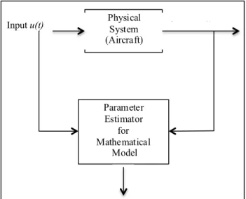
Parameter estimation is a method of using observations from a dynamic system (DS) (i.e., any aircraft as a physical system) to develop a mathematical model that represents the system’ features to an acceptable degree. This is a process of determining the unknown parameters of a mathematical model based on input–output data (flight data), and can be expressed graphically, as shown in Figure 1.2.
Figure 1.2 Estimation of the parameters of a mathematical model Physical System (Aircraft) Parameter Estimator for Mathematical Model
19
The estimation process is the crucial step in the model’s performance, which we are seeking to improve it, and which depends on the accuracy of its parameter estimates. The created model is described by a finite set of parameters, whose values are calculated by applying the estimation techniques. The problem of parameter estimation is based on an optimization of the error function that generates a set of equations that will estimate the dynamic system (DS) parameters. The objective is to obtain optimal estimates of the unknown parameters that best describe the behaviour of the DS. Basically, the path is found based on a least square error minimization between the model response ( ) and the actual system’ response ( ).
With the arrival of the high-speed computers, experienced techniques like the innovative methods based on artificial neural networks have found increasing applications in parameter estimation problems (Raol, Girija and Singh, 2004). The black box model, used as a predictor, is a neural network that can approximate a function without seeing the structure of the approximated function. It is an efficient tool for computing models.
System identification is simply a form of mathematical approximation of a real-life system. The idea is to derive a model of acceptable accuracy from the available flight data. This model is the best approximation of the real description of an aircraft (Ljung, 2010). In real-life, practical systems or real-life objects (i.e. aircraft) are non-linear, and therefore the approximated model should be matched to the data of the system (i.e. the flight data or any AFM data). The parameters of the matched model need to be estimated.
According to Zadeh, a system identification developed from system theory and accepted by the aerospace industry says: “System identification (determination, on the basis of observation of input and output, of a system within a specified class of systems to which the system under test is equivalent; determination of the initial or terminal state of the system under test)” (Zadeh, 1962)
Based on Zadeh definition, the system identification process includes a model structure definition built on mathematical equations and the estimation of parameters defining the model. Schematically, Figure 1.3 describes the system identification concept.
Figure 1.3 System identification concepts
The identification process described in Figure 1.3 could be achieved through the following three steps:
• Measurements and experiments have to be performed to create the aircraft performance data, as a required information;
• Mathematical model of the observed system (i.e., an aircraft) must be defined, using a set of equations, and
• Procedure or estimation method that automatically feeds the model with the model parameters should be done in order to reduce the modelling errors between the real system and the observed model.
As shown in Figure 1.3, the estimation algorithm from the identification concept is fed with the residuals or function errors ( ) (i.e. the model error). The residual is a function that depends of the output ( ) of the DS and the output of the mathematical model or model response ( ) expressed as follows:
21
Because of these residuals, the identification problem becomes an optimization problem. This means that the objective is to find a model (i.e. model error) for which the function error
reaches a minimum; this process is also known as a minimization problem. However, following the model error optimization, the parameters defining the model are updated accordingly to the estimation methods and algorithms.
1.3.4 Estimation Methods and algorithms
Generally, the mathematical model of a Dynamic System (DS) has the following form:
( ) = ( ), (1.2)
where is a vector that contains the outputs of the model, = ( ), ( ), … , ( ) is a vector of independent variables that has an impact on the model (e.g. gross weight, altitude, speed), = , , … , is a vector of parameters describing the model, and is a nonlinear real-valued function (i.e. the functions of components of the parameter vector). The output is uniquely determined by the dependent variables (e.g. aerodynamic forces) at an instant time , as a vector of their measured/observed values. The finite number of arguments from vector is known as the state of the black box, at time . These arguments or parameters of are not directly measurable, and therefore they must be estimated from a set of measurements obtained from the real system. These measurements are expected from the outputs of the model plus an additional modeling error.
The linear time-invariant model corrupted by the modeling error vector ( ) is presented in the following form:
( ) = ( ) + ( ) (1.3)
where ( ) is a vector consisting of the measured/observed variables (i.e. the outputs of the dynamic system), is the discrete time index and ( ) is the vector composed of the outputs
of the mathematical model. These outputs are the parameters’ estimates obtained by use of the mathematical model. If the outputs estimated by the physical model become close enough to the outputs measured by the real system, the values of the error vector thus become much smaller.
The objective of an estimation algorithm is to find the sets of parameters estimated (i.e. the vectors of the parameters) , = 1, … , that minimize the differences between the measured outputs ( ) and the predicted outputs ( ). An estimation algorithm that solves the minimization problem has a mathematical form (i.e. a numerical optimization) as follows:
∗ = arg ‖ − ‖ = arg 1
− 1 ( , ) (1.4)
where is the number of available input and output samples, and is the vector of the parameters to be estimated, at time instant (Tomita, Damen and Van Den Hof, 1992). It is known also as Least Squares (LS) error method equation with the property to be “quadratic-in-the-parameters”. According to Tomita et al. (Tomita, Damen and Van Den Hof, 1992) the method provides a good prediction model. To estimate the parameters of a linear model, more exactly the airplane's aerodynamic parameters, there are different approaches. The parameter estimation methodology used in this research relies on the linearity and non-linearity of the model under investigation.
1.3.4.1 Least Squares (LS) Method
The Least Squares (LS) method is used in the parameter estimation algorithm to find the best fit to a set of measured data (e.g. the flight data). Therefore, for a special case, when an output of the model ( ) is a linear polynomial as function of (a matrix), which are the parameters to be estimated (multiple inputs), the model’s outputs are expressed as follows:
23
( ) = ( ) + ( ) + ⋯ + ( )
= ( ) (1.5)
According to Hamel (Hamel and Jategaonkar, 1996) equation (1.5) is a “direct approach” to airplane parameter estimation for data analysis, and is known as the “equation error method”. This linear estimation problem is solved using a deterministic method that is applied for discrete value points, those for which the measurements ( ) are accessible. Therefore, equation (1.3) can be written as follows:
(1) = (1) + (1) (2) = (2) + (2)
⋮
( ) = ( ) + ( )
(1.6)
either in matrix form:
= + (1.7)
where = (1), … , ( ) is the fixed measurement vector, = (1), … , ( ) are the x 1 vectors, and is the x matrix containing independent variables:
= (1) (1) ⋯ (1) (2) ⋮ (2) ⋯ ⋮ ⋯ (2) ⋮ ( ) ( ) ⋯ ( ) (1.8)
By assuming that is invertible, a unique solution of equation (1.4) is given by:
where is the Moore-Penrose pseudo-inverse of , and ∗ represents the Least Squares solution of the minimization problem expressed by equation (1.4), and which is equivalent to the set of modeling errors (Ghazi et al., 2016). The detailed information about this methodology is presented in Chapter 2.
The Moore-Penrose inverse matrix was named after the two mathematicians who have participated to create this matrix. Moore E.H. developed the matrix for its mathematical research interest, in 1920. Then Penrose R. improved the Moore’s matrix in 1955, which has the form used today. These days, the mathematicians have opportunity to construct a unique matrix, as a pseudo-inverse matrix, which solves an inconsistent LS system, and that gives the minimum norm and the closest solution (Ross, 2014). For this reason, this method is a very good alternative, being used for parameter estimation purposes.
The most impressive particularity of the Least Squares (LS) method is that it is a non-iterative method, as it does not require any preliminary information about the investigated system. In addition, the matrix given by equation (1.8) is non-singular, and it guarantees that a solution is always possible (Ghazi et al., 2016). The popularity of using the LS method to solve inverse problems comes from the fact that the Least-Squares estimates are retrieved easier and with minimal computation. The accuracy of the estimated parameters is a required part of the parameter estimation method.
1.3.4.2 Prediction-Error (PE) Method
The Prediction-Error (PE) method allows the parameters estimation for the non-linear function (i.e. the model) that minimizes the sum of squared errors between the measured output and the predicted output. The choice of the optimization algorithm depends on the structure of the function .
The Matlab® Optimization Toolbox™ has many algorithms available, but the Nelder-Mead (NM) algorithm was the selected in this research thesis. This NM technique is a heuristic
25
search method proposed by John Nelder and Roger Mead in 1965 (Daamen, Buisson and Hoogendoorn, 2014). It is a gradient-free optimization method, and is used since 2004 in the car-following model calibration to develop the model parameter estimates. The NM method, as one of the most widely applied direct search method has the particularity to be used for “nonlinear unconstrained optimization“. This nonlinear unconstrained optimization algorithm the considered parameters do not have upper or lower bounds. By a nonlinear optimization we find the “optimal” model's parameters, which give the best fit to the sample data. Known as the “downhill simplex” algorithm (Daamen, Buisson and Hoogendoorn, 2014; Lagarias et al., 1998), this iterative method is based on a minimization routine. The aim of the method is to minimize a scalar-valued nonlinear function of n real variables (parameters) starting from an initial value, without any derivative information, but utilizing only the function values. Therefore, the methodology presented in Chapter 2 describes the way to find the initial parameters’ of vector that defines the model. The algorithm is designed to converge to a local minimizer, as solution of a non-linear system of equations, and it can be applicable nearly from any crude approximations or starting points (Dennis Jr and Schnabel, 1996). To run this algorithm, we used the fminsearch routine, as a Matlab® optimization tool (MathWorks, 2013). This method has the particularity to be iterative, for this reason this initial values of the parameters are very important.
1.3.5 Model Verification/Validation
To verify the estimated model, we used a criterion called the “model predictive capability”. To verify the flight-estimated models, we fixed the model parameters to their estimated values, and then the model is run by inputs which are different from those used in the estimation process. The model’s responses are then compared with the flight data measurements in order to determine the predictive capabilities of the estimated model.
1.3.6 Physics and Parameters of Flight
The physics of flight and its parameters are given by an atmospheric model, and used as a reference in the interest of creating an aircraft design or trajectory. The atmospheric parameters are used to control engine and aircraft performance, as well as for aircraft design.
1.3.6.1 The International Standard Atmosphere (ISA) model
In 1952, the International Civil Aviation Organization (ICAO) introduced the International Standard Atmospheric (ISA) model (ICAO Document 7488/2). This hypothetical model, viewed as an ideal atmosphere, consists of tables that indicate the parameters for the pressure ( ), density ( ), temperature ( ) and the speed of sound ( ). These parameters are changing over a range of altitudes during the flight, and these changes must be considered as stated in the literature by Talay (Talay, 1975), Cavcar (Cavcar, 2000), and Botez (Botez, 2006). In this ISA model, the atmosphere is assumed to be free from dust, moisture and water vapour, and in the absence of winds or turbulence, which is not the case in real-life (Talay, 1975). The altitude that needs to be considered is the Mean Sea Level (MSL). This is the reference altitude where the air is clean, dry, and acts as a perfect gas.
The standard pressure ( ) at a given altitude is determined based on the following assumptions:
• Temperature is standard;
• Air is an ideal gas, whose pressure is obtained using the equation of state:
= (1.10)
where is the real gas constant estimated to 287 J/kg °K or 1716 ft. lbf/slug °R (Asselin, 1997; Botez, 2006). The above-mentioned atmospheric parameters influence engine/aircraft performance and aircraft design. Their performances can be calculated and compared for various atmospheric conditions sets.
27
The altitude determined from the measured pressure, known as the pressure altitude ( ), is stated in m/ft or in.
The flight level ( ) represents the altitude expressed in 100’s of ft, and is given in the next equation:
= /100 (1.11)
The troposphere, the most important layer to aeronautics, is the atmospheric layer considered from the mean sea level (MSL) to 11km or 36,089ft. In the troposphere, the temperature decreases linearly with the altitude, while in the next layer, between 11km to 21km or 70,000ft, called the stratosphere, temperature is constant. Similarly, the speed of sound ( ) varies with the temperature. The density and pressure decrease rapidly with altitude.
The variation of these parameters, for each of those atmospheric layers, is described by Asselin (Asselin, 1997) and Botez (Botez, 2006).
In the troposphere, the temperature function of altitude ℎ has the expression given by Asselin in ((Asselin, 1997), page 312):
= + ℎ (1.12)
where , the temperature variation coefficient, is a constant whose value is −0.0065°K/m or −0.0035°R/ft, and for which the indices denote the “lapse rate”.
The pressure as function of altitude ℎ is described by Asselin in ((Asselin, 1997), page 312):
=
( ⁄ )
(1.13)
where is the gravitational acceleration (9.8 m/s2 or 32.174 ft/s2).
The density as function of altitude ℎ is expressed in the following form from Asselin’s book ((Asselin, 1997), page 313).
=
( ⁄ )
(1.14)
As noted by Botez in (Botez, 2006), in the stratosphere, only the pressure and the density varying, as shown in the next equations:
= ∆ (1.15)
= ∆ (1.16)
where and are the pressure and density, respectively, at the initial stratosphere altitude, is the stratosphere temperature that is equal to 216.66°K, or −56.5°C or 390°R, and ∆ℎ is the measured altitude (Dancila, 2011).
The last parameter of the standard atmosphere model is the Local Speed of Sound ( ) or the LSS, as given in the following form (Asselin, 1997; Botez, 2006).
= (1.17)
where , that is the adiabatic constant of an ideal gas, is equal to 1.4.
The ISA model applied to the real atmospheric conditions, is known as ( +/–∆ ), and may compute the engine/aircraft performance at a particular Flight Level (AIRBUS, 2002).
The (+/−∆ ) is a parameter that gives the temperature difference with reference to the , that is the standard temperature deviation (∆ ), and is measured in ℃.
The temperature is an important factor to provide a safe flight. It has a direct impact on aircraft and aircraft flight operations as it affects the engines, avionics, climbs (when does not climb at predicted rate of climb), True Air Speed ( ) and icing exposure.