Série Scientifique
Scientific Series
Nº 95s-1
DISCLOSURE OF INFORMATION IN REGULATORY PROCEEDINGS
Tracy Lewis, Michel Poitevin
Ce document est publié dans l'intention de rendre accessible les résultats préliminaires de la recherche effectuée au CIRANO, afin de susciter des échanges et des suggestions. Les idées et les opinions émises sont sous l'unique responsabilité des auteurs, et ne représentent pas nécessairement les positions du CIRANO ou de ses partenaires.
This paper presents preliminary research carried out at CIRANO and aims to encourage discussion and comment. The observations and viewpoints expressed are the sole responsibility of the authors. They do not necessarily represent positions of CIRANO or its partners. CIRANO
Le CIRANO est une corporation privée à but non lucratif constituée en vertu de la Loi des compagnies du Québec. Le financement de son infrastructure et de ses activités de recherche provient des cotisations de ses organisations-membres, d'une subvention d'infrastructure du ministère de l'Industrie, du Commerce, de la Science et de la Technologie, de même que des subventions et mandats obtenus par ses équipes de recherche. La Série Scientifique est la réalisation d'une des missions que s'est données le CIRANO, soit de développer l'analyse scientifique des organisations et des comportements stratégiques.
CIRANO is a private non-profit organization incorporated under the Québec Companies Act. Its infrastructure and research activities are funded through fees paid by member organizations, an infrastructure grant from the Ministère de l'Industrie, du Commerce, de la Science et de la Technologie, and grants and research mandates obtained by its research teams. The Scientific Series fulfils one of the missions of CIRANO: to develop the scientific analysis of organizations and strategic behaviour.
Les organisations-partenaires / The Partner Organizations
Ministère de l'Industrie, du Commerce, de la Science et de la Technologie. École des Hautes Études Commerciales.
École Polytechnique. Université de Montréal. Université Laval. McGill University.
Université du Québec à Montréal. Bell Québec.
La Caisse de dépôt et de placement du Québec. Hydro-Québec.
Banque Laurentienne du Canada.
Fédération des caisses populaires de Montréal et de l'Ouest-du-Québec.
We thank seminar participants at the Universities of Florida and Toronto, Queens University, the %
Norwegian School of Economics, the University of Oslo, the Department of Justice and especially Cindy Alexander, Virginia Maurer, David Sappington, Tom Shelling, and Robert Thomas for helpful comments. Tracy Lewis gratefully acknowledges financial support from the National Science Foundation.
Department of Economics, University of Florida.
Disclosure of Information in
Regulatory Proceedings
%
Tracy Lewis
Michel Poitevin
Abstract / RésuméThis paper examines how different rules for presentation of evidence affect verdicts in regulatory hearings and the welfare and efficiency properties these procedures exhibit. The hearing is modeled as a game of imperfect information in which the respondent is privately informed about validity of his case. The respondent may present evidence to support his case. The commission observes whether the respondent presents evidence, and the nature of the evidence presented to update its beliefs about the validity of the case. Based on these beliefs and the standard of proof for conviction, the commission decides whether the respondents application should be accepted or rejected. The sequential equilibria of this game are examined for their implications regarding (i) the desirability of making disclosure of evidence mandatory rather than voluntary, (ii) the burden of proof undertaken by the respondent to prove his case, and (iii) the impact of information accuracy and disclosure costs on the outcome of the hearing and the welfare of the respondents.
Ce papier étudie comment différentes règles pour la production de preuves peuvent influencer la prise de décision dune agence de réglementation ainsi que les propriétés de bien-être de ces règles. Une firme réglementée possède une information privée quant à la validité de sa requête et peut produire des éléments de preuve pour la soutenir. Une agence de réglementation observe la preuve présentée par la firme et se forme alors une opinion sur la validité de la requête. Les équilibres de ce jeu sont caractérisés et les points suivants sont étudiés : (i) la production de certains éléments doit-elle être obligatoire ou volontaire ? (ii) quelles sont les conséquences du fardeau de la preuve que la firme doit supporter ? (iii) quel est limpact de la précision de la preuve et des coûts associés à sa produciton sur la décision de lagence et le bien-être de la firme ? Mots-clés : réglementation, information imparfaite, production de preuves
I. Introduction
Important decisions affecting commercial activity and the welfare of consumers, producers and other citizens are routinely made in formal regulatory and administrative proceedings. Examples include regulatory decisions regarding approval of new drugs, merger of firms and restriction of hazardous substance use. In these proceedings the respondent, who may be a firm or individual, is allowed to present evidence or to disclose information in support of his case. Depending on the context of the proceedings, the evidence may consist of statistical data, expert testimony, or scientific tests.
Several important issues arise with regard to how the Commission treats and evaluates this information. First, the evidence presented may be subject to manipulation and may vary in its accuracy. What standard of proof should the commission employ in evaluating this evidence to avoid costly regulatory errors? Second, should the presentation of information be made mandatory or voluntary? If the respondent fails to disclose certain information, what does the commission infer about his case given that it may be costly for him to present evidence? And finally,1
in addition to these interpretative questions, there are important policy issues. How does the commission design procedures for presenting evidence to increase the fairness and accuracy of the administrative process while reducing costs?2
This paper examines how procedures for handling evidence affect trial and hearing verdicts and the welfare of the participants. In section II of the paper, we model the regulatory proceeding as a game of imperfect information. We assume the respondent in the proceedings is privately informed about the social merit of his case. For instance, a firm may know privately whether or not there are valid efficiency reasons for merging with or acquiring another firm. The regulatory commission who presides over the hearing holds prior beliefs about the probability that the firms request to merge serves the social interest and should therefore be granted. In the primary case we study, the respondent may present evidence or disclose information to persuade the commission to approve its request. Aside from the evidence itself, the firms decision to disclose or not to disclose information also informs the commission. Once the evidence is presented, the commission approves or rejects the application based on their updated beliefs about the validity of the request, and the standard of proof required for rejection. The standard of proof is determined by the commissions preference for minimizing type 1 errors (rejecting a desirable application) and minimizing type 2 errors (approving an undesirable request). In equilibria, the respondents choice to disclose information will depend on the commissions prior beliefs, on the standard of proof for rejection, on the accuracy of the evidence, on the cost of presenting evidence, and on the relative payoffs to the firm when its application is approved or rejected.
In section III, we characterize the sequential equilibria of this game. We find that there are two types of equilibria depending on whether the firm can present evidence at relatively high or low cost.
In section IV, we compare and interpret the different equilibria derived from our model. Our principle findings are:
(i) The burden of proof for approval borne by the respondent varies inversely with his cost of presenting evidence.
This is consistent with general principles of law which allocate the burden of proof or persuasion to those parties who have the greatest access to information.3
(ii) It is counterproductive for the commission to require disclosure.
Mandatory disclosure does not allow the respondent to signal the validity of his case by voluntarily presenting evidence.
The next findings suggest that measures designed to improve the accuracy and efficiency of the administrative process may have unintended effects.
(iii) An increase in the accuracy of the evidence presented generally (but not always) reduces the incidence and the expected costs of type 1 and 2 errors in the regulatory process.
As the accuracy of information increases, the commission approves a greater percent of those applications which are supported by the evidence. While this reduces the incidence of type 1 errors, it may increase the probability of type 2 errors in some instances.
(iv) A decrease in the cost of disclosure increases the probability of type 1 errors, and may therefore harm respondents with a valid application.
A reduction in disclosure costs induces more respondents with invalid requests to present evidence. It therefore increases the conditional probability that a firm presenting evidence has made an invalid request. This causes the commission to reject a greater percent of applications, thus increasing the probability of type 1 errors. This increase in type 1 errors may outweigh the reduction in disclosure costs and make firms with valid applications worse off.
Before proceeding, let us briefly relate our study to papers by Dye (1985, 1986), Farrell (1986), Fishman and Hagerty (1990), Grossman (1981), Grossman and
Hart (1980), and Matthews and Postlewaite (1985), Milgrom (1981) and Milgrom and Roberts (1986) which study how economic agents selectively disclose information for purposes of persuasion. A central result of these papers is that in equilibrium the agent discloses all information, no matter how unfavorable it is. To do otherwise causes the receivers of the information to think the worst about the agent. In contrast, we assume that the information transmitted is noisy and that it is costly to disclose. Further, the agent can decide whether to acquire the information initially. Our4
analysis implies that it may not be optimal for the respondent to disclose if it is too costly or if the disclosure is not likely to persuade the commission to change its verdict. For these reasons, the commission does not automatically infer that the respondents request is invalid if he does not disclose.5,6
II. The Model
We assume that the respondent in the regulatory proceeding is an individual or firm who applies to the regulatory commission for permission to engage in some activity. Examples include a company who applies to the Federal Trade Commission to merge with another firm, a chemical company who petitions the EPA to approve a new industrial product, or an individual who applies to the Naturalization Service to retain his immigration status.7
The respondent is privately informed as to social merits of its application. For simplicity, we assume that the respondents request is either good (welfare increasing) or that it is bad (welfare decreasing). The commission has prior beliefs about the likelihood that the request is good represented by the probability µ 0 (0,1).0 8
The initial beliefs of the commission about µ are presumably shaped by the nature of0
the request, the history of the industry (if applicable), and the reputation and observable characteristics of the applicant.9
During the hearings the respondent is permitted to disclose information and to present evidence which further informs the commission about the validity of the request. Examples of such evidence include expert testimony or the results of a hypothesis to determine whether the firms application is in violation of a safety standard or an antitrust policy. To simplify the modeling, we assume that there is a10
single important piece of evidence or information which the firm may choose to disclose. The evidence which is heard and evaluated by the commission provides an11
informative but noisy signal s 0 {g,b} suggesting that the request is good when s = g and is bad when s = b. The probability that the evidence signals g or b depends on12
whether the request is actually good (G) or bad (B). We assume 1-e 0 (½, 1] is the probability that the evidence signals correctly, meaning that s = g when the request is G or s = b when the application is B. The respondent can not determine ex ante how the commission will interpret the evidence, but he knows the frequency of the signals
conditional on whether his request is good or bad. The conditional signaling probabilities and the firms decision to disclose or not disclose information are public knowledge.13
The matrix describing the strategy contingent payoffs to the respondent and to the commission appear in Table 1A for the case where the respondents request is good. If the firm does not disclose information and his request is rejected, we assume he receives a normalized payoff of zero. The commission, which represents society at large, incurs a cost of E > 0. E reflects the cost to society of committing a type 11 1
error in which the firm is prevented by the commission from undertaking an action that would have been welfare improving. If the respondent presents evidence and his request is rejected his payoff becomes -C where C is the cost of disclosingG G
information. If the firms application is approved, it receives a positive payoff of P if it does not present evidence, and it receives a payoff of P-C if it does discloseG
evidence. P is the value to the firm of having its application approved. The payoff14
to the commission of approving a good application is normalized to zero.
The strategy contingent payoffs for a respondent with a bad application are represented in Table 1B. The payoff variables have the same interpretation as in the previous case and are subscripted by B to denote that the application is bad. When a bad application is approved, the commission incurs a cost of E from making a type2
2 error.
Let 8 represent the probability that a type t = {G,B} application will bet
approved if evidence is disclosed. We assume that P -C > 0 which means that both15 t
type respondents will choose to disclose evidence if 8 = 1, and they would be rejectedt
if they did not disclose. There is a critical value of defined by = C /P fort
which the respondent is indifferent between disclosing and not disclosing evidence. In what follows, we make the following assumption.
ASSUMPTION 1:
ASSUMPTION 1 is a type of signaling assumption which states that the relative cost of disclosing information is less for a good type than for a bad type firm. It seems plausible to assume that it is more costly for a firm with an undesirable request to prove it is desirable than for a firm which actually has a desirable request.16
There are several features of the model which deserve comment. First, we assume the actors in our model are rational and sophisticated in disclosing and interpreting evidence. This approach is probably more suited for modeling an administrative hearing than a jury trial. Second, while our model pertains to the hearing process, we believe our analysis also applies to less formal regulatory settings. Finally, our model is not intended to capture all the rich details of the17
(1)
(2) examining some basic issues of disclosure and presentation of evidence in regulatory settings.
Before proceeding it is instructive as a benchmark to characterize the case where disclosure is mandatory. In that instance, the respondent always discloses and the commission decides whether or not to approve the application based on its updated priors about the desirability of the request and the standard of proof required for approval. Let µ represent the likelihood that the request is good given that both types1
s
disclose with probability one and the evidence signals s 0 {g,b}. Assuming the commission Bayesian updates, we have
For s 0 {g,b} the commission will reject the application if
or if (1-µ ) > D = E /(E +E ), where D 0 (0,1) is interpreted as the standard of proof1
s 1 1 2
required for rejection. The application is rejected if the likelihood that the proposal is bad exceeds the standard of proof. Notice that D is increasing in E /E , implying1 2
that a higher standard of proof is required as the cost of a type 1 error relative to a type 2 error increases. Thus, if society is particularly adverse to rejecting a desirable or valid application, the standard of proof will be high. In practice a more stringent evidentiary standard must be satisfied to rule against or to deny benefits to a respondent when the stakes are high.18
The equilibrium for the mandatory testing case which we refer to as the (M) equilibria is depicted in Figure 1. As indicated in the Figure, the revised probability that the application is bad jumps from a value of 1-µ to 1-µ (1-µ ) when the evidence0 1g b1
signals g (b) respectively. Consequently, when D > 1-µ , the application is always1 b
accepted since the standard of proof for rejection always exceeds the updated probability that the application is bad. When D 0 (1-µ , 1-µ ), the application is1 1
g b
rejected if s = b and it is accepted if s = g. When D < (1-µ ), then the application is1 g
always rejected. In the next section, we turn to the more interesting case where disclosure is voluntary.
III. Characterization of Voluntary Disclosure Equilibria
In this section, we characterize the perfect sequential equilibria (SE) for the voluntary testing case. In equilibrium the respondent of type t chooses a strategy Ft
(3)
(4) 0[0,1] which specifies the probability that he will disclose. The commission observes whether the firm discloses or not, and whatever the evidence indicates. s 0 {g,b,n} represents the outcome of the disclosure decision, where n connotes the decision not to present evidence, and g and b are the possible results when information is presented. The commission selects a strategy © 0 [0,1] which specifies thes
probability of rejection contingent on the realization of s.
The mixed strategies of the respondents are probably best interpreted as a distribution indicating the fraction of respondents who choose a particular pure strategy: to disclose or not to disclose. Similarly, the mixed strategies for the commission represent the distribution of commissions who choose the pure strategy: to reject or to accept the application of the respondent.19
Roughly speaking, a (SE) consists of a collection of strategies F and ( sucht s
that:20
(i) F maximizes the respondents expected payoff given ( ,t s
(ii) ( maximizes the commissions expected payoff given F and the beliefs of thes t
commission about the respondents type,
(iii) wherever possible the commission updates its priors about the type of the respondent by employing Bayes rule.
Given µ and F, the Bayesian updated priors on the type of application conditional on0 t
s are given by
when these are well defined.
We are now ready to characterize the voluntary disclosure equilibria. Our first result establishes that G tests more frequently than B.
Lemma 1: G types are at least as likely to disclose as B types. Proof: The proofs of all formal results appear in the appendix.
Intuitively, type G is more inclined to disclose than B because presenting evidence is relatively less costly for G by ASSUMPTION 1 and because G is more likely to signal the validity of his application than type B.
Lemma 2: There exists no pure strategy separating (SE).
The intuition for Lemma 2 is that if G and B were to separate, Bs application would be rejected and G would be accepted with certainty. This would give B the incentive to pool with G, thus upsetting the equilibrium.
Lemma 3: There exists no mixing (SE) in which some positive fraction less than one of both the G and B types disclose.
Type G is inclined to disclose more than type B. Therefore any strategy undertaken by the commission which leaves B types indifferent between disclosing and not disclosing will cause G types to strictly prefer disclosing to not disclosing. Hence, there is no single rejection strategy which the commission can pursue which makes G and B indifferent between disclosing and not disclosing.
The equilibria that remain after the application of Lemmas 1-3 fall into two classes. The first class includes signaling equilibria in which the probability of rejecting the application does not depend on the results of the disclosure. These equilibria arise when (i) only the G types disclose, (ii) both types disclose and their applications are always accepted, or (iii) neither type of respondent presents evidence. In each case the results of the disclosure are irrelevant in determining the acceptability of the application. While these equilibria do exist, they are not very interesting or compelling. Consequently, in what follows we restrict attention to the second class21
of disclosure sensitive equilibria in which the probability that an application is accepted depends on the results of the evidence presented.
Disclosure Sensitive Equilibria
Disclosure sensitive equilibria exist only for D # 1-µ . It seems reasonable1 b
to assume that cases in which D > 1-µ will not require a hearing. This is because1 b
even if the respondents disclosure signals that his application is bad, the standard of proof for rejection is so high that the application will always be accepted.22
The sequential equilibria (SE) corresponding to each set of parameters (µ ,0
D, and e) are generically unique. Combining Lemmas 1 and 3 implies that either (i)23
both types always present evidence, or (ii) all G types disclose and some fraction less than one of the B types disclose in the following disclosure sensitive equilibria. The first set of equilibria which we call the Low Cost (LC) equilibria correspond to the case where the relative cost of presenting evidence is comparatively low with
Proposition 1: LC Equilibria ( ) For (1-µ ) # D # (1-µ ),1 1
g b
both type respondents always present evidence. The commission accepts if the respondent discloses and s = g and rejects if s = b or the respondent does not disclose.
For D # (1-µ ),1 g
the G type respondent always discloses, and some percent F = µ (1-G 0
e)D/(e(1-µ )(1-D) > 0 of the B types disclose. The commission always0
rejects if the respondent does not disclose. If the respondent discloses and
s = g the commission accepts a positive fraction of the
time, otherwise the commission rejects when s = b.
Notice that for (1-µ ) # D # (1-µ ) this equilibrium corresponds to the mandatory1 1
g b
disclosure (M) equilibrium. As indicated in Figure 2, both types disclose and the application is accepted if and only if the disclosure signals g. If a B type refuses to disclose his application, he will be rejected. Since the cost of disclosure is relatively low, type B respondents prefer to disclose and hope that the disclosure signals g so that the application is accepted.
When D # (1-µ ), the standard of proof is sufficiently low that the request1 g
would always be rejected if both types presented evidence all the time as with mandatory disclosure. This would render the evidence ineffective for selecting good applications. However, this is remedied when disclosure is voluntary. In equilibrium only a fraction of the B types disclose. When the respondent discloses and s = g, the updated probability his application is bad falls exactly to the standard of proof, D, as depicted in Figure 3. In this case the commission is indifferent to rejecting or accepting the proposal. In equilibrium, the commission accepts the application with frequency equal to . When the respondent discloses with s = b, the updated probability of a bad application exceeds D, so that the application is rejected. Overall, the probability that a type B respondent is accepted is which is just sufficient to induce type B respondents to disclose.
The second set of equilibria are the High Cost (HC) equilibria. They arise when the relative cost of testing is high with
Proposition 2: HC Equilibria ( )
For D # (1-µ ),1 b
all G types present evidence. A positive fraction, F = µ De/((1-e)(1-µ )(1-B 0 0
D) of B types present evidence. The commission rejects respondents who do not disclose. A respondent who discloses with s = g is accepted, and a respondent who discloses with s = b is rejected with probability ( = (1-b
This mixing equilibria is supported by a set of mutually consistent beliefs about the frequency with which B types disclose and the frequency with which the commission rejects respondents who disclose with s = b. When the respondent discloses with s = g, the updated probability that the application is bad falls below D so that the request is accepted, as indicated in Figure 4. When s = b, the updated probability equals D and the commission, which is indifferent to acceptance, chooses the rejection frequency equal to ( = (1-b )/(1-e). One can verify that this frequency is just sufficient to make B types indifferent to disclosure.
IV. Implications
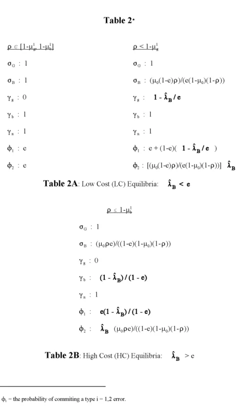
In this section we make some general observations about the equilibria we have identified, and discuss the implications of our results for designing administrative procedures. The reader may find it convenient to refer to the summary of equilibrium strategies listed in Table 2 in considering the following observations. Our first observation concerns the burden of proof borne by the respondent to have his request accepted by the commission. A comparison of the (LC) and (HC) equilibria characterized in Propositions 1 and 2 yields the following:
Observation 1: The burden of proof varies with the cost of the disclosure. In all cases the respondent must present evidence to avoid rejection. In addition, (i) if the cost of disclosure is high, the respondents request is accepted as long as he discloses with s = g. (ii) If the cost of disclosure is low, the burden of proof increases as the respondent may be rejected even if he discloses with s = g. The HC and LC equilibria are both supported by the belief that B types disclose with some strictly positive frequency in equilibrium. This means that the burden of proof for having an application accepted must be lower when disclosure costs are high in order to induce the B type respondent to disclose. When disclosure costs are low, the burden of proof can be increased without discouraging B type respondents from disclosing. Observation 1 is broadly consistent with a general principle of law which states that parties who have better and less costly access to information should bear a greater burden of proof and persuasion in deciding legal disputes. While this view24
is based on a normative argument, our observation is a prediction that parties with lower costs of presenting information will be expected to bear a greater burden of proof in equilibrium.
Our next observation evaluates the performance of the mandatory and voluntary presentation of evidence equilibria by comparing the expected cost of making type 1 and 2 errors in equilibrium. The total expected cost of type 1 and 2 errors, CE, is given by
CE = N E + N E1 1 2 2
where N is the probability of a type i=1,2 error in equilibrium.i 25
Recall that in the (HC) and (LC) voluntary disclosure equilibria, the respondent must disclose in order to have any chance of his application being approved. This does not imply that the voluntary and mandatory disclosure equilibria are equivalent however.
Observation 2: In equilibrium the expected cost of type 1 and 2 errors is less when disclosure is voluntary rather than mandatory.
One type of equilibrium is not uniformly better at minimizing both type 1 and 2 errors than another. However, direct calculations show that the expected cost, CE, of an incorrect decision is less under the (HC) and (LC) voluntary disclosure equilibria than under (M). Under (M) the respondent cannot signal his type by his decision to26
disclose as when disclosure is voluntary.27 This eliminates information that the commission may utilize to reach a more accurate decision.
In addition, since the respondent must disclose more often under (M), the total cost including the respondents cost of disclosure is higher. This point is best illustrated when e = 0 and evidence is perfectly informative. In this case, the argument for mandatory testing is perhaps most persuasive since type 1 and 2 errors are driven to zero. However, when disclosure is voluntary (as characterized in Proposition 2 for e = 0), B types never disclose, and respondents who fail to disclose are always rejected in equilibrium. Thus, the probability of type 1 and 2 errors are also driven to zero. However, with voluntary disclosure, B types incur no cost of testing in contrast to the M equilibria.
Safeguards in the Constitution and provisions in administrative law protect respondents from being compelled to present evidence in some instances. Aside28
from this protection of privacy, Observation 2 also implies that there are efficiency grounds for making the presentation of evidence voluntary. On the other hand, in some administrative settings where similar type cases occur frequently, it may be desirable to establish standard requirements for presenting evidence so that regulators may compare the merits of different cases more easily.29
Our next observation records the effect of a decrease in the cost of disclosing on equilibrium behavior. The cost of presenting evidence for a respondent depends on the commissions reporting requirements, what evidence is admissible, and the evidentiary standards for accuracy. The commissions generally seek to reduce the cost of manufacturing and presenting evidence to save resources, and to insure that the respondents right to due process is preserved. Aside from this, it seems that if respondents are more likely to present evidence if costs decrease, this should provide
the commissions with more information upon which to base its verdict. Surprisingly, this intuition is not borne out in the following:
Observation 3: Small reductions in the cost of disclosing only affect the accuracy of the verdicts in the semi-separating (LC) equilibria with D < (1-µ ) and in the (HC)1
g
equilibria. In these cases, a small reduction in costs C and CG B30
(i) increases the probability of type 1 errors and decreases the probability of type 2 errors in the (LC) and (HC) equilibria. As a result, the welfare of innocent respondents may be harmed as costs decline.
(ii) has no affect on CE for any equilibria.
To explain part (i) of Observation 3 note that the (LC) mixed strategy equilibria is supported by the belief that a certain fraction of B types disclose in equilibria. If the cost of disclosure decreases, B types are more likely to present evidence. This implies that the probability of acceptance must decrease if the expected equilibrium disclosure frequency for B types is to be maintained. A reduction in the probability of acceptance decreases type 2 errors (accepting an undesirable proposal) but it increases the probability of a type 1 error (rejecting a desirable proposal). This same type of intuition also explains the result for the case of (HC) equilibria.
Part (i) implies that under plausible conditions, good type respondents may be harmed by procedural or technological advances which reduce the cost of disclosing. This arises because the increase in a type 1 error resulting from the cost decrease may outweigh the reduction in disclosing costs. To see this, suppose that there is an equal reduction in disclosing costs for both type respondents so that -dCB
= -dC = -dC. The expected utility U to type G under the (LC) semi separatingG G
equilibrium for example is
where is the probability that the request is accepted when the respondent discloses with s=g. Differentiating U with respect to disclosing costs yieldsG
where the second line follows from substituting for and recognizing that e < ½.
There is a cruel irony with this result in that one might expect that a decrease in disclosing costs would help G type respondents who wish to demonstrate the
desirability of their requests. However, as disclosure costs decrease, the ability of31
G types to signal by disclosing more frequently than B types is diminished. The possibility that the G type respondent may suffer as disclosure costs decline is dramatically illustrated in the limiting case where disclosure costs tend to zero. In that case if the standard of proof for rejection is low with D < 1-µ , we find that in the (LC)1
g
equilibrium the respondent is always rejected even when he discloses with s = g. While this reduces type 2 errors to a minimum, the probability of a type 1 error is maximized. When testing costs converge to zero, the ability of G types to signal by testing more frequently than B types vanishes. Since the standard of proof for rejection is so low, both types are always rejected in equilibrium.32
Part ii of Observation 3 is best explained by considering one of the semi-separating equilibria such as (LC). In that case, the commission is indifferent to accepting and rejecting the request whenever disclosure reveals s = b. Consequently, CE is unaffected by the probability of acceptance. If the cost of disclosure decreases, it is necessary to decrease the probability of acceptance if type B is to disclose with the same frequency. But decreasing the probability of acceptance does not change CE and thus it is unaffected by changes in disclosure cost. This same argument applies to the other (HC) semi-separating equilibria as well.
The next observation characterizes how an increase in the accuracy of evidence affects the accuracy of the decisions reached through the administrative process.
Observation 4: An increase in the accuracy of evidence always reduces CE and it reduces the incidence of type 1 and 2 errors in most incidences.
As expected, increasing the accuracy of evidence results in more accurate decisions on average. However, in one instance, the (LC) equilibrium with D < 1-µ , the1
g
incidence of type two errors increases as the accuracy of the evidence increases. That equilibrium is sustained by the belief that the respondents request is accepted with a certain frequency whenever disclosure occurs with s = g. When disclosure accuracy increases, the commission becomes more likely to accept whenever s = g. On the other hand, when a greater percent of B types disclose, the commission becomes less likely to accept because the ability of G types to signal by the act of disclosure is diminished. Consequently, an increase in disclosure accuracy must be accompanied by an increase in the percent of B types who disclose in order for the commission to maintain its frequency of acceptance at the required equilibrium level. When more B types disclose, this has the effect of increasing the probability of type two errors, since they only arise when B types present evidence.33
While an increase in the accuracy of evidence may not always affect more accurate decisions, we find that decisions are unambiguously more accurate when the standard of proof for rejection declines. This is recorded in the following.
Observation 5: For the (LC) equilibria with D < 1-µ and the (HC) equilibria,1 i
decreases in the standard of proof, D, induce bad respondents to disclose less often, decrease the probability of type 2 errors, do not effect the probability of type 1 errors and decrease CE. Consequently, the expected costs of incorrect verdicts is reduced if the commission can commit itself to a less stringent standard of proof.34
The primary effect of a decrease in the standard of proof is to induce B type respondents to disclose less often. The intuition for this result is as follows. The (LC) mixing equilibrium is sustained by the belief that respondents who disclose with s = g have their requests approved with a certain frequency. The commission is more likely to reject a request when the standard of proof declines. On the other hand, the commission is more likely to approve a request if less B types disclose, since this allows G respondents to signal their type more effectively through the act of disclosure. Consequently, when the standard of proof declines, this must be accompanied by a decrease in the fraction of B types who disclose in order for the commission to willingly maintain the frequency of acceptance required for equilibrium. This same intuition applies for the other (HC) mixing equilibria.
It follows that as the frequency of B types disclosing is reduced, the incidence of type 2 errors declines, because such errors occur only when B types disclose. The incidence of type 1 errors is unchanged because the frequency of rejection is unaffected as the standard of proof declines. Consequently, the overall accuracy, as35
measured by -CE, increases as the standard of proof for rejection falls.
As we remarked earlier, evidentiary standards of proof for rejection are higher for those cases such as denaturalization and deportation proceedings, where type 1 errors are particularly costly. In such cases it is argued that type 1 errors may be avoided by raising the standard of proof, from a preponderance of evidence to the clear and convincing evidence standard for ruling against the respondent. Contrary to this view, Observation 5 implies that commissions may want, if possible, to resist the temptation of employing a higher standard of proof since this only serves to increase the incidence of type 2 errors while having no effect on the probability of type 1 errors. In addition, lowering the standard of proof might have beneficial deterrence36
effects of discouraging firms from violating regulations and policies in the first place.
V. Conclusion and Extensions
This paper analyzes how different procedures for presentation of evidence affect regulatory decisions and the welfare and efficiency properties these procedures exhibit. Modeling the administrative hearing as a game of imperfect information, we have examined the sequential equilibria of this game for its implications regarding (i) the advisability of making disclosure mandatory rather than voluntary, (ii) the burden
of proof borne by the respondent to prove his case, and (iii) the affect of increasing disclosure accuracy and decreasing disclosure costs on the outcome of the proceedings and the welfare of the respondents.
Our model of the administrative process is special and stylized, so that the policy conclusions which one draws from the model should be interpreted with care. For instance, several of our more interesting policy conclusions which appear in Observations 1-5 pertain to the mixed strategy equilibria characterized in Propositions 1 and 2. The interpretation of mixed strategies as representing the distribution of respondents who choose one pure strategy or another would be facilitated by assuming that respondents (of the same B or G type) also differ in their inherent cost of disclosing evidence. This would permit us to test the robustness of our results to alternative assumptions about factors affecting the costs of disclosure. Our model also abstracts from several factors which might be included in future work to enrich the analysis. For instance, we assume that commissioners are skilled in rationally updating and evaluating the evidence that is presented to them. It may be desirable to weaken this assumption if we wish to apply our analysis to trials in which jurists may consist of lay persons who are not necessarily adept at evaluating evidence. It is this concern about the ability of jurists to properly interpret some types of evidence which explains the more stringent standards for the permissibility of evidence in jury trials.37
Another important extension of our analysis would be to allow for the sequential presentation of evidence by the respondent. The respondent might also be allowed, at some cost, to control and to know the accuracy of the evidence before it is presented. In addition, it would be instructive to model the presentation of evidence by other parties besides the respondent who are interested in the outcome of administrative process.38
Finally, Owen and Braeutigan (1978), Noll (1989) and McCubbins et al. (1989) have argued informally that administrative procedures can be used to stack the deck in favor of special interest groups who have political clout. This is accomplished by making it easier for favored interests to intervene in the process and by placing the burden of proof on opposing interests. The model developed in this paper might provide a starting point for a formal analysis of how administrative procedures may be designed to affect certain regulatory outcomes.
1. It may be costly for the respondent to present evidence because of the difficulty of collecting data, the expense of hiring an expert witness, or the proprietary nature of the evidence to be disclosed.
2. The administrative law and procedures governing the behavior of Federal regulatory agencies is contained in the Administrative Procedures Act. An excellent account of the provisions of that act as well as general issues in administrative law is contained in Gellhorn and Boyer (1981).
3. See Yao and Dahdouh (1993, pg. 27) for a discussion of efficiency rationales for determining the burden of proof in regulatory proceedings.
4. Matthews and Postlewaite also allow for agents to acquire information, however unlike our analysis they assume that the agent is not initially privately informed about her type.
5. There are other no or partial disclosure results in the literature. For instance, Dye (1986) demonstrates that only favorable information is disclosed when disclosure is costly. Studies by Fishman and Hagerty (1990) and Dye (1985) analyze reporting procedures which allow for selective disclosure.
6. Our paper also follows recent papers exemplified by Bebchuk (1984), Grossman and Katz (1983), Nalebuf (1987), Png (1983, 1987), Reinganum (1988), Reinganum and Wilde (1986), Salant (1984), Sobel (1989) who employ game theory to study the resolution of legal disputes. However, unlike these papers which explain the incidence of pretrial negotiation and settlement, our paper focuses on the trial or hearing phase. Our work relates most closely to Rubinfeld and Sappington (1987) who examine how legal disputes are settled at trial by the relative effort allocated by both sides to persuade the jury.
7. Alternatively, the firm may be accused by the commission of violating a regulation or policy. During the hearing the firm is allowed to demonstrate that it is innocent of the violations that it is charged with. 8. Throughout we assume that the hearing is conducted in front of a regulatory commission although our analysis applies as well to trials that are tried in front of an administrative law judge.
9. For example the commission may use its prior knowledge of collusive behavior in the industry to form an initial opinion about whether a companys request to merge with one of its competitors is a good or bad request.
10. See Rubinfeld (1985) for an interesting discussion of the use of econometric tests in administrative proceedings.
11. Extending the model to permit sequential disclosure of several pieces of evidence is discussed in the concluding section.
12. We assume the commission may cross examine expert witnesses, or test the information presented for accuracy and authenticity.
13. The assumption that the evidence correctly signals g or b with equal probability is made only for simplicity. We ignore the possibility that the firm may know how the evidence will be interpreted and then disclose the evidence only if it signals that the request is good. In this case there would be no loss of generality in assuming that the evidence is always disclosed if it is public knowledge that the respondent knows the results of the disclosure. If the defendant were not to disclose the results, the commission would assume the evidence signaled b.
14. Our analysis is unchanged if we allow P to vary according to the type of respondent, provided ASSUMPTION 1 introduced below is satisfied.
15. We refer to a respondent who makes an desirable (undesirable) request as a good (G) (bad (B)) type respondent.
16. A similar assumption is employed in Rubinfeld and Sappington (1987) in their analysis of evidence in jury trials.
17. As explained in Gellhorn and Boyer (1981, Ch. 7), most routine regulatory decisions are made outside of formal hearings.
18. For instance most administrative hearings and civil proceedings require that a preponderance of evidence exist to rule against the respondent. In criminal trials and sensitive administrative hearing like deportation or denaturalization proceedings, the more stringent clear and convincing evidentiary standard is required to rule against the respondent. See pages 40-70 in Graham (1987).
19. This interpretation is consistent with Harsanyis (1973) purification approach to modeling mixed strategies. To interpret these strategies it is helpful to consider a slightly perturbed version of our model in which respondents of the same type have slightly different costs of presenting evidence. These differences may arise because respondents vary in their aversion to testifying, or to revealing personal or proprietary information. Similarly, we imagine that the commission may also differ slightly with respect to the standard of proof they require for any particular case. These differences may arise from disparities in how the commission interprets regulations or policies pertaining to each case.
Now consider the Bayesian equilibria for the following perturbed game in which respondents of a given type G or B, choose a pure strategy to present or not to present evidence based on their private cost of disclosure. The commission selects a pure strategy of whether or not to accept the respondents request based on his presentation of evidence and its standard of proof for rejection. Following Harsanyis purification approach one can show that the mixed equilibria we characterize in Propositions 1 and 2 may be interpreted as the limits of the pure strategies of the slightly perturbed game as the variation in costs and in the standard of proof goes to zero.
20. See Kreps and Wilson (1982) for a precise definition of sequential equilibrium.
21. Three signaling equilibria exist. When D > (1-µ ), there exists a pooling SE in which both types do0
not present evidence and the commission accepts the request. When D > (1-µ ) there exists a pooling SE1 b
in which both types present evidence, and the commission always accepts the request if the firm discloses, and rejects the request if there is no disclosure. Finally, if D > (1-µ ) there exists a semi-separating SE in0
which type G mixes between disclosing and not disclosing, and type B does not disclose. The commission mixes between acceptance and rejection if there is no disclosure, and accepts the request if the firm discloses. These equilibria are described further in Lewis and Poitevin (1993).
22. This is consistent with analyses of pretrial settlement which find that cases which are very likely to be settled in favor of the defendant are not brought to court.
23. Equilibria are unique, almost everywhere with the exception of the knife edge case of
where two equilibria exist. One equilibria is the limiting case of Proposition 1 and the other is the limiting case of Proposition 2 as e converges to .
24. See Yao and Dahdouh (1993) and the references cited therein for further elaboration on this view in the context of merger analysis.
25. One might add the defendants cost of testing to CE to derive a total cost measure by which to evaluate different testing procedures. However, scaling the costs of testing with the costs of type 1 and 2 errors to form a meaningful welfare measure seems problematic.
26. Recall that the (LC) equilibrium coincides with the (M) equilibria. For (1-µ ) # D # (1-µ ), while in1 1
g b
all other cases voluntary disclosure equilibria differ from the (M) equilibria.
27. Similar results are obtained in the analysis of disclosure by Dye (1985) and Fishman and Hagerty (1990) where information is revealed by the informed agents choice of how and what to disclose. 28. The Fourth Amendment to the Constitution bans unreasonable searches, and the Fifth Amendment prohibits compulsory self incrimination.
29. For instance, the Justice Department and the FTC routinely rely on sales and production data to construct indices of concentration which are used to determine whether proposed mergers between two or more firms are to be allowed.
30. In Observation 3, we assume the decrease in C (t=G,B) is sufficiently small so that the originalt
equilibrium still pertains as C changes. This comparative statics exercise is valid because there is a uniquet
equilibrium corresponding to a given set of parameters except when .
31. Observation 3 applies only to small decreases in disclosing costs. Large decreases in disclosing costs may cause a discrete shift in equilibria, and the effects on disclosing frequency, on the probability of type 1 and 2 errors and on CE appear to be ambiguous.
32. When the standard of proof for rejection is higher with D 0 [1-µ , 1-µ ] then the respondent is rejected1 1 g b
only when disclosure signals s = b, independent of the cost of disclosure.
33. The probability that a B type who discloses will be rejected remains the same as the accuracy of disclosure increases. Thus, as more B types disclose the probability of type 2 errors increases, since respondents are always rejected when they dont disclose.
34. Changes in D have no effect on the (LC) equilibrium when D 0 [1-µ ,1-µ ].1 1 g b
35. Notice from Propositions 1 and 2 that the probability of rejection is locally independent of D in all equilibria.
36. We are grateful to David Sappington for suggesting this to us.
37. Milgrom and Roberts (1986) analyze situations in which jurists are not able to evaluate information in a perfectly rational (Bayesian) fashion. See the discussion in Gellhorn and Boyer (1981, pp. 202-207) on how the admissibility of evidence varies between jury trials and administrative proceedings. 38. For models of this kind see the interesting analyses by Milgrom and Roberts (1986) and by Lippman and Seppi (1993) on the disclosure of information by interested parties.
N= the probability of commiting a type i = 1,2 error. % 1
Table 2
%% D0[1-µ , 1-µ ]1 1 D< 1-µ1 g b g FG : 1 FG : 1 FB : 1 FB : (µ (1-e)D)/(e(1-µ )(1-D))0 0 (g : 0 (g : (b : 1 (b : 1 (n : 1 (n : 1 N1 : e N1 : e + (1-e)( ) N2 : e N2: [(µ (1-e)D)/(e(1-µ )(1-D))]0 0Table 2A
: Low Cost (LC) Equilibria: D#1-µ1 b FG : 1 FB : (µ De)/((1-e)(1-µ )(1-D))0 0 (g : 0 (b : (n : 1 N1 : N2 : (µ De)/((1-e)(1-µ )(1-D))0 01
− µ
01
− µ
1 bFigure 1: M Equilibria
*s = g
s = b
ρ
0
1
{
1
− µ
1{
{
g1
1− µ
b1
− µ
0γ
g= =
γ
b1
γ
g= =
γ
b0
γ
g=
0
,
γ
b=
1
Figure 2: LC Equilibria:
s = g
s = b
ρ
0
1
− µ
1g1
γ
g=
0
[
]
ρ∈ −1 µ1 1−µ1 g, bγ
b=
1
ρ
γ
g=01
− µ
1 g1
− µ
01
1− µ
bFigure 3: LC Equilibria:
s = g
s = b
ρ
0
1
Figure 4: HC Equilibria:
ρ≤ −1 µ1 b ρ≤ −1 µ1 gρ
γ
b=
1
( )
γ
g∈
01
,
1
− µ
1 g1
− µ
01
1− µ
bs = g
s = b
ρ
0
1
( )
γ
b∈
01
,
ρ
Bibliography
Banks, J.S. and Sobel, J. Equilibrium Selection in Signaling Games. Econometrica, Vol. 55 (1987), pp. 647-662.
Bebchuk, L.A. Litigation and Settlement under Imperfect Information. RAND Journal of Economics, Vol. 15 (1984), pp. 404-415.
Cho, I.K. and Kreps, D.M. Signaling Games and Stable Equilibria. Quarterly Journal of Economics, Vol. 102 (1987), pp. 179-221.
Cooter, R.D. and Rubinfeld, D.L. Economic Analysis of Legal Disputes and Their Resolution. Journal of Economic Literature, Vol. 27 (1989), pp. 1067-1097.
Dye, R.A. Strategic Accounting Choice and the Effects of Alternative Financial Reporting Requirements. Journal of Accounting Research, Vol. 23 (1985), pp. 544-574.
Dye, R.A. Proprietary and Nonproprietary Disclosures. Journal of Business, Vol. 59 (1986), pp. 331-366.
Farrell, J. Voluntary Disclosure: Robustness of the Unraveling Result, and Comments on Its Importance. In Antitrust and Regulation, R. Grieson, ed. (Lexington: Lexington Books, 1986).
Fishman, M.J. and Hagerty, K.M. The Optimal Amount of Discretion to Allow in Disclosure. Quarterly Journal of Economics, (1990), pp. 427-444. Gellhorn, E. and Boyer, B. Administrative Law and Process, 2nd Ed, (St. Paul, MN:
West Publishing Co., 1981).
Graham, M.H. Federal Rules of Evidence in a Nutshell, 2nd Ed. (St. Paul, MN: West Publishing Co., 1987).
Grossman, S.J. The Informational Role of Warranties and Private Disclosure about Product Quality. Journal of Law and Economics, Vol. 24 (1981), pp. 461-483.
Grossman, S.J. and Hart, O.D. Disclosure Laws and Takeover Bids. Journal of Finance, Vol. 35 (1980), pp. 323-334.
Grossman, G.M. and Katz, M.L. Plea Bargaining and Social Welfare. American Economic Review, Vol. 7(4) (1983), pp. 749-757.
Harsanyi, J. Games with Randomly Distributed Payoffs: A New Rationale for Mixed-Strategy Equilibrium Points. International Journal of Games Theory, Vol. 2 (1973), pp. 1-23.
Klevorick, A. and Rothschild, M. A Model of the Jury Decision Process. Journal of Legal Studies, Vol. 8 (1979), pp. 141-164.
Kreps, D.M. and Wilson, R. Reputation and Imperfection Information. Journal of Economic Theory, Vol. 27(2) (1982), pp. 253-284.
Lewis, T.R. and Poitevin, M. The Disclosure of Evidence in Trial Proceedings. Working Paper, University of Florida, 1993.
Lippman, B. and Seppi, D. Robust Inferences in Communication Games with Partial Provability. Working Paper, 1993.
Matthews, S. and Postlewaite, A. Quality Testing and Disclosure. RANDJournal of Economics, Vol. 16 (1985), pp. 328-340.
Milgrom, P.R. Good News and Bad News: Representation Theorems and Applications. Bell Journal of Economics, Vol. 12 (1981), pp. 380-391. Milgrom, P.R. and Roberts, J. Relying on the Information of Interested Parties.
RANDJournal of Economics, Vol. 17 (1986), pp. 18-32.
Nalebuff, B. Credible Pretrial Negotiation. Rand Journal of Economics, Vol. 18(2) (1987), pp. 198-210.
Owen, B. and Braeutigam, The Regulation Game, Ballinger (1978).
Png, I.P.L. Strategic Behavior in Suit, Settlement, and Trial. Bell Journal of Economics, Vol. 14(2) (1983), pp. 539-550.
Png, I.P.L. Litigation, Liability, and Incentives for Care. Journal of Public Economics, Vol. 34(1) (1987), pp. 61-86.
Priest, G. and Klein (1984), The Selection of Disputes for Litigation Journal of Legal Studies, Vol. 13 (1984).
Reinganum, J.F. Plea Bargaining and Prosecutorial Discretion. American Economic Review, Vol. 78(4) (1988), pp. 713-728.
Reinganum, J.F. and Wilde, L. Settlement, Litigation and the Allocation of Litigation Costs. RANDJournal of Economics, Vol. 17 (1986), pp. 557-566. Rubinfeld, D.L. Econometrics in the Courtroom. Columbia Law Review, Vol. 85(5)
(1985), pp. 1048-1097.
Rubinfeld, D.L. and Sappington, D. Efficient Awards and Standards of Proof in Judicial Proceedings. RAND Journal of Economics, Vol. 18 (1987), pp. 308-315.
Salant, S.W. Litigation of Settlement Demands Questioned by Bayesian Defendants. Social Science Working Paper No. 516, California Institute of Technology, March 1984.
Schrag, J. and Scotchmer, S. Character Evidence in Hierarchical Justice. Working Paper No. 187, Graduate School of Public Policy, University of California, Berkeley, 1991.
Sobel, J. An Analysis of Discovery Rules. Law and Contemporary Problems, Vol. 52(1) (1989).
Yao, D. and Dahdouh, T. Information Problems in Merger Decision Making and Their Impact on Development of an Efficiencies Defense. Antitrust Law Journal, Summer (1993), pp. 23-45.
Appendix
In the proofs to follow, we denote the expected equilibrium payoff to the respondent as
a function of the commission's equilbrium strategy by for t = B,G. We define
as the commission's expected payoff along the equilibrium path if the outcome of the
disclosure decision is s' 0 {n,b,g}.
Proof of Lemma 1: The proof goes by contradiction.
Suppose there exists a SE with equilibrium strategies
There are two possibilities,
and .
(1) Suppose . Since only type B tests, we must have that
The payoffs to the bad type respondent from disclosing and not disclosing
are
Since we must have which is impossible given that C > 0B
by ASSUMPTION 1.
(2) Suppose now that . We must first show that .
µ > µ where µ is the revised probability that the respondent has good type conditioned on theg b s'
disclosure outcome s'. We have that , ,
, and . Now consider two possibilities.
i) If we have that which implies that
This implies that and hence -µ E > -(1-µ )E . Thusb 1 b 2
. Under our initial supposition that , we must have that .
But , is impossible by an argument similar to that made in case (1). Consequently,
if , it must be the case that , contradicting our initial supposition that
(ii) If , then and thus
Furthermore, since we have Since
we have that This implies that .
Hence and the commission's payoff must therefore satisfy
which implies We then have We know
that It is easy to show that, if µ >n
µ . But this contradicts the inequalities above, and hence implies b
Now we show that is impossible. Since , we
Since , we have that which implies that
ASSUMPTION 1 then implies that
This requires that thus contradicting the condition
Hence,
Q.E.D.
Proof of Lemma 2: Suppose there exists a pure strategy separating SE. The full separation of
types implies that, in equilibrium, the type G is accepted and the type B is rejected with probability
one. This implies that type B does not disclose in equilibrium and therefore that type G does
disclose with probability one. But since P-C > 0, type B always has the incentive to mimic typeB
G, thus destroying the separating equilibrium.
Q.E.D.
Proof of Lemma 3: Consider a candidate SE in which This implies
for t 0 {B,G} which requires
This implies that and
ASSUMPTION 1 then implies that
Since we have that which implies that
Therefore, and then . But this is inconsistent with
Hence, there can be no equilibrium in which the two types mix between disclosing and not
disclosing with positive probability smaller than one.
Q.E.D.
Proof of Proposition 1: Consider the following strategies.
(i) (1-µ ) 1 #D# (1-µ )1
g b
The respondent, regardless of type, plays Ft = 1, t = B,G. The commission plays (n = (b = 1 and (g = 0. We now show that these strategies can form part of a SE.
Given the commission's equilibrium strategy, the respondent of type G is strictly better
off disclosing, since < when which
is implied by The respondent of type B is strictly better off
disclosing since < when Each
respondent type's equilibrium strategy is therefore a best reply to the commission's equilibrium
strategy.
Given the respondent's equilibrium strategy, the commission believes that the
respondent has type G with probability µ if the test result is s 1 0 {b,g}. Since 1-µ 1#D# 1-µ , the1
s g b
respondent is rejected if and only if the disclosure outcome is g. Off the equilibrium path, the
commission believes with probability that the respondent has type B if he does not
disclose, and therefore, it rejects the request. The commission's equilibrium strategy is therefore
a best reply to its own beliefs and the respondent's equilibrium strategy. Furthermore, the
commission updates its priors according to Bayes rule on the equilibrium path. The outcome
described in the proposition can then be supported as a SE.
(ii) D# (1-µ )1 g
The respondent of type G plays FG = 1. The respondent of type B plays FB = < 1 under the assumption in the proposition. The commission plays (n = (b
= 1 and (g = 1- . We now show that these strategies can form part of a SE.
Given the commission's equilibrium strategy, the respondent of type G is strictly better
off disclosing, since < The respondent of
type G is indifferent between disclosing and not disclosing, since =
The respondent's equilibrium strategy is therefore a best reply
to the commission's equilibrium strategy.
Given the respondent's equilibrium strategy, the commission believes that the
respondent is good with probability µ = 0 if he does not disclose. Therefore, the commissionn
optimally rejects the respondent if he does not disclose. The commission believes with probability
µ = g = 1-D that the respondent is good if he discloses good
evidence. The commission is therefore indifferent between accepting and rejecting, and its
strategy is therefore optimal. The commission believes with probability µ =b
= < 1-D that the
respondent is good if he discloses bad evidence. The commission then optimally rejects the
beliefs and the respondent's strategy. Furthermore, the commission updates its priors according
to Bayes rule on the equilibrium path. The outcome described in the proposition can then be
supported as a SE.
Q.E.D.
Proof of Proposition 2: Consider the following strategies.
The respondent of type G plays FG = 1. The respondent of type B plays FB = < 1 under the assumption of the proposition. The commission plays (n
= 1, (g = 0, and (b = when . We now show that these strategies can form part of a SE.
Given the commission's equilibrium strategy, the type G respondent is strictly better off
disclosing than not disclosing since <
The respondent of type B is indifferent between
disclosing and not disclosing, since =
The respondent's equilibrium strategy is therefore
a best reply to the commission's equilibrium strategy.
Given the respondent's equilibrium strategy, the commission believes with probability
optimally rejects the respondent if he does not disclose. The commission believes with probability
µ = g = > 1-D that the
respondent has good type if he discloses a good outcome. In that case, the commission optimally
accepts the respondent. The commission believes with probability µ =b
= 1-D that the respondent has good type if he discloses a bad
outcome. The commission is therefore indifferent between acceptance and rejection, and its
strategy is therefore optimal. The commission's equilibrium strategy is therefore a best reply to
its own beliefs and the respondent's strategy. Furthermore, the commission updates its priors
according to Bayes rule on the equilibrium path. The outcome described in the proposition can
then be supported as a SE.