Modelling and Simulation of a Two wheeled vehicle with suspensions by using Robotic Formalism

HAL Id: hal-00583154

https://hal.archives-ouvertes.fr/hal-00583154

Submitted on 5 Apr 2011

HAL is a multi-disciplinary open access archive for the deposit and dissemination of sci-entific research documents, whether they are pub-lished or not. The documents may come from teaching and research institutions in France or abroad, or from public or private research centers.

L’archive ouverte pluridisciplinaire HAL, est destinée au dépôt et à la diffusion de documents scientifiques de niveau recherche, publiés ou non, émanant des établissements d’enseignement et de recherche français ou étrangers, des laboratoires publics ou privés.

Modelling and Simulation of a Two wheeled vehicle with

suspensions by using Robotic Formalism

Salim Maakaroun, Philippe Chevrel, Maxime Gautier, Wisama Khalil

To cite this version:

Salim Maakaroun, Philippe Chevrel, Maxime Gautier, Wisama Khalil. Modelling and Simulation of a Two wheeled vehicle with suspensions by using Robotic Formalism. IFAC World Congress, Aug 2011, Milano, Italy. �hal-00583154�

Modeling and Simulation of a Two wheeled vehicle with suspensions by using

Robotic Formalism

Salim Maakaroun*+, Philippe Chevrel*+

Maxime Gautier*, Wisama Khalil*

*Institut de Recherche en Communications et Cybernétiques de Nantes (IRCCyN) 1,Rue de la Noë, B.P. 92101, 44321 Nantes Cedex 3, France

(Salim.Maakaroun@irccyn.ec-nantes.fr Wisama.khalil@irccyn.ec-nantes.fr Maxime.gautier@irccyn.ec-nantes.fr) +Ecole des Mines de Nantes, Département d'Automatique-Productique

4 rue Alfred Kastler - La Chantrerie, B.P. 20722, 44307 Nantes cedex 3, France (Philippe.chevrel@emn.fr)

Abstract: Models, simulators and control strategies are required tools for the conception of secure and

comfortable vehicles. The aim of this paper is to present a systematic approach to develop models for dynamic vehicle, focusing on a two wheeled vehicles whose body involves six degrees of freedom. The resulting model is sufficiently generic to perform simulation of realistic cornering and accelerating behaviour in various situations. It may be used in the context of motorcycle modeling, but also in various situations (e.g. for control application) as simplified model for 3 or 4 wheeled (tilting) cars. The approach is based on considering the vehicle as a multi-body poly-articulated system and the modeling is carried out using the robotics formalism based on the modified Denavit-Hartenberg geometric description. In that way, the dynamic model is easy to implement and the system can be used for control applications.

Keywords: Modeling, Simulation, Automotive, Robotics, Simulators, Dynamics, Vehicle

1. INTRODUCTION

Modeling and simulating vehicle dynamics are fundamental tools for vehicles research and development. They allow understanding the dynamics of vehicles and improving the design in order to ensure the major challenge of having safe, comfortable and economic vehicles. Hence, the goal is to build a mathematical model that illustrates significant aspects of the physical dynamics and then facilitate performance analysis and assess design tradeoffs.

In the literature, most of the models proposed are developed for control applications (Sharp, 1971). They are centred on motorcycle behaviours, and neglect some essential aspects such as gyroscopic effect on the steering handle bar or pitch motion due to the suspension system (Weir 1978), (Katayama et al, 1985).

Lately, some advanced models have been developed using multi body systems. R.S Sharp provided his model by using Autosim software with a description lack on the applied method (Sharp et al, 2001). Later, Cossalter et al developed a model based on Lagrange Formalism that consist on interconnected rigid bodies together with suspensions and other flexible components, supplemented by sophisticated tire and engine models (Cossalter et al, 2002). This formulation uses absolute coordinates that do not depend on the topological structure of the system. However, this technique leads to a complicated model, hard to implement and requires complex numerical algorithm to solve the DAE’s (Shabana, 1994).

Therefore to model a complex system (Rajamani, 2006), (Kiencke et al, 2000) in 3D motion, we claim that it is preferable to proceed in a systematic geometrical description,

based on the modified Denavit Hartenberg parameterization (Khalil et al 1986). This description allows to automatically calculate the symbolic expression of the geometric, kinematic and dynamic models by using a symbolic software package as SYMORO+ (Symbolic Modeling of Robots) (Khalil et al, 1997). This formulation leads to a minimum set of differential equations from where the constraint equations for the mechanical system are automatically eliminated.

This paper concentrates on developing a dynamical model for a two wheeled vehicle (called bicycle) by applying recursive methods used in robotics. The approach elaborates systematically the symbolic equations of motion and makes the implementation of the dynamic model easier.

This work can be extended for various complex vehicles, such as narrow electric tilting car, specifically Smera Car from Lumeneo (Lumeneo) and (Maakaroun, 2010a, b). The paper is organized as follows: the global method is described in section 2.1 and applied to the bicycle system in section 2.2. A dynamic model is then elaborated using a recursive Newton-Euler based Algorithm (Khalil et al, 1987) in section 3. Finally, Simulations results are illustrated and commented and conclusions are done. The paper ends with a summarize conclusion.

2. GEOMETRICAL DESCRIPTION OF THE CAR

2.1 Robotic representation of a multi body system

The bicycle is considered as a mobile robot which is a tree-structured multi body system composed of n bodies (links) where the chassis is the mobile base and the wheels are the

terminal links. The links are numbered consecutively from

the base to the terminal links. Each body Cj is connected to

its antecedent Ci (i=a(j)) with a joint that represents a

translational or rotational degree of freedom and can be elastic or rigid. a(j) denotes the link antecedent to link j, and consequently a(j) < j .A body can be virtual or real; the virtual bodies are introduced to describe joints with multiple degrees of freedom like ball joint or intermediate fixed frames.

The frame Ri (Oi, xi, yi, zi) which is attached to the body Ci is

defined as following:

The zi axis is along the axis of joint i, the uj axis is defined as

the common normal between zi and zj. The xi axis is along the

common normal between zi and one of the succeeding z axis,

where link i is the antecedent of link j and the origin Oi is the

intersection of zi and xi.

The homogeneous transformation matrix i_T

j between two

consecutive frames Ri and Rj is expressed as a function of the

following six parameters (Fig. 1):

• γj: angle between xi and uj about zi

• bj: distance between xi and uj along zi

• αj: angle between zi and zj about uj

• dj: distance between zi and zj along uj

• θj: angle between uj and xj about zj

• rj: distance between uj and xj along zj

Fig. 1. Geometric parameters

The generalized coordinate of joint j is denoted by qj, it is

equal to rj if j is translational and θj if j is rotational. In

(Fig.1), since xi is taken along uk, the parameters γk and bk are

equal to zero. We define the parameter σj = 1 if joint j is

translational and σj = 0 if joint j is rotational. If there is no

degree of freedom between two frames that are fixed with

respect to each other, we take σj =2. In this case, the time

derivative of qj is zero.

2.2 Application for the model

Our model is composed of 12 bodies (Fig.2 & Fig.3) connected by 11 joints:

- C1 is the chassis

- C3 and C9 are the front and rear suspensions. Their

movement is represented by prismatic flexible joints.

- C6 is the rear driving wheel and C11 is the front steering

wheel.

- C4 is the steering column

- C2, C5, C7, C8, C10, C12 are virtual bodies fixed to other links

by blocked joints.

Fig. 2. Multi body description of the bicycle

Fig. 3. Shape of the bicycle

The description of the bicycle considered as a multi body poly articulated system uses the Denavit and Hartenberg (MDH) notations that are commonly used in robotics (Fig.4). The chassis motion is described with Euler coordinates while all the other links are described with the generalized Lagrangien coordinates.

According to MDH description and SYMORO+, C0 is the

base attached to the ground. The structure is defined as a

robot with a mobile base by considering C1 attached to C0 via

a blocked joint.The inertial parameters of this base are those

of C1 and the speed and the acceleration are then the ones of

the chassis described in his own frame.

Let Rf be a fixed reference frame attached to the ground. The

body C1 with a location ζ (i.e. position & orientation) gives

the system posture in the frame Rf.

The movement of the chassis in this mixed Euler-Lagrangien model is given by:

⎥ ⎥ ⎥ ⎦ ⎤ ⎢ ⎢ ⎢ ⎣ ⎡ = ⎥ ⎥ ⎥ ⎦ ⎤ ⎢ ⎢ ⎢ ⎣ ⎡ = ⎥ ⎥ ⎥ ⎦ ⎤ ⎢ ⎢ ⎢ ⎣ ⎡ = 1 1 1 1 1 1 1 1 1 1 1 1 1 1 1 1 1 1 1 1 1 1 1 1 _{, ,} z y x z y x z y x V V V V ω ω ω ω ω ω ω ω & & & & & & & &

Where Vx1, Vy1 and Vz1 are respectively the longitudinal,

lateral and vertical translational speed of the chassis.

Where

ω

₁and

ω

&₁are the angular velocity and accelerations of

the chassis.

According to this description, the geometric parameters of the tree structure are shown in table 1 and the bicycle motion is completely described by the vector q of the 11 generalized coordinates:

[

]

T

q

=

ξ

ξ

₁ ;

ξ

₁

=

[

r

₃

r

₉

q

₆

q

₁₁

q

₄

]

- ξ [1x6] is the posture of the chassis (position & orientation)

- r3 and r9 are the length of the suspensions,

- q6 and q11 are the angular positions of the two wheels with

respect to their revolute axis,

- q4 is the steering angle.

Table 1. Geometric Parameters of the modal

3. DYNAMIC MODEL

3.1 Dynamic parameters

For each link there are 14 standard dynamic parameters (Gautier et al, 1990) composed of 10 standard inertial parameters (Table 2):

- Jj = [XXj XYj XZj YYj YZj ZZj ]: the six coefficients of the

inertia matrix of link j given in the frame Rj ,

- MSj = [MXj MYj MZj]: the three components of first moment

of link j around the origin of the frame j,

- Mj: the mass of link j

Table 2. Dynamic parameters of the modal

For each actuated joint j, we introduce:

- Iaj as the total inertia of the rotor of motor and the drive

transmission.

- Fvj, Fsj as the viscous and coulomb friction parameters.

For a flexible joint, we define:

- Kj as the stiffness of the joint j

For joint 3 and 9 we add K3, K9, Fv3 and Fv9 to the parameters

listed in Table 2. These parameters represent respectively the stiffness of the springs and the dampers of the suspensions.

3.2 External Forces

The external forces applied to the bicycle, which have the most significant impact on vehicle dynamics, are the contact forces between the ground and the tires. These external forces can be modeled (Pacejka, 2002), estimated (Canudas, 2003) or measured at the center of the wheels by using dynamometric wheels.

Aerodynamic forces also have an effect on the vehicle behavior, particularly at high speed (> 90 Km/h).

3.3 Euler-Lagrange Dynamic model

The mixed Euler-Lagrange model is obtained from two recurrences of the algorithm of Newton-Euler in the following way (Khalil, 2002):

The forward recursive equations can be summarized as follows: for j= 1 to n, we calculate the total forces and moments on each link

] [ j j j j i j j j j i i i j i j j j j j i j j j i i i j i j a q a q A a q A & && & & & × + + = + = = ω σ ω ω σ ω ω ω ω (1) j j j j j j j j j j j j j j j j j j j j j j j j j j j j i j j j j j j i i i i j i j j j V MS J J M MS V M F a q a q P V A V & & & & && & & × + × + = Υ + = × + + Υ + = ) ( ) 2 ( ) ( ω ω ω ω σ (2)

The backward recursive equations can be summarized as follows: for j= n to 1, we calculate the forces and moments

exerted on body Bj by its antecedent Bi .

) ˆ ( ( ) ( ) ( ) ( ) ( ) ( ) ( ) ( j s j j s j j s j s j s j s i ej j j j j j j j j i j i j s j s j ej j j j j j f P m A m M m f A f f f F f + + + = = + + =

∑

∑

(3) Where:

- ω and _j ω& are respectively the angular velocity and j

the angular acceleration of body j.

- Fj and Mj are respectively the total forces and moments

applied on the body j with respect to Oj.

- j

Y

_j

_{= &}

j

ω

ˆ +

_j j

ω

ˆ

_j j

ω

ˆ

_j (4)

- j_Aiand

i

j_{P are respectively the orientation 3x3 matrix}

and the position vector of the origin Oi of frame Ri in

j a(j) σj γj bj αj dj θj rj 1 0 2 0 0 0 0 0 0 2 1 2 0 0 0 Lf 0 0 3 2 1 0 0 π 0 π r3 4 3 0 0 0 0 0 q4 0 5 4 2 0 0 π/2 0 0 0 6 5 0 0 0 0 0 q 6 π 0 7 5 2 0 0 π/2 0 -Ra 8 1 2 0 0 0 -Lr 0 0 9 8 1 0 0 π 0 π R9 10 9 2 0 0 π/2 0 0 0 11 10 0 0 0 0 0 q11 π 0 12 10 2 0 0 π/2 0 -Ra j XX XY XZ YY YZ ZZ MX MY MZ M 1 XX1 XY1 XZ1 YY1 YZ1 ZZ1 MX1 MY1 MZ1 M1 2 0 0 0 0 0 0 0 0 0 0 3 0 0 0 0 0 0 0 0 0 M3 4 0 0 0 0 0 0 0 0 0 0 5 0 0 0 0 0 0 0 0 0 0 6 XX6 0 0 YY6 0 ZZ6 0 0 0 M6 7 0 0 0 0 0 0 0 0 0 0 8 0 0 0 0 0 0 0 0 0 0 9 0 0 0 0 0 0 0 0 0 M9 10 0 0 0 0 0 0 0 0 0 0 11 XX11 0 0 YY11 0 ZZ11 0 0 0 M11 12 0 0 0 0 0 0 0 0 0 0 Rj.

- (5)

- Jj , MSj and Mj are described in section 3.A

Rj

ied by ked joint), all terms multiplied

[

]

⎥ ⎥ ⎥ ⎦ ⎤ ⎢ ⎢ ⎢ ⎣ ⎡ − − − = = 0 0 0 ˆ ; 1 0 0 x y x z y z T j j_a ω ω ω ω ω ω ω

- s(j) indicates the bodies whose antecedent is body

- fej and mej are the external forces and moments appl

body Cj on the environment.

When σj is equal to 2 (a bloc

by σj or σ are eliminated. _j

The inverse dynamic model gives the joint torques as a function of the joint coordinates, speeds and accelerations.

The joint forces or torques are obtained by projecting fj or mj

on the joint axis zj and by taking into account the effects of

friction and elasticity as follows:

j j j j e j vj j sj f j e j f j j j T j j_{f + m a} = Γj (

σ

j j

σ

j j) off q K q F q sign F + = Γ + = Γ Γ + Γ + & & ) ( (6)

For the body C1 there is no projection on the joint axis, so the

equations of the chassis will be represented by the total forces

f1 and moments m1 exerted by link 0 on link 1. Thus the NE

equations of the chassis are expressed in terms of Euler

variables

[

1 ₁

]

1 1 1 1 _,ω,ω & & V

.

(7)

f1 and m1 are equal to zero because there is no body

el (IDM) of a tree structure with a

(8)

- A(11x11) is the inertial matrix of the system

olis and gravity

is the Jacobian matrix and Jfe is the vector of

locity and accelerations all the

4. SIMULATOR

To predict the behavi we made a simulator

[ ]

⎥ ⎦ ⎤ ⎢ ⎣ ⎡ = × 1 1 1 1 1 6 0 m f

antecedent to the chassis. The inverse Dynamic mod mobile base can be written as:

(

)

(

q

q

H

q

A

&& +

=

Γ

)

,

,

,

,

,

,

,

(

)

(

)

,

K

F

F

g

f

q

q

q

f

f

q

J

q

v s e t t t e t T t t t t

&&

&

&

=

+

- H(11x1) is the vector of centrifugal, Cori

terms.

- J(11xp)

generalized efforts representing the projection of the external forces and torques on the joint axes.

- p: number of the components of fe

- q_t,q& ,_t q&&_t are the angular position, ve

of joints including the variables of the chassis such as:

[

]

T t x y z r r q q q q = θ ϕ ψ _{3 9 6 11 4}

[

]

T z y x z y x t V V V w w w r r q q q q 1 _{1 3 9 6 11 4} 1 1 1 1 1 1 1 1 1 1 & & & & & & =

[

]

T z y x z y x t V V V w w w r r q q q

q&& = 1&1 1&1 1&1 1& 1 1& 1 1&1 &&3 &&9 &&6 &&11 &&4

our of the bicycle,

by using the dynamic model obtained from the equation of

Newton-Euler. The simulator architecture is described in figure 5:

Fig. 5. Simulator architecture

4.1 Direct Dynamical model

The direct dynamical model, used in the simulation, gives the joint accelerations as a function of joint positions, velocities torques, and external wrenches. It is represented by the following relation:

]

)

(

)

,

(

[

)]

(

[

)

,

,

,

,

,

,

,

(

1 e t T t t t v s e t t t

f

q

J

q

q

H

q

A

K

F

F

g

f

q

q

g

q

−

−

Γ

=

Γ

=

−

&

&

&&

(9) As we said in Section 3.3, the torques related to the variables of the chassis are zero and the torques of passive joints are zero, we can conclude:

) 1 6 (

0

)

6

:

1

(

=

_x

Γ

and Γ(11)=0

Moreover, by adding the stiffness and the friction coefficient to the suspensions joint as in section 3.1, the torque of joint 3 and 9 will be equal also to zero.

Hence the global vector of torques will be written as follows:

[

]

T 4 11 0 0 0 0 0 0 0 0 0 Γ Γ = Γ

The matrix A can be calculated by the algorithm of Newton-Euler, by noting from the relation (8) that the ith column is equal to Γ: ) 0 , 0 , 0 , 0 , 0 , , 0 , ( ) (:,i f qt ui A = ( ui is t 10) he unit (11 x 1) vector, whose elements are zero except an be obtained with the the ith element which is equal to 1.

The calculation of the vector H c

Newton-Euler method, by noting that H = Γ if: ) , , , , 0 , 0 , , (q q g F F K f H = t &t s v (11)

The Matrix J can be calculated

(12)

e is the unit (p x 1) vector, wh

5. SIMULATION

In mean to show t e bicycle in three

ted. nds significantly T _{as follows:} ) 0 , 0 , 0 , 0 , , 0 , 0 , ( ) (:, _{t i} T _{i f q e} J = i

the ith element which is equal to 1. ose elements are zero except

he behaviour of th dimensions, two test scenarios are considered. The following assumptions are used:

- The aero dynamical forces are neglec -The behaviour of the ground vehicles depe

on the nature of the interaction between the tire and the road. As said in section 3.2, this interaction has been modeled and

Trajectory Direct Dynamical Model t

q

t

q&

Integrators + Transformation matrix External Wrenches Scenario t

q&

&

Visualization Desired Torques

the well known and widely used one is Pacejka Magic formula. This model captures in steady-state motion, the tire/road forces and moments, in algebraic equations form with respect to load, longitudinal slip and lateral slip. Among a six components of the tire/road contact wrench, we have considered the principal ones: longitudinal and lateral forces. -To keep the tires in contact with the ground, we must add two constraints to the dynamical model. Therefore, the vertical velocity and acceleration of the contact tire/road with respect to the reference frame must be equal to zero.

⎤

⎡

f

_V

(13)

0

) 3 ( 12 ) 3 ( 7

₌

_Φ

₌

⎥

⎥

⎦

⎢

⎢

⎣

f

V

q

&

t t t t f f q dt d q q dt d V V dt d & && &) ( ) ( ) 3 ( 12 ) 3 ( 7 _{= Φ =Φ + Φ} ⎥ ⎥ ⎦ ⎤ ⎢ ⎢ ⎣ ⎡

₍₁₄₎ quation (8) becomes: Where: x

resents the vector of the efforts transmitted by And the direct dynamical model for simulation will be:

(15)

5.1 First Scenario: longitudinal behaviour

In this scenario, the bicycle is subject to traction torque E

λ

T e t T t t t t

q

H

q

q

J

q

f

q

A

+

+

+

Φ

=

Γ

(

)

&&

(

,

&

)

(

)

- Φ(2 11) - λ(2x1) rep

joints to respect the constraints.

] ) ( ) , ( [ 0 ) ( ) 2 2 ( e t T t t x t t Aq _{H q q J q f} q − − Γ ⎥ ⎥ ⎦ ⎢ ⎢ ⎣ Φ Φ = ⎥ ⎦ ⎤ ⎢ ⎣ ⎡ & &&

λ

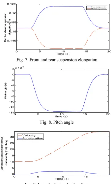
1 T _⎤ ⎡ −

applied at the rear wheel. The shape of this torque stimulates an accelerated phase then a decelerated one as shown in Fig 6. The trajectory is a straight line with an initial velocity equal to 10 m/s. When the bicycle accelerates, a transfer load will occur from the front to the rear part of the vehicle. Consequently, the length of the front suspension will increase, and the one of the rear suspension will decrease (Fig 7.). Hence, a negative pitch angle will appear with respect to its revolute axis which is taken to the left as in Fig 8. The velocity and the acceleration of the center of gravity with respect to the reference frame are shown in Fig.9.

0 5 10 15 20 -700 -600 -500 -400 -300 -200 -100 0 100 0 5 10 15 20 0.145 0.15 0.155 0.16 0.165 Time (s) F ront an d r ear s us pens ion el on ga tio n ( m ) front suspension Rear suspension

Fig. 7. Front and rear suspension elongation

0 5 10 15 20 -14 -12 -10 -8 -6 -4 -2 0 2 x 10-3 time (s) P itc h angl e ( rd)

Fig. 8. Pitch angle

0 5 10 15 0 5 10 15 20 25 30 Time (s) Longi tudi nal ac ce le ra tion ( m /s 2) and v el oc ity ( m /s ) o f c .g Velocity Acceleration

Fig. 9. Longitudinal velocity of c.g

5.2 Second Scenario: lateral behaviour

In this scenario, the system is subject to a desired steering torque applied on the steering column to follow the trajectory imposed by a steering desired angle (Fig 10). We consider in this case that the longitudinal velocity is constant and equals to 3 m/s. However, to maintain the stability, the bicycle must tilt into the corner such that the resultant force of the lateral acceleration and the weight of the vehicle is along the vertical axe of the vehicle. The desired tilt angle will be the roll of the bicycle and it will be equal to:

Time (s) R ear T or que (N )

Fig. 6. Rear Torque

θ

=

a

tan(

f

V

_x1

ψ

&

/

g

)

(16)

In order to get that, a simple PD controller is used to stabilize the roll dynamics to any desired tilt angle. The controller’s output represents the required tilting torque to stabilize the bicycle and it will be applied to the dynamical model by

putting it equal to Γ5 .

Fig 10 and Fig 11 illustrate the steering desired angle and the trajectory while the last have the shape of double bend. The roll, yaw and desired tilt angle are shown in Fig. 12

Motorcycle Riders,” Vehicle System Dynamics: Intern- 0 5 10 15 20 25 30 -0.4 -0.3 -0.2 -0.1 0 0.1 0.2 0.3 Time (s) D esi re d S te eri ng a ng le (r

d) ational Journal of Vehicle Mechanics and Mobility,

17(4), 211-229.

Khalil, W., Kleinfinger, J. (1986). "A new geometric notation for open and closed-loop robots," Robotics and Auto-

mation. Proceedings. 1986 IEEE International Confe re- nce on , vol.3, no., pp. 1174- 1179.

Khalil, W. and Kleinfinger, J.(1987) “Minimum operations and minimum parameters of the dynamic model of tree Fig. 10. Desired steering angle

structure robots,”IEEE J. Robot.Autom., vol. RA-3, no. 6, pp. 517–526. 0 10 20 30 40 50 0 5 10 15 20 25 30 35 40 X Longitudinal distance of c.g (m) Y L ate ra l d is ta nce o f c .g (m

) Khalil, W. and Creusot, D. (1997). “Symoro+: A system for

the symbolic modeling of robots,” Robotica, vol. 15, no. 2, pp. 153–161.

Khalil, W. and Dombre, E. Modeling, Identification and

Control of Robots. London : Hermès Penton, 2002.

Kiencke, U. and Nielsen, L. (2000). Automative Control

Systems for Engine, Driveline and Vehicle. New York:

Springer-Verlag. Fig. 11. Trajectory of c.g in the horizontal plan

Lumeneo, www.lumeneo.fr.

Maakaroun, S, Khalil, W. and al. (2010a). “Geometrical

0 5 10 15 20 25 30 -0.5 0 0.5 1 1.5 2 2.5 Time (s) R ol l, Y aw a nd D es ire d T ilt an gl e ( rd ) Roll angle Yaw Angle

Desired tilt angle Model of a New Narrow Tilting Car”, in Proc. 15th Int

Conf. on Methods and Models in Automation and Robotics. Poland

Maakaroun, S, Khalil, W. and al. (2010b). “Dynamic Model of a New Narrow Tilting Car”, submitted to. IEEE int

Conf. on Robotics and automation, Shanghai

Pacejka. H.B,(2002). Tyre and Vehicle Dynamics. Oxford, U.K.: Butterworth-Heinemann.

Fig. 12. Roll, Yaw and Desired tilt angle _{Shabana, A. A. (1994). Computational Dynamics. Johan}

Wiley and Sons.

Sharp, R. S. (1971). “The stability and control of motor- 6. CONCLUSIONS

cycles,” Journal Mechanical Engineering Science, Based on a mixed Euler-Lagrange formulation, a two

wheeled vehicle dynamic model was developed for simulation’s purpose and some dimensioning and control applications. Future works will consist on applying this technique on more complex and sophisticated vehicles as narrow tilting cars such as the Smera from our collaborator Lumeneo. Two approaches will be compared : i) a bottom up one consisting to analyze the ability of the simplified model proposed in the present paper to give realistic results with ad hoc parameters using identification from experimental data, ii) a top down one, showing how to simplify the complete model for control purpose..

vol. 13, no. 5, pp. 316 – 326.

Sharp, R. S., (2001). “Stability, control and steering responses of motorcycles,” Vehicle System Dynamics, vol. 35(4-5), pp. 291–318.

Weir, D.H. and Zellner, J. W., (1978) “Lateral directional Motorcycle Dynamics and rider control,” SAE paper No.780304

Appendix A. SYTEM VARIABLES AND PARAMETERS x, y, z: longitudinal, lateral and vertical distance of the centre of gravity with respect to the reference frame.

θ, φ, ψ: roll, pitch and yaw of the bicycle Ra: Radius of the wheels: 0.275 m

REFERENCES h: 0.625 m :height of c.g of bicycle from ground

Lf = Lr = 0.85 m: longitudinal distance from c.g to front and

rear wheels; g = 9.81 m/s2 _{: gravitational constant}

Canudas deWit, C., Tsiotras, P. and al, (2003).“Dynamic

friction models for road/tire longitudinal interaction,” _M

1= 1000 Kg: mass of the chassis

Veh.Syst. Dyn., vol. 39, no. 3, pp. 189–226. _M

3 = M9 = 1.32 Kg: mass of a suspension

Cossalter, V., Lot, R. (2002). “A motorcycle multi-body _M

6 = M11 = 10 Kg: mass of a wheel

model for real time simulations based on the natural _XX

1=43.3 Kg m2 : roll moment of inertia of bicycle

coordinates approach,” Vehicle System Dynamics, vol. _YY

1=254 Kg m2 : pitch moment of inertia of bicycle

37, no. 6, pp. 423–447. _ZZ

1=270 Kg m2 : yaw moment of inertia of bicycle

Gautier, M. and Khalil, W. (1990), “direct calculations of _XY

1= XZ1= YZ1= MX1= MY1= MZ1=0

minimum set of inertial parameters of serial robots,” _XX

6 = YY6 = XX11 = YY11 = 0.207 Kg m2

IEEE Trans. On Robotics and Automation, Vol. RA- _ZZ

6 = ZZ11 = 0.378 Kg m2

6(3), p. 368-373. _K

3 = K9 =50000 N/m: stiffness of a suspension

Rajamani R. (2006). vehicle dynamics and control, Springer. _F

v3 = Kv9 =5200 Ns/m: damping coefficient of a suspension