Motion detection: Fast and robust algorithms for embedded systems

(1)

HAL Id: hal-01130889

https://hal.archives-ouvertes.fr/hal-01130889

Submitted on 12 Mar 2015

HAL is a multi-disciplinary open access

archive for the deposit and dissemination of

sci-entific research documents, whether they are

pub-lished or not. The documents may come from

teaching and research institutions in France or

abroad, or from public or private research centers.

L’archive ouverte pluridisciplinaire HAL, est

destinée au dépôt et à la diffusion de documents

scientifiques de niveau recherche, publiés ou non,

émanant des établissements d’enseignement et de

recherche français ou étrangers, des laboratoires

publics ou privés.

Motion detection: Fast and robust algorithms for

embedded systems

Lionel Lacassagne, Antoine Manzanera, Antoine Dupret

To cite this version:

Lionel Lacassagne, Antoine Manzanera, Antoine Dupret. Motion detection: Fast and robust

algo-rithms for embedded systems. International Conference on Image Processing (ICIP), Nov 2009, Le

Caire, Egypt. �10.1109/ICIP.2009.5413946�. �hal-01130889�

(2)

MOTION DETECTION: FAST AND ROBUST ALGORITHMS FOR EMBEDDED SYSTEMS

L. Lacassagne

IEF/AXIS – Digiteo Labs – Universit´e Paris Sud

A. Manzanera

UEI – ENSTA – Paris Tech

ABSTRACT

This article introduces a new hierarchical version of a set of motion detection algorithms called Σ∆. These new algo-rithms are designed to preserve as much as possible the com-putational efficiency of the basical Σ∆ estimation, in order to target real-time implementation for low power consumption processors and embedded systems.

Index Terms— Motion detection, Sigma-Delta filtering, Embedded systems, Real-Time implementation.

1. INTRODUCTION

The growing interest for developing fully automatic video surveillance systems has recently renewed the interest for fast and reliable motion detection algorithms. Such algorithms must partition the pixels of every frame of the image sequence into two classes: the background, corresponding to pixels be-longing to the static scene (label: 0), and the foreground, cor-responding to pixels belonging to a moving object (label: 1).

A motion detection algorithm must discriminate the mov-ing objects from the background as accurately as possible, without being too sensitive to the sizes and velocities of the objects, or to the changing conditions of the static scene. For long autonomy and discretion purposes, the system must not consume too much computational resources (energy and circuit area) [1]. As it involves a great amount of data -like any image processing module - the motion detection is certainly the most computationally demanding function of a video surveillance system.

Background subtraction techniques have been the object of much attention for years [2]. Recently, we have proposed a new type of methods based on Σ∆ estimation [3]. These methods are very attractive from a computational point of view since they work on any size fixed-point arithmetic using only comparison, increment and absolute difference, while being as robust as other mono-modal statistical estimation methods (e.g. Gaussian estimation), whose computation is much more costly.

Different modified versions of the basical Σ∆ algorithm have been proposed since then. The purpose of this paper is to review and compare them and also to introduce a new hierarchical version.

2. Σ∆ BACKGROUND SUBTRACTION The basic principle of the Σ∆ algorithm is to estimate param-eters of the background using Σ∆ modulation, which is a very common tool in analog-to-digital conversion: Considering a time-varying signal ft(continuous or discrete), we estimate a

discrete signal dtby quantizing the time indexes {ti}i∈N, and

then performing at every time index i the following update formulas:

If dti−1 < ftithen dti = dti−1− ε else dti= dti−1+ ε

where ε is the discretization step (least significant bit) of dt.

In Σ∆ background subtraction, the input signal is the value of every pixel over time It, from which we compute

the first Σ∆ background estimator Mt. Then the values of

the absolute differences |It− Mt| are used to compute the

second Σ∆ background estimator Vt, which is a parameter of

dispersion.

2.1. Basical Σ∆ algorithm

Algorithm 1: Basical Σ∆

foreach pixel x do [step #1: Mtestimation]

1 if Mt−1(x) < It(x) then Mt(x) ← Mt−1(x) + 1 2 if Mt−1(x) > It(x) then Mt(x) ← Mt−1(x) − 1 3 otherwise Mt(x) ← Mt−1(x) 4

foreach pixel x do [step #2: Otcomputation]

5

Ot(x) = |Mt(x) − It(x)|

6

foreach pixel x do [step #3: Vtupdate]

7 if Vt−1(x) < N × Ot(x) then Vt(x) ← Vt−1(x) + 1 8 if Vt−1(x) > N × Ot(x) then Vt(x) ← Vt−1(x) − 1 9 otherwise Vt(x) ← Vt−1(x) 10

Vt(x) ← max(min(Vt(x), Vmax), Vmin)

foreach pixel x do [step #4: ˆEtestimation]

11

if Ot(x) < Vt(x) then ˆEt(x) ← 0 else ˆEt(x) ← 1

12

In the basical version (Alg. 1), the Σ∆ background Mt

and Σ∆ variance Vt are updated every frame, according to

the comparison with the current image Itand current absolute

difference Otrespectively. N is an amplification factor for

Vt, allowing then to compute the motion label ˆEtby simply

comparing Otand Vt(typical values of N are between 1 and

(3)

overflow of Vtthat could happens if some pixels are saturated

(due to sensor over-exposition). Their typical values are 2 and 2m− 1 respectively (where m is the number of bits of the representation). Note that this clipping is a modification not present in the original version [3].

2.2. Improved algorithm: conditional Σ∆

Algorithm 2: Conditional Σ∆

foreach pixel x with do [step #1’:conditional Mtupdate]

1 if ˆEt−1(x) = 0 then 2 if Mt−1(x) < It(x) then Mt(x) ← Mt−1(x) + 1 3 if Mt−1(x) > It(x) then Mt(x) ← Mt−1(x) − 1 4 otherwise Mt(x) ← Mt−1(x) 5 else 6 Mt(x) ← Mt−1(x) 7

foreach pixel x do [step #2: Otcomputation]

8

Ot(x) = |Mt(x) − It(x)|

9

foreach pixel x do [step #3: Vtupdate]

10 if Vt−1(x) < N × Ot(x) then Vt(x) ← Vt−1(x) + 1 11 if Vt−1(x) > N × Ot(x) then Vt(x) ← Vt−1(x) − 1 12 otherwise Vt(x) ← Vt−1(x) 13

14

15

16

The conditional version (Alg. 2 and Fig. 1) uses relevance feedback from the estimated position of the moving objects at the previous frame, given by ˆEt−1. It consists in updating the

Σ∆ background Mtand/or the variance Vtonly for the pixels

x considered background (i.e. where ˆEt−1(x) = 0). It

pre-vents moving object from integrating the background and/or modifying the noise variance [4].

Σ∆

_Eˆ_t ˆ Et−1 It Mt Vt−1 Mt−1 Vt Fig. 1. conditional Σ∆ 2.3. Zipfian estimation

The Zipfian version (Alg. 3) [5] is based on the relation be-tween the Σ∆ estimation and the statistical estimation, using

a Zipf-Mandelbrot distribution, which implies that the updat-ing frequency of the background should be proportional to the dispersion of the distribution (variance). In that version, we first compute a threshold which varies according to the frame index t: ρ is the value of the index modulo 2m (m is the number of bits of the representation). π is the value of the greatest power of 2 which divides ρ. Finally the thresh-old σ is equal to 2m_{divided by π. The result is that pixels x}

such that Vt(x) > 2m−k will be updated every 2k−1frames,

for k ∈ {1, m}. To avoid auto-reference, the variance Vt

is updated using a constant period TV (usually a power of 2

between 1 and 64). TV, like the amplification parameter N ,

can be automatically adjusted using a simple noise estimation method, which consists in counting the number of isolated pixels in the estimated labels ˆEt.

Algorithm 3: Zipfian estimation [step #0: variance threshold computation]

1

find the greatest 2p

that divides (t mod 2m) 2

set σ = 2m/2p 3

foreach pixel x do [step #1”:conditional Mtestimation]

4 if Vt−1(x) > σ then 5 if Mt−1(x) < It(x) then Mt(x) ← Mt−1(x) + 1 6 if Mt−1(x) > It(x) then Mt(x) ← Mt−1(x) − 1 7 otherwise Mt(x) ← Mt−1(x) 8 else 9 Mt(x) ← Mt−1(x) 10

[ foreach pixel x do [step #2: Otcomputation]

11

Ot(x) = |Mt(x) − It(x)|

12

foreach pixel x do [step #3”: update Vtevery TV frames]

13 if t mod TV = 0 then 14 if Vt−1(x) < N × Ot(x) then 15 Vt(x) ← Vt−1(x) + 1 if Vt−1(x) > N × Ot(x) then 16 Vt(x) ← Vt−1(x) − 1 otherwise Vt(x) ← Vt−1(x) 17

18

19

20

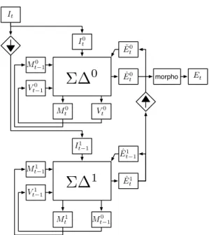
2.4. New hierarchical algorithm

The hierarchical algorithm (Fig. 2) is a bi-level version of Σ∆ filtering. Each Σ∆ block implements the basic algorithm #1 of the algorithm #3. Both blocks are using conditional up-date. At the low level it is a conditional temporal update: M_t1 and Vt1are updated depending on ˆE1t−1. At the high level, it

is a conditional spatial update: Mt0 and Vt0are updated

de-pending on ˜Et0, the oversampling binary mask of ˆEt1. The

subsampling factor is in the range [2, 10] and is set accord-ingly to the “size” of the clutter noise. Finally, a morpho-logical post-processing is applied in two steps. The first one

(4)

It M0 t−1 V1 t−1 ˆ E1 t−1 ˆ E1 t

Σ∆

1

M1 t M1 t−1 I1 t−1 morpho Mt0−1 Vt0−1 M0 t Vt0 I0 t ˆ E0 t Et ˜ E0 t

Σ∆

0

Fig. 2. hierarchic Σ∆

removes stand-alone pixels that are considered as noise, the second one is a 3 × 3 morphological closing.

3. BENCHMARK

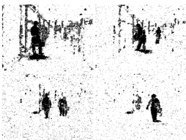
Fig. 3. Hall sequence, images 38, 91, 170, 251

In order to evaluate the impact of the modifications on the performance of these algorithms, a RoC analysis has been done with the Hall sequence (Fig. 3) than can be considered as a difficult sequence because of the radial movement of non-rigid objects (people). The Ground Truth has been drawn for 4 images of that sequence. Given T P the True Positive, T N the True Negative, F P the False Positive and F N the False Negative, we compute the Matthews Correlation Coefficient

(Eq. 1) instead of accuracy or product of T P ratio by T N ratio because the two classes (motion and background) are of very different size. It returns a value between −1 (perfect inverse segmentation) and +1 (perfect segmentation) while 0 signifies a wrong segmentation.

M CC = T P × T N − F P × F N

p(T P + F P )(T P + F N)(T N + F P )(T N + F N) (1) A set of 32 algorithms (combinations of parameters) has been evaluated. Figures (Tab. 1) are provided for only four of them: Σ∆ is the basic algorithm (Fig. 4), Σ∆+Zipf (Fig. 5) is the basic algorithm with Zipfian estimation, Conditional Σ∆ (Fig. 6) is the best mono-level algorithm with conditional update (with or without Zipfian estimation) and Hierarchical Σ∆ (Fig. 7)is the best two-level algorithm with conditional update. For this benchmark, the decimation factor for sub-sampling and oversub-sampling was set to 8 and the Zipfian Vt

update period TV was set to 4.

algorithm 38 91 170 251 average

M CC without morphological post processing

Σ∆ 0.495 0.347 0.169 0.282 0.323

Σ∆+Zipf 0.676 0.600 0.366 0.308 0.487

ConditionalΣ∆ 0.424 0.533 0.555 0.590 0.526 HierarchicalΣ∆ 0.644 0.663 0.468 0.415 0.548

M CC with morphological post processing

Σ∆ 0.811 0.657 0.372 0.596 0.609

Σ∆+Zipf 0.830 0.728 0.547 0.449 0.639

ConditionalΣ∆ 0.754 0.764 0.530 0.385 0.608 HierarchicalΣ∆ 0.816 0.827 0.686 0.582 0.728 Table 1. Results: M CC scores for 4 Σ∆ algorithms with/without morphological post processing

Considering first, the results without post morphological processing, each evolution has better results than the previous one. The best conditional version is obtained with Zipfian es-timation combined with the conditional update of Mtand Vt.

The best hierarchical version is obtained with the best con-ditionalversion combined with a conditional update of Mt1

at low level. Considering then the results with morphologi-cal post processing, all results are in progression except for image # 170 that corresponds to radial movement of the first person. Both visual and numerical results enforce the use of morphological post-processing (Fig. 8) to remove remaining noise. Another benchmark, not presented here, has been done on a sequence with cars. The results were better but harder to differentiate, as such a kind of sequence is easier to segment.

4. CONCLUSION

We have presented a new hierarchical and conditional mo-tion detecmo-tion algorithm based on an evolumo-tion of previous Σ∆ algorithms. Preliminary results show better (visual and

(5)

Fig. 4. basic Σ∆

Fig. 5. Σ∆ + Zipf

quantitative) performances for difficult sequences with radial movement and non-rigid object. As its complexity remains low this algorithm is well suited for very light embedded sys-tems. Future work will consider other difficult sequences with the presence of clutter like snow, rain or moving trees.

5. REFERENCES

[1] L. Lacassagne; A. Manzanera; J. Denoulet; A. M´erigot, “High perfor-mance motion detection: Some trends toward new embedded architec-tures for vision systems,” JRTIP, october 2008.

[2] M. Piccardi, “Background subtraction techniques: a review,” in Confer-ence on Systems, Man and Cybernetics. IEEE, 2004, vol. 4, pp. 3099– 3104.

[3] J. Richefeu A. Manzanera, “robust and computationally efficient motion detection algorithm based on sigma-delta background estimation,” in ICVGIP. IEEE, 2004.

[4] L. Lacassagne J. Denoulet, G. Mostafaoui and A. M´erigot, “Implement-ing motion markov detection on general purpose processor and associa-tive mesh,” in CAMP. IEEE, 2005.

[5] A. Manzanera, “Sigma-delta background subtraction and the zipf law,” in CIARP. LNCS, 2007, vol. 28-2, pp. 42–51.

Fig. 6. conditional Σ∆

Fig. 7. Hierarchical Σ∆