Development of a robust microfluidic electrochimical cell for biofilm study in controlled hydrodynamic conditions

Development of a Robust Microfluidic

Electroch

emical Cell for Biofilm Study in Controlled

Hydrodynamic Conditions

Thèse

Mirpouyan Zarabadi

Doctorat en chimie

Philosophiæ doctor (Ph. D.)

Québec, Canada

Development of a Robust Microfluidic

Electrochemical Cell for Biofilm Study in

Controlled Hydrodynamic Conditions

Thèse

Mirpouyan Zarabadi

Sous la direction de :

Jesse Greener, directeur de recherche

Steve Charette, codirecteur de recherche

Résumé

Le domaine de la bioélectrochimie a actuellement un grand impact sur les nouvelles biotechnologies, notamment les dispositifs médicaux aux points de service et la détection bioélectrochimique. D'autre part, les systèmes émergents de bioénergie offrent de nouvelles opportunités pour se passer des produits pétroliers classiques grâce à des approches alternatives plus durables sur le plan environnemental. En tant que telle, la branche de la bioélectrochimie traitant des systèmes énergétiques est sur le point d’avoir un impact incontestable sur les concepts d’énergie verte et de bioénergie. Pour faciliter ces études et d'autres, les systèmes bioélectrochimiques (BES), qui utilisent des composants biologiques tels que des bactéries (souvent appelées biocatalyseurs), sont de plus en plus développés et miniaturisés pour une nouvelle série de biotechnologies.

Cette thèse porte sur la fabrication et la fonctionnalité d’un « système

microfluidique électrochimique à trois électrodes » pour l’étude de biofilms de

différentes bactéries (électroactives et non-électroactives) à l’aide de différentes techniques électrochimiques. Ces biofilms ont été largement étudiés par des techniques électrochimiques et d’imagerie microscopique (microscopie optique et électronique). Cette thèse pourra potentiellement ouvrir la voie à une nouvelle vague de développements de biocapteurs électrochimiques, tout en offrant des avancées scientifiques spécifiques dans les études de biocapacité de biofilm, de biorésistance, de pH du biofilm, de dépendance nutritionnelle de l'activité du biofilm et de la cinétique de respiration bactérienne.

Abstract

The area of bioelectrochemistry is currently making the greatest impact in new biotechnology, including point of care medical devices and bioelectrochemical sensing. On the other hand, emerging bioenergy systems offer new opportunities to move away from conventional petroleum products toward more environmentally sustainable alternative approaches. As such, the branch of bioelectrochemistry dealing with energy systems is poised to have an undoubtable impact on green-energy and biogreen-energy concepts. To facilitate these and other areas of study, bioelectrochemical systems (BESs), which use biological components such as bacteria (often referred to as biocatalysts) are increasingly being developed and miniaturized for a new round of biotechnology.

This PhD thesis focuses on fabrication and functionality of a “three-electrode

electrochemical microfluidic system” for biofilm studies of different bacteria (electroactive and non-electroactive) using different electrochemical techniques. They were broadly studied by electrochemical and microscopic imaging (optical and electron microscopy) techniques. This thesis can potentially open the way for a new wave of electrochemical biosensor development, while offering specific scientific advances in studies of biofilm biocapacitance, bioresistance, biofilm pH, nutrient dependency of biofilm activity and bacterial respiration kinetics.

Table of contents

Résumé ... ii

Abstract ... iii

Table of contents ... iv

List of Figures ... ix

List of tables ... xxiii

List of abbreviations ... xxiv

Acknowledgment ... xxvi

Foreword ... xxvii

Introduction ... 1

Chapter 1. Background ... 2

1.1 Electrochemical cell ... 2

1.1.1 Electrochemical cell configuration ... 2

1.1.2 Electrochemical techniques ... 3

1.1.2.1 Cyclic voltammetry (CV) ... 3

1.1.2.2 Chronoamperometery (CA) ... 5

1.1.2.3 Electrochemical impedance spectroscopy (EIS) ... 6

1.2 Bioelectrochemistry ... 8

1.2.1 Bioelectrochemical sensing ... 9

1.2.1.1 Biomolecule sensing with CV and EIS ... 10

1.2.1.2 Electrochemical sensing of planktonic and sessile bacteria ... 12

1.2.2 Bioelectrochemical systems (BES) ... 14

1.2.2.1 Electroactive bacteria ... 15

1.2.2.2 Microbial fuel cells (MFCs) ... 17

1.2.2.3 Microbial 3-electrode cells (M3Cs) ... 20

1.2.2.4 Kinetic and environmental effects on EAB electrode respiration ... 21

1.2.2.5 Biocatalytic kinetic measurements in flow ... 24

1.3 Microfluidics ... 25

1.3.1 Principles, characteristics and benefits of microfluidics ... 26

1.3.2 Microfluidic fabrication and methods ... 29

1.3.2.2 Casting and bonding ... 32

1.3.3 Bacteria and their biofilms studied with microfluidics ... 33

1.3.4 Biofilms in microfluidic electrochemical cells ... 34

1.4 Scope of thesis ... 35

Chapter 2. Hydrodynamic effects on biofilms at the biointerface using a microfluidic electrochemical cell: case study of Pseudomonas sp. ... 38

2.1 Résumé ... 39

2.2 Abstract ... 40

2.3 Introduction ... 41

2.4 Experimental section ... 42

2.4.1 Fabrication of a microfluidic flow cell ... 42

2.4.2 Bacteria and solution preparation ... 45

2.4.3 Channel inoculation by laminar flow-templating ... 45

2.4.4 Optical microscopy ... 46

2.4.5 Electrochemical impedance spectroscopy (EIS) ... 46

2.4.6 Attenuated total reflection infrared spectroscopy (ATR-IR) ... 47

2.5 Results and discussion... 48

2.5.1 Flow templated biofilm growth ... 48

2.5.2 Electrochemical impedance spectroscopy on templated biofilms and verification ... 50

2.5.3 Biofilm resistance and capacitance under changing flow conditions ... 54

2.6 Conclusion ... 59

2.7 Acknowledgments ... 60

2.8 Supporting information ... 60

2.8.1 Calibration of the Au pseudo-reference electrode ... 60

2.8.2 Elements to the equivalent electrical circuits for biofilms on electrode surfaces ... 62

2.8.3 A modified electrical equivalence circuit for biofilms consisting of separated colonies ... 63

2.8.4 Expansion of templated growth region in time ... 64

2.8.6 Quantifying the restructuring process at the attachment surface by CLSM

measurements ... 67

2.8.7 Measurement of shifting biofilm at the attachment surface using CLSM .. 69

Chapter 3. Flow-based deacidification of Geobacter sulfurreducens biofilms depends on nutrient conditions: A microfluidic bioelectrochemical study ... 70

3.1 Résumé ... 71

3.2 Abstract ... 72

3.3 Introduction ... 73

3.4 Experimental section ... 76

3.4.1 Bacterial preparation ... 76

3.4.2 Device fabrication and anaerobic environment ... 76

3.4.3 Electrochemical measurements ... 78

3.4.4 Samples preparation for SEM imaging ... 78

3.5 Results and discussion... 78

3.6 Conclusion ... 89

3.7 Acknowledgments ... 90

3.8 Supporting Information ... 90

3.8.1 Bulk electrochemical set-up ... 90

3.8.2 Hydrodynamic calculations ... 91

3.8.3 Reference electrode calibration ... 92

3.8.4 Stability of formal potential under long durations and different flow rates 93 3.8.5 Set up of electrochemical microfluidic device and anaerobic container ... 95

3.8.6 Effect of starvation and nutrient-limited conditions ... 95

3.8.7 Biofilm activity and electric current for different [Ac] and Q ... 97

3.8.8 SEM Imaging ... 98

Chapter 4. Toggling Geobacter sulfurreducens metabolic state reveals hidden behaviour and expanded applicability to sustainable energy applications ... 99

4.1 Résumé ... 100

4.2 Abstract ... 101

4.4 Results and discussion... 104

4.5 Conclusion ... 114

4.6 Supporting information ... 115

4.6.1 Device fabrication and experiment methodology ... 115

4.6.2 Hydrodynamic considerations at and away from the working electrode . 117 4.6.3 Bacterial preparation ... 119

4.6.4 Reference electrode calibration and stability ... 120

4.6.5 Device inoculation and growth ... 120

4.6.6 Identification of cytochrome c formal potential by CV ... 122

4.6.7 Fluctuations in electrical current for different metabolic activity regimes 122 4.6.8 Efficiency of acetate digestion ... 124

Chapter 5. A Generalized Kinetic Framework Applied to Whole‐Cell Bioelectrocatalysis in Bioflow Reactors Clarifies Performance Enhancements for Geobacter Sulfurreducens Biofilms... 126

5.1 Résumé ... 127

5.2 Abstract ... 127

5.3 Introduction ... 128

5.4 Results and discussion... 131

5.5 Conclusion ... 136

5.6 Supporting information ... 137

5.6.1 Bacterial preparation ... 137

5.6.2 Microfluidic device fabrication, anaerobic environment and inoculation . 137 5.6.3 Flow rate vs. time ... 141

5.6.4 SEM sample preparation ... 141

5.6.5 The Michaelis-Menten and Lilly-Hornby kinetics ... 142

5.6.6 Verification of efficient electron transfer kinetics ... 143

5.6.7 Initial biofilm growth in microfluidic electrochemical cell ... 146

5.6.8 Bulk set-up for bacterial growth and measurements of KM ... 146

5.6.9 Influence of flow on reactor parameters ... 147

5.6.10 Trends in the device reaction capacity ... 148

Chapter 6. Perspectives and future works ... 151

6.1 Master curve of {flow rate – nutrient concentration – bacterial activity} in G. sulfurreducens biofilm ... 151

6.2 Spectroelectrochemistry for electroactive bacteria studies... 153

6.3 Direct interspecies electron transfer (DIET) ... 154

Conclusion ... 158

List of Figures

Figure 1.1 (a) One cycle of potential scanning showing the initial potential (more positive potential) to the switching potential (more negative potential) and then, coming back to initial potential value. (b) The resulting cyclic voltammogram showing the measurement of the peak currents and peak potentials... 5 Figure 1.2 (a) potential of the electrode versus time. At t = 0, a constant

potential, V(app), is applied on the electrode and it is maintained constant during

measurement. (b) Curve of chronoamperometery, which shows changes of current versus time. ... 6 Figure 1.3 (a) Typical Nyquist plot based on Randles circuit model. (b) Typical Bode plot based on Randles circuit model. ... 7 Figure 1.4 (a) Randles equivalent circuit (b) Nyquist curve of Randles circuit ... 8 Figure 1.5 Scheme of an electrochemical biosensor. Biological sensing elements are coupled to working electrode. These traduce the signal to deliver a readable output. ... 9 Figure 1.6 A schematic of a generic biofilm and composition of the EPS. ... 13 Figure 1.7 The simplified mechanism for acetate metabolism in G. sulfurreducens bacteria with Fe (III) serving as the electron acceptor. C-cyt and OmcB are c-type cytochrome and outer membrane c-type cytochrome, respectively. Higher electrochemical redox potentials toward outer membrane c-type cytochrome allow the electrons to pass through the membranes. ... 16 Figure 1.8 A conventional microbial fuel cell consisting of an anaerobic chamber (anode, left) and aerobic chamber (cathode, right), connected by proton exchange membrane (green dash line). The electrons passed through the external circuit reaching the cathode to form water. EABs are accumulated on the surface of anode electrode.. ... 18

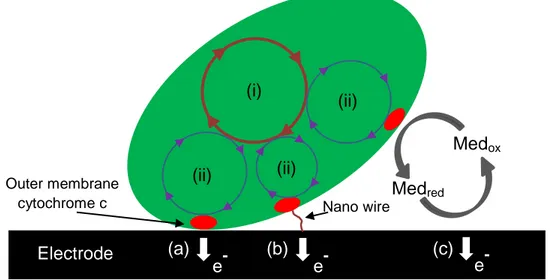
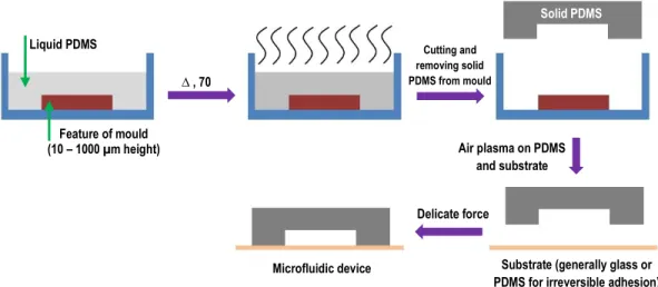
Figure 1.9 Shows direct electron transfer mechanism between electroactive bacteria and anode electrode surface by (a) outer membrane bound cytochromes and (b) electronically conducting nanowires (c) Shows MET mechanism with two proposed procedures: shuttling via outer membrane cytochromes and via periplasmic redox couples. (i) represents TCA cycle for bacteria and (ii) is internal electron transfer from TCA cycle to outer membrane cytochromes c. ... 19 Figure 1.10 A microbial 3-electrode device connected to a potentiostat featuring an electroactive biofilm (brown ovals on the surface of working electrode) that is set up in a single-chamber electrochemical cell. Counter electrode supports a hydrogen evolution reaction. ... 21 Figure 1.11 (a) A typical Michaelis–Menten curve based on current output of BES in function of nutrient concentration for electroactive bacteria, assuming non-limiting electron transport. (b) The Nernst–Michaelis–Menten curve for electroactive bacteria in high nutrient concentration (non-limiting nutrients).. ... 22 Figure 1.12 A representation of laminar flow with separate flow layers (left) and a turbulent flow with crossed-mixed flow layers (right). ... 26 Figure 1.13 (a) Side view of velocity profile and (b) shear rate distribution in a simple geometry with laminar flow. ... 28 Figure 1.14 A schematic of positive and negative photoresist patterning. Based on which photochemical reactions occur during light exposure time, positive or negative features can be made on the substrate. Final mould will be ready after washing with the developer solution and cleaning removable portions.. ... 31 Figure 1.15 A schematic of PDMS baking and casting for microfluidic device fabrication... 32 Figure 2.1 Device fabrication. (a) Cross-section view of the mold (diagonal cross-hatch) with a raised feature that defines the microchannel, which is fixed to the bottom of a container (dashed). (b) Two 3 mm wide graphite electrodes

(black) and a 5 mm wide gold electrode (green) were placed on top of the mold channel feature. (c) PDMS (grey) with cross-linker were poured over the mold/electrode assembly. (d) Zoomed cross-section view from the marked region in (c) of the microfluidic device after removal from the mold with embedded electrodes and sealing to a glass microscope slide (blue). Device includes inlets (I1, I2), and outlet (O). Cleaning process described in text not shown. (e) Bird’s eye view of the microfluidic electrochemical cell in (d). (f) Thee-dimensional rendering of the microfluidic device with embedded electrodes with connections of the working (WE), counter (CE) and gold pseudo-reference (RE) electrodes connected to a potentiostat with frequency response analyzer (FRA) and liquid connections. Electrode sizes are not to scale. Channel length, height and width were L=33 mm, h=300 µm and w=2 mm, respectively, as defined by the mold protrusion in (a). The axes x and y are perpendicular and parallel to the flow direction of the channel, respectively, and z is parallel with the channel vertical axis. ... 44 Figure 2.2 Schematic of biofilm growth (green) in the microchannel with width (w) and height (h) under middle (a and c) and corner (d and f) templating approaches. (a) Growth templating flow (red) confined to middle of WE (black) by a confinement flow (blue). The opposite configuration resulted in templating flow confinement to the WE within the microchannel corners (b). Bird’s eye view of the middle (c) and corner (d) confined biofilms against the embedded WE. Fluorescence microscopy images of a 27-h-old biofilm in the middle (e) and corner (f) of the microchannel with red lines superimposed to show the position of the side walls. Brightness was increased by 25% for visualization purposes. Parts (a) and (b) are in the y,z plane, whereas the other are in the x,y plane. By convention the y axis is in the direction of flow... 49 Figure 2.3 (a) Pseudomonas sp. growth kinetics visualized by a semi-log plot of OD versus time in channel corners () and middle (). Trend lines show exponential growth period. Arrows point to the growth curve when OD was nearly constant. (b) Structural heterogeneity by coefficient of variance (COV)

versus time for corners () and middle (). All biofilms were Pseudomonas sp. grown with template solution consisting of AB medium containing 10 mM sodium citrate in device with same dimensions. ... 50 Figure 2.4 Representative measurements of time series Nyquist curves of biofilm growth in the middle (a) and the corner (b) of channel for different times after inoculation. Real and imaginary components of impedance are Z’ and Z”, respectively. Arrow in (a) points toward lower frequencies. Inset figure in (a) is the equivalence circuit schematic for a non-electroactive electrode-adhered biofilm used in this study. The biofilm portion (left branch) includes

biocapacitance and bioresistance (Cb, Rb, respectively). Liquid-phase

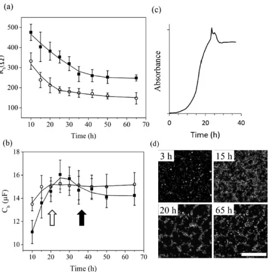
interactions at the electrode surface (right branch) include constant phase element (CPE), anomalous diffusion (Zd) and charge transfer resistance (RCT). Bulk solution resistance is represented by Rs. ... 51 Figure 2.5 Trends of Rb (a) and Cb (b) during templated biofilm growth at the working electrode corner () and middle (). Error bars were produced from the standard deviation of four measurements for each time point. QC/QT = 0.5 and

QC+QT = 1.2 mL·h-1 for all measurements. Arrows mark the times from Figure 3

when exponential growth ends for corner (solid) and middle (hollow). (c) Normalized absorption signal from Amide II band in time for Pseudomonas sp. Visual confirmation of biofilm restructuring at the attachment surface in the channel middle by CLSM (d) after 3 h, 15 h, 20 h, and 65h using 40× objective. Scale bar (100 μm) in image at 65 h is representative of all images. ... 54 Figure 2.6 Flow rate dependency of fitted bioresistance (a) and biocapacitance (b) for 65 h old Pseudomonas sp. biofilm that had been cultured under QTot= 1.2

mL·h-1 with flow rate ratio QC/QT =2. Red data points show the average values

from three separate experiments, with error bands representing the standard deviation in their measurements. Blue triangles show the trend of resistance and capacitance changes with the same flow rates after shear-removal of significant portions of biofilm. Error bars show standard deviation in their measurements. The last point in each plot shows the R and C values after returning the system

cultivation flow rate of 1.2 mL·h-1. (c) Optical micrographs showing typical long-range effects on biofilm due to changing shear forces. (i) Raw image in region of interest obtained at total flow rate Qtot=1.2 mL·h-1. Dashed red circles highlight the optically dense biofilm formations, which produced streamer formation under elevated flow in subsequent images. Background corrected images using (i) for the same region of interest at total flow (ii) Qtot=0.6 mL·h-1, (iii) Qtot=2.4 mL·h-1, (iv) Qtot=3.6 mL·h-1, (v) Qtot=4.8 mL·h-1, (vi) Qtot=6 mL·h-1, (vii) Qtot=1.2 mL·h-1. In all images, flow is from right to left as indicated by the arrow in (ii). A representative scale bar in (vii) is 250 µm. For all data in (a-c) measurements

were obtained 10 min after QTot was changed. Optical density mode images of

biofilm growth at the electrode-containing microchannel surface before (d) and after (e) application of high shear stresses. Pixel intensities were calculated from OD = -log (It/I0), where It was the time varying intensity from a specific pixel and I0 is the intensity of the same pixel in the background image. Scale bar is 500 µm. Flow was from right to left. (f) OD vs. time plot of the biofilm growing in the electrode-containing channel during EIS measurements. Error band was obtained from the standard deviation of the pixel intensity from the 2000×610 µm microscope field of view shown in (d) and (e) at each time. ... 57 Figure 2.7 Cyclic voltammetry of potassium ferricyanide (10 mM) in biofilm growth medium using gold pseudo-reference (black line) and Ag/AgCl, KCl (3 M) reference electrode (dashed line). ... 62 Figure 2.8 Parallelized electrical model to explain the respective reduction and augmentation of resistance and capacitance during biofilm growth. All electrical elements have the same meaning as described in section 2.8.2. ... 64 Figure 2.9 Biofilm-covered area versus time in (a) corner- and (b) middle-templated growth at different times. Red dotted lines show the approximate interface between template and confinement flow. Double-sided arrows show the region of templating. Scale bar in (a) and (b) are 450 µm. ... 64

Figure 2.10 (a) and (b) show, respectively, the corresponding cross-section and bird’s eye views of the channel (same channel dimensions as above) containing an embedded diamond ATR-FTIR sensing element (2mm × 2mm). (a) The anvil with see-through optics (grey) is pressed against a hard transparent plastic plate (orange). Length, height and width were L=33 mm, h=300 µm and w=2 mm, respectively. ... 66 Figure 2.11 CV from analysis of continuous CLSM experiments conducted over a 65 h period following inoculation. CV was calculated from images of bacteria embedded in biofilms adhered to the glass slide of a microfluidic device. Acquisition was conducted using a 40× objective. ... 68 Figure 2.12 Shifting biofilm colonies at the attachment surface. (a) Position of

GFP bacteria under cultivation flow conditions QTot=1.2 mL∙h-1 (green) and after

reaching 6 mL∙h-1

(red). (b) After position of the GFP bacteria after flow rate returns to initial flow conditions QTot=1.2 mL∙h-1 (yellow) compared to original positions before flow was increased (green). The green data in both (a) and (b) are identical. ... 69 Figure 3.1 (a) Schematic of a three-electrode glass-sealed microfluidic flow cell with dimensions 2 mm width, 400 µm height and 30 mm length. The system consists of graphite working (WE) and counter-electrodes (CE) and a gold pseudo-reference electrode (RE). (b) Cross-sectional view of the microchannel with the sealing glass on top (purple) and an electrode on the bottom. Inset (below) shows an SEM image of the G. sulfurreducens biofilm at the downstream edge of the WE acquired after the end of an experiment. (c) Changes to current outputs (I) for biofilms subjected to solutions with [Ac] = 10

mM during modulations of their flow rates to between Q = 0.2 and Q = 1 mL·h-1

(green and red arrows, respectively, shown for the first flow cycle). ... 80 Figure 3.2 (a) CA of G. sulfurreducens during growth with [Ac] = 10 and 0 mM

concentrations and Q = 0.2 mL·h-1. The asterisk highlights the region of applied

times at which CVs were conducted (CV1 and CV2) under modulated Q. (b) CV

of G. sulfurreducens biofilm 6 h after switching to [Ac] = 0 mM (marked CV1 in

(a)) and changing between Q = 0.2 (blue and black) and Q = 1 mL·h-1 (red). The

inset shows baseline subtraction acquired at Q = 0.2 mL·h-1 to clarify the position of the electrochemical redox potentials. Green and orange arrows point

to redox peaks associated with the first and second redox centers (Ef1 and Ef2),

respectively. The positions of Ef1 and Ef2 (green and orange dots, respectively)

were calculated using the arithmetic mean of the reduction and oxidation electrochemical potentials of each redox center. (c) Non-responsive formal potential under same flow rates as in (a) after continuation of starvation conditions for another 16 h (CV2). In both (b) and (c), CVs were collected with scan rate (1 mV·s-1) after a flow stabilization period of 15 min. ... 84 Figure 3.3 (a) CV of an electrode-adhered G. sulfurreducens biofilm exposed to

turnover concentrations, [Ac]tn ([Ac] = 10 mM), with flow rates of Q = 0.2 (black

curve), Q = 1 (red curve) and Q = 5 mL·h-1 (blue curve). Inset shows first-derivative plot used to find the formal potential. (b) CV curves of an electrode-adhered G. sulfurreducens biofilm exposed to nutrient-limited concentrations, [Ac]ltd ([Ac] = 0.3 mM), with flow rates of Q = 0.2 (black), Q = 0.75 (pink) and Q =

2 mL·h-1 (green). CVs of electrode-adhered G. sulfurreducens biofilm exposed to

[Ac]tn acquired with a scan rate of 1 mV·s-1 and exposed to [Ac]ltd with a scan rate of 5 mV·s-1 (for easier identification of redox peaks). The biofilm age for (a) and (b) is 220 h. ... 86 Figure 3.4 (a) Example CVs of G. sulfurreducens used to generate a calibration curve of formal potential at different pHs. Scan rate (5 mV·s-1). Inset: Calibration curve of cytochrome c formal potential as a function of pHs. The error bars resulting from 3 separate experiments are smaller than the data points. (b) Flow rate dependency of ΔpHb under turnover ([Ac]tn = 10 mM) and nutrient-limited

concentrations (and [Ac]ltd = 0.3 mM). Error bars show standard deviation in the

Figure 3.5 Summary of the effects of hydrodynamic cycling on ΔpHb and proposed factors (italics) leading to a higher electrical current from electroactive biofilms in a microchannel. Deacidification is a general term that includes wash out of acidic by-products and increased neutralization by buffer molecules from the nutrient solution. The biofilm is shown protruding into the cross-flow stream from a continuous segment of the microchannel wall consisting of an embedded working electrode and the surrounding PDMS (cross-hatched and orange, respectively). ... 89 Figure 3.6 (a) CVs bulk experiments in 10 mM Ac with Ag/AgCl, 3M KCl (red), a clean Au RE (black), and a Au RE after being used for a 15 day G. sulfurreducens biofilm experiment (blue). (b) First derivative of bulk experiment CVs, which green circles marking the formal potential for the Ag/AgCl and clean Au RE. In each case a shift of E ≈ 410 mV was observed when using different

REs. Therefore, Ef (vs. Ag/AgCl) = Ef (vs. clean Au) – 410 mV and -396 for the

used Au RE. ... 93 Figure 3.7 (a) Stability of the reference electrode measured by CV of ferricyanide in bacterial medium solution at time t=0 (black) and t=2 week (red). (b) Formal potential stability in flow for pH-independent redox reactions of 10 mM ferricyanide. ... 94 Figure 3.8 A three-electrode microfluidic device contained within the anaerobic enclosure with electrical, fluidic and gas connections via feedthroughs in the cap. Insets (i) and (ii) show the microfluidic device outside of the enclosure with red dye to show the channel relative to electrodes and (ii) inside the enclosure during the experiment, respectively. Small discolouration at the WE in inset (ii) is the accumulation of G. sulfurreducens (circled in blue). ... 95 Figure 3.9 (a) Results from a separate experiment during switching from 10 to 0.3 mM acetate (red arrow). Resumption of 10 mM acetate conditions occurred at 460 min (green arrow) after CV measurements. (b) CV after subjecting

t=0 h corresponds to biofilm age of 220 h. Flow rates were Q=0.2 mL·h-1 in both (a) and (b). ... 96 Figure 3.10 Flow rate effects on mature biofilm at 0.2 mL·h-1 (orange arrow) and

1 mL·h-1 (green arrow) for [Ac] = 10 mM (red curve) and [Ac] = 0.3 mM (black

curve). Application of [Ac] = 0 mM with exposure time of 6 h (blue curve) and 24 h (pink curve) with 0.2 mL·h-1 flow rate. ... 97 Figure 3.11 (a) Zoomed view of Figure 1a in main paper of G. sulfurreducens adhered to the WE via SEM using 30 keV, 3000× (scale bar 10 µm). (b) Side-view at an upstream position of the same biofilm shown in main paper Figure 3.1 b. Scale bar is 20 µm, arrow points to exposed graphite electrode at the biofilm base. The measurement of a 60 µm thick biofilm is shown. ... 98 Figure 4.1 Experimental setup. (a) Three-dimensional schematic of a microfluidic electrochemical flow cell showing a gold reference electrode (RE) and graphite working and counter electrodes (WE, CE). Height, width and length were h = 400 µm, w=2000 µm and L = 3 cm, respectively. The exposed working electrode to the channel had the same width as the channel, and extended for 3000 µm along the channel length. The dashed line shows the position of the cross-section for (b). (b) 2D schematic of device cross-section (y-z plane), with three syringe pumps holding gas-tight syringes containing acetate nutrient solutions of 0, 0.2 and 10 mM. The outlet of each syringe was connected to one inlet of a mixing element via a one-way stopcock valve. The mixer outlet was connected to the device inlet. The inoculum syringe is not shown. (c) SEM image of G. sulfurreducens biofilm (>1000 h age) on the working graphite electrode following the experiments described in this work. All experiments were conducted at 22 °C. ... 105 Figure 4.2 The effect of flow and nutrient concentration on current output of a fully mature G. sulfurreducens biofilm. (a) Current profiles due to changes in [Ac]. Region I shows an active biofilm exposed to [Ac] = 200 µM (green). Region II shows a pseudo-active biofilm with exposure to [Ac] = 140 µM acetate (blue).

Region (III) shows an inactive biofilm after exposure to [Ac] = 80 µM (grey). In all cases, QT = 0.5 mL·h-1. (b) Current recorded during increases to acetate

concentration by 10 µM increments below [Ac]PA. Flow rate was QT = 0.5 mL·h-1.

(c) Current output following two separate transitions from inactivity (at [Ac] = 0)

to pseudo-activity via [Ac]PA = 160 µM with QT = 0.25 mL·h-1 (black curve) and

[Ac]PA = 30 µM acetate at QT = 1 mL·h-1 (red curve). (d) Current output following two separate transitions from inactivity to full activity via [Ac]A = 200 µM acetate with 0.25 mL·h-1 flow rate (black line) and [Ac]A = 40 µM acetate with QT = 1

mL·h-1 flow rate (red line). Reduction in current in both data was the result of a

switch to [Ac] = 0 M. ... 107 Figure 4.3 Dependency of concentration thresholds [Ac]PA (hollow circles) and [Ac]A (solid squares) on QT and equivalent flow velocity (vA) for a fully mature biofilm from G. sulfurreducens bacteria. The upper portion of the plot labelled I (white) indicates [Ac], QT conditions resulting in active biofilms. The intermediate band labelled II (blue crosshatch) indicates [Ac], QT conditions resulting in pseudo-active biofilms. And the lower region of the plot labelled III (black

crosshatch) indicated [Ac], QT conditions cause biofilm inactivity. Yellow circles

and the respective trend line (dashed) are the calculated [Ac]f following acetate

consumption at the WE. Error bars were not added as they were smaller than the data points. Inset: Nutrient flux threshold, JA (pmol·s-1), as a function of QT

(red) and maximum current output, Imax (µA), as a function of [Ac]A (blue). Error

bars for all points were generated from three separate experiments at the same flow rate. ... 111 Figure 4.4 Microfluidic electrochemical cell with three-electrode setup and connections inside the anaerobic jar. Flow passes through the micro channel from inlet and touch RE, WE and CE, respectively. Inset: red solution is injected on to the device and withdrawn through connective tubing. The red liquid highlights the microfluidic channel. ... 116 Figure 4.5 (a) G. sulfurreducens biofilm growth in microfluidic channel with 10 mM acetate nutrient and 0.2 mL·h-1 flow rate for 500 h. (b) Reduction of the

current by switching from 10 mM nutrient medium to 0.2 mM Ac nutrient concentration. ... 121 Figure 4.6 CV curve of G. sulfurreducens biofilm on the graphite WE at (a) turnover at 100 h and (b) non-turnover, recorded 5 hours after switching to a nutrient depleted solution. Ef is formal potential of cytochromes C of G. sulfurreducens biofilm. Scan rates were 1 mV·s-1 and 3 mV·s-1 for (a) and (b), respectively. ... 122 Figure 4.7 (a) CA of G. sulfurreducens biofilm profile for approximately the first 200 h hours following biofilm maturation. The red box shows the region of data shown in (b). (c) Nutrient solution was switched to 80 µM acetate medium (blue

arrow) while the flow rate was maintained constant at 0.5 mL·h-1.

G. sulfurreducens biofilm shows a fluctuating (pseudo-active) state after at 80 µm acetate in 40 h exposure time. ... 123

Figure 5.1 Schematic of a 3-electrode glass-sealed electrochemical microfluidic cell with dimensions 2 mm (w) × 0.4 mm (h) × and 30 mm (L). RE, WE and CE represent pseudo reference electrode (gold), the working electrode (graphite) and the counter electrode (graphite), respectively. (a) Top view of the microchannel with the sealing glass on top (violet) with one inlet (next to RE) and one outlet (next to CE). The dark blue part shows PDMS which is used for microchannel fabrication. (b) Side view of microfluidic electrochemical cell. The inlet of microfluidic channel is connected to a glass gas-tight syringe with 10 mM

acetate concentration and 0.2 mL·h-1 flow rate. The G. sulfurreducens cells were

grown on the surface of graphite working electrode. The red box shows SEM image (z-y orientation) of mature G. sulfurreducens biofilm on the graphite electrode. ... 132 Figure 5.2 Flow rate modulation from Q = 0.2 mL·h-1 (base flow) to elevated values, Q = 0.4, 0.6, 0.8, 1, 2 and 3 mL·h-1 for a 600 h old G. sulfurreducens biofilm exposed to [Ac] = 10 mM. Inset: average I vs. Q during for a mature

biofilm (> 600 h) conducted 4 times on four consecutive days. Error bars represent standard deviation of averaged measurements. The blue arrow points to data at Q = 0.2 mL/h that were acquired from background current measurements, whereas the other values were acquired from peak current values in the main figure. The dashed line extrapolates the linear portion of the inset figure to Q = 0 conditions. ... 133 Figure 5.3 (a) Plots of the concentration of acetate nutrient converted for respiration vs. flow rate as a function of the initial acetate concentration. (b)

Plots of P [Ac]i vs. – Ln(1 - P). The modulated flow rates were Q = 0.4 mL·h-1

(pink), 0.6 mL·h-1 (blue), 0.8 mL·h-1 (dark green), 2 mL·h-1 (red) and 3 mL·h-1 (green). (c) Plot of KM(app) vs. Q. The intercept on the vertical axis (red circle) yields a zero-flow KM(app) value ( ) of 0.59 mM. (d) Current vs. initial acetate concentrations in the bulk experiment for 10 mM (black), 7 mM (red), 5 mM (blue), 2 mM (pink), 1 mM (dark green), 0.7 mM (dark blue) and 0.3 mM (purple). The curve was fitted to Eq. 5.4 to find KM(app). Inset: The Lineweaver-Burk plot of the reciprocal current output vs. the reciprocal acetate concentration demonstrates the expected linear profile for systems applicable to Michaelis-Menten kinetics. ... 135 Figure 5.4 Image of the three-electrode device after installation within the anaerobic enclosure. Electrical connections to the counter electrode and working electrode are shown via black and yellow alligator clips. The epoxy-protected solder connection to the gold reference electrode is shown with the white wire. Inset: close up of the microfluidic device before installation and electrical connections with the red dye aqueous solution being passed through the channel for contrast. ... 139 Figure 5.5 The changes of flow rate in function of time of acquisition. The black

lines shows the time in which the flow rate is 0.2 mL·h-1 and blue, purple, green,

Figure 5.6 CV curves of G. sulfurreducens biofilm during growth for 100 h (black curve), 290 h (red curve), 450 h (blue curve) and 540 h (pink curve) after inoculation. ... 144 Figure 5.7 Discharge curves on mature biofilm (540 h growth) at 2 different flow rates and nutrient concentrations following 10 min of charging under OCV conditions. Current acquisition was conducted after switching from OCV to 400 mV vs. Au. ... 145 Figure 5.8 Initial electrochemical growth of G. sulfurreducens. ... 146 Figure 5.9 (a) CA curve of G. sulfurreducens biofilm growth in an electrochemical cell chamber with 10 mM acetate nutrient (WE potential: 0 V vs Ag/AgCl), (b) CA curves of G. sulfurreducens biofilm at different acetate concentrations. The current output from G. sulfurreducens biofilm has been recorded after reaching to steady state conditions for around 90 min. ... 147 Figure 5.10 Changes in device reaction capacity with flow rate, using data from Table 5.1. The blue dotted line extrapolates backwards the trends from the linear portion of the curve to static flow conditions at Q=0. ... 149 Figure 6.1 (a) Initial current versus time plots for reactivation of a mature G.

sulfurreducens biofilm upon switching from [Ac]=0 mM to [Ac]=10 mM (solid

lines) and [Ac]=0.2 mM (dash lines) nutrient solution at Q=0.75 mL·h-1 (black), Q=0.5 mL·h-1 (red), Q= 0.25 mL·h-1 (green). The time t=0 was the time of switching to the Ac containing solution and the delay in the increase to the current was due to the time required for the new solution to reach the biofilm. (b)

Two examples of 0.25 mL·h-1 flow rate in 10 mM acetate nutrient (solid line) and

0.2 mM (dash line) with exponential growth constant (k) values. Red lines shows fitting curves for exponential growth. (c) Trends in the reactivation growth

constant (µA·h-1) vs. Q (mL·h-1) after switching to 20 mM (gray), 10 mM (black),

7 mM (red), 2 mM (blue), 0.85 mM (blue light), 0.7 mM (purple) 0.2 mM (green) from [Ac]=0 mM conditions. Error bars were acquired from at least three

separate experiments and were smaller than the data points in many cases. The dashed lines show linear fit for each data set, which were extrapolated backward to obtain predicted minimum the reactivation growth constant, dI/dtmin (at Q=0) and the minimum flow rate, Qmin, required achieve a biofilm reactivation for [Ac]=0.2 mM. ... 152 Figure 6.2 A schematic of ATR-IR electrochemical cell for which can be used for IR-spectroelectrochemical studies of G. sulfurreducens cells. ... 154 Figure 6.3 A simple proposed set up for DIET studies with different kind of microorganisms. By applying microfluidic tools can have an environment control or inputs and outputs of system for EET investigation. ... 155 Figure 6.4 A simple proposed set up for pili separation from bacteria for DET or DIET studies with different kind of microorganisms. ... 156

List of tables

Table 3.1 Velocities by convection and diffusion (of H+) and shear stress based on typical flow conditions used in this study. ... 92

Table 4.1 Hydrodynamic parameters in the clean portions of the channel (grey) and above the biofilm (orange) for typical flow conditions used in this study. . 119 Table 4.2 Comparison of current fluctuations between active and pseudo-active biofilms. ... 124

Table 5.1. Tabulation of changes to mean proton diffusion velocity ( ̅ ), channel flow velocity ( ̅ ), Reynolds number (Re), shear stress ( ̅), Apparent

Michaelis-Menten constant (Km(app)) and device reaction capacity

List of abbreviations

Attenuated total reflection Bioelectrochemical system Chronoamperometery Biocapacitance

Cytochrome c

Double layer capacitance Counter electrode

Confocal laser scanning microscopy Constant phase element

Cyclic voltammetry Coefficient of variance Direct electron transfer

Direct interspecies electron transfer Electroactive biofilm

Extracellular electron transfer Formal potential

Electrochemical impedance spectroscopy Extracellular polymeric substance

Electron transfer Ferrocene

Green florescence protein Glucose oxidase

Catalytic rate Michaelis constant

Apparent Michaelis constant Lysogeny broth

Microbial 3-electrode cell Microbial desalination cell Microbial electrolysis cell Mediated electron transfer Microbial fuel cell

Optical density

Outer membrane cytochrome c Oxidized form

Poly dimethyl siloxane Bioresistance

Charge transfer resistance Remolds number

Red RS SCE TCA Tg WE Z Z' Z'' Zd Reduced form Solution resistance

Saturated calomel electrode Tricarboxylic acid cycle Glass transition temperature Working electrode

Absolute impedance Real impedance Imaginary impedance

Acknowledgment

First of all, I would like to thank my thesis director, Professor Jesse Greener, for trusting me with this ambitious project and for giving me all the necessary resources for its accomplishment. Professor Greener, with his availability and critical sense, has a big part in the success of this project and working with him was a source of inspiration and motivation for me every day. He has allowed me immeasurable learning in 3 different scientific field (electrochemistry, microbiology and microfluidics) that will allow me to face future challenges.

I would also like to thank my co-director, Professor Steve Charette, for his support and help throughout these years of research. He was a great help to me in microbiology part of this thesis and was a key element in the success of this project. Without him and his generosity in providing and permission of using the microbiological instruments such as anaerobic glove box, these successes were not possible.

I would like to thank all the members of the Chemistry Department as well as the Biochemistry, Microbiology and Bioinformatics Department, especially Rodica Neagu-Plesu, Luc Trudel, Laurent Smith, Véronique Samson and Valérie Paquet who had huge impacts in success of my scientific projects.

My experience would have been incomplete without my colleagues from Greener’s research team. I would like to thank Adnan, François, Eya, Mazeyar, Mohammad, Mehran, Farnaz, Erica, Jia and newcomers: Dirk, Gong and Tanver for making this difficult journey of research a little easier and making the laboratory great. I also want to thank all of summer interns, Arnaud Reitz, Julien, Mahdi, Sabrina, Maxim, Valérie, Germain, Brandon and Kimberly in lab during my research. I passed a great time and I learned several things by exchanging with you.

Finally, I would like to sincerely acknowledge my family. I thank you for your support and unconditional kindness.

Foreword

The following section lists the published works for each chapter including the contribution of each author.

Chapter 2. Zarabadi, M. P., Paquet-Mercier, F., Charette, S. J. and Greener, J. Hydrodynamic Effects on Biofilms at the Biointerface Using a Microfluidic Electrochemical Cell: Case Study of Pseudomonas sp. Langmuir, 2017, 33(8), 2041-2049.

Contribution: M.P.Z., J.G., and S.J.C. formed the concepts of the project and planned the experiments. M.P.Z. fabricated flow channels, made microbiological and bacterial preparations, conducted all electrochemical experiments and analysis and some confocal laser scanning microscopy (CLSM) experiments and analysis. F.P.M. conducted ATR FT-IR and some CLSM experiments and analyzed them. The manuscript writing and editing was mostly done by J.G and M.P.Z. The manuscript was reviewed and edited by S.J.C.

Chapter 3. Zarabadi, M. P., Charette, S. J. and Greener, J. Flow‐Based Deacidification of Geobacter sulfurreducens Biofilms Depends on Nutrient Conditions: a Microfluidic Bioelectrochemical Study. ChemElectroChem, 2018, 5, 3645-3653.

Contribution: M.P.Z., J.G., and S.J.C. formed the concepts of the project and planned the experiments. M.P.Z. fabricated flow channels, made microbiological and bacterial preparations, and conducted all electrochemical experiments and analysis. The manuscript writing and editing was mostly done by J.G. and M.P.Z. The manuscript was reviewed and edited by S.J.C.

Chapter 4. Zarabadi, M. P., Charette, S. J. and Greener, J. Toggling Geobacter

sulfurreducens metabolic state reveals hidden behaviour and expanded

applicability to sustainable energy applications, Sustainable Energy & Fuels, 2019, DOI: 10.1039/C9SE00026G

Contribution: M.P.Z. and J.G. formed the concepts of the project and planned the experiments. M.P.Z. fabricated flow channels, made microbiological and bacterial preparations, and conducted all electrochemical experiments and analysis. The manuscript writing and editing was mostly done by J.G. and M.P.Z. The manuscript was reviewed and edited by S.J.C.

Chapter 5. Zarabadi, M. P., Couture, M., Charette, S. J. and Greener, J. A generalized kinetic framework for whole-cell bioelectrocatalysis in flow reactors clarifies performance enhancements, ChemElectroChem, 2019, 6, 2715-2718. Contribution: M.P.Z. and J.G. formed the concepts of the project and planned the experiments. M.P.Z. fabricated flow channels, made microbiological and bacterial preparations, and conducted all electrochemical experiments and analysis. The manuscript writing and editing was mostly done by J.G. and M.P.Z. The manuscript was reviewed and edited by M. C. and S.J.C.

Introduction

Electrochemistry is the branch of chemistry dealing with the combination of electrical and chemical effects. Among the most important applications, include electrical energy production during chemical reactions and chemical changes caused by applying a known electrical current or potential.1 Other industrial applications include development of electro analytical sensors,2 batteries,3 and fuel cells4 to technologies (the electroplating of metals,5 electrochemical extraction6 and corrosion).7

Bioelectrochemical processes can take place in an electrochemical energy conversion device. Bioelectrochemical systems (BES) include microbial electrolysis cells,8 microbial fuel cells,9 enzymatic biofuel cells10 and microbial electrosynthesis cells.11 Microbial fuel cell (MFC) technology generates electricity from organic compounds that may be sourced from organic waste, through the catalytic activity of microorganisms such as bacteria. In a chemical point of view, the MFC based technology therefore converts the energy stored in chemical bonds of organic compounds to electrical energy, through the catalytic reactions by microorganisms. Microfluidics consists of channels with 10-1000 µm length scale in at least in one dimension. It can be used to accurately manipulate nanoliter sample volumes, making it an interesting technology to scale down and potentially automate culture-based platforms.12 With the ability to run several low cost essays in parallel, microfluidics has the potential to revolutionize the ability to perform procedures such as high-throughput biological and chemical sensing, electrochemical and energetic analysis.

The introduction part of this PhD thesis demonstrates an overall literature review about BESs and microfluidics in the field of biosensing and bioconversion of energy.

Chapter 1. Background

1.1 Electrochemical cell

An electrochemical cell is used to control and monitor electrochemical reactions (a process in which electrons flow between two substances) by the input of

electrochemical signals or create voltage and current from chemical reactions.1

Generally, an electrochemical cell consists of two or three electrodes. Inert conducting materials such as platinum, gold and graphite are examples of typical

electrode materials used in electrochemical cells.1 The electrodes are usually

placed in an electrolyte. Based on the goals of this project, electrochemists can determine the type of electrodes, electrolyte materials and cell structure and configuration for electrochemical measurement or energy applications.

1.1.1 Electrochemical cell configuration

The simplest electrochemical cell uses two electrodes, an anode and a cathode. In an electrochemical cell, the cathode is the electrode where current flows into while the anode is the electrode where the current flows out of. The cell potential is measured between the anode and cathode. Typically, this setup is used with energy storage or conversion devices like batteries, fuel cells and photovoltaic panels.1 A simple equation, power (W) = potential (V) × current (I), gives power output from an electrochemical cell. By measurement of potential difference between anode and cathode, and calculation of current, and therefore cell power will be measurable. The readers refer to the section 1.2.2.2 for more information. The 3-electrode cell setup is the most common electrochemical cell configuration used in electrochemistry. In this case, the current flows between the working electrode (WE) and the counter electrode (CE) and the potential difference between reference electrode (RE) and WE is controlled through a potentiostat.13 This configuration allows the potential of an electrochemical reaction to be controlled, whereas no such control is provided in a 2-electrode setup. A reference

electrode has a stable and well-defined electrochemical potential (at constant temperature) against which the applied or measured potential in an electrochemical cell is referred. Ag/AgCl in saturated KCl and saturated calomel electrodes (SCE) are the most well-known reference electrodes in electrochemistry laboratory.13 In some electrochemical devices, such as miniaturized microfluidic electrochemical cells, it may not be possible to use a standard reference electrode. In such cases, a pseudo-reference electrode, generally a metal such as gold or silver, can be used. The most important challenge for a pseudo-reference electrode is stability and constancy of electrochemical potential during the measurements. This issue is addressed in this thesis.

1.1.2 Electrochemical techniques

Measurements in an electrochemical cell include (1) measuring the potential when the current is zero (potentiometric), (2) measuring the potential while controlling the current (galvanostatic), and (3) measuring the current while controlling the potential (potentiostatic). In galvanostatic measurements, the experiment is carried out by applying the controlled current between the WE and CE with a current source and monitoring the potential between the WE and RE. In a potentiostatic (voltammetry) experiment, a time-dependent potential is applied to a WE and the resulting current is recorded. A plot of current versus potential is called a voltammogram and it is

the electrochemical equivalent of a spectrum in spectroscopy.13

Based on the main goals of this thesis, we only focus on voltammetry mode with three well-known electrochemical techniques. The cyclic voltammetry (CV), chronoamperometery (CA) and electrochemical impedance spectroscopy (EIS) are discussed in the following sections.

1.1.2.1 Cyclic voltammetry (CV)

In a cyclic voltammogram, a scan of electrochemical potential will be completed in both directions of negative and positive potential. Figure 1.1a shows a typical

potential-excitation signal. In this example, we first scan the potential to more negative values, resulting in the following reduction reaction.

Ox + ne- Red (Eq. 1.1)

When the potential reaches a predetermined switching potential, the electrochemical potential sweep direction will be reversed resulting toward more positive potentials. Because the reduced form of the analyte was generated on the forward scan, the reduced form of the analyte will be oxidized during the reverse scan.

Red Ox + ne- (Eq. 1.2)

The resulting cyclic voltammogram provides an opportunity for measurement of the peak currents and peak potentials (Figure 1.1b). The separate peaks of reduction and oxidation reactions can be characterized by a peak potential and a peak current. For a reversible system, the anodic and cathodic peak currents are equal,

and the half-wave potential, E1/2, is midway between the anodic and cathodic peak

potentials which is called formal potential (

). Studies of the electrochemical behaviour of species generated at the surface of the electrode can be carried out with scanning the electrochemical potential in both oxidative and reductive directions.1

Figure 1.1 (a) One cycle of potential scanning showing the initial potential (more positive potential) to the switching potential (more negative potential) and then, coming back to initial potential value. (b) The resulting cyclic voltammogram showing the measurement of the peak currents and peak potentials.

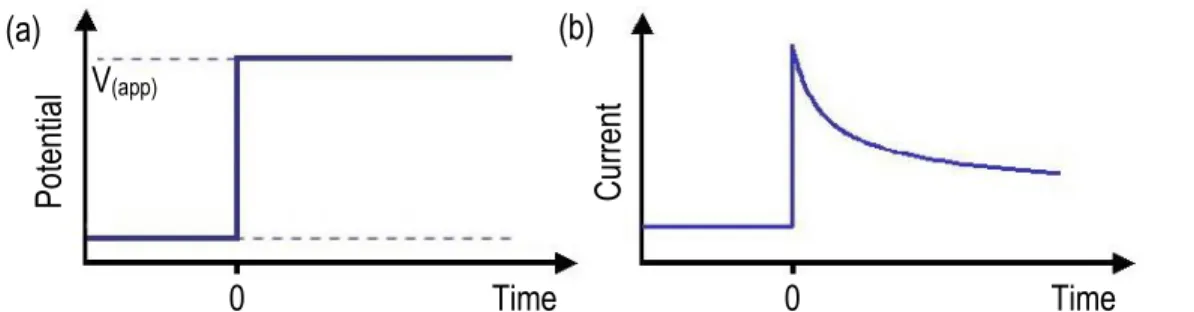
1.1.2.2 Chronoamperometery (CA)

In chronoamperometery, a constant electrochemical potential is applied to the electrode and current as a function of time will be measured. At t = 0 and in presence of redox active species solution, the electrochemical potential is stepped

to a value significantly more negative or positive than the Ef for the redox couple.

Immediately after applying electrochemical potential, the electroactive species in

the vicinity of the electrode are converted to Red or Ox.1 With a known electrode

area, measurement of either stoichiometric number of electrons involved in the reaction or diffusion constant for electroactive species is easily accomplished.

Potential +

-

-

-

Figure 1.2 (a) Potential of the electrode versus time. At t = 0, a constant potential,

V(app), is applied on the electrode and it is maintained constant during

measurement. (b) Curve of chronoamperometery, which shows changes of current versus time.

1.1.2.3 Electrochemical impedance spectroscopy (EIS)

Electrochemical Impedance Spectroscopy (EIS) is a powerful technique for the characterization of electrochemical systems. At an applied electrochemical potential, with a sufficiently broad range of frequencies, the influence of physical and chemical phenomena can be isolated and distinguished. EIS has found widespread applications in the field of characterization of coatings, batteries, fuel cells, materials and corrosion studies.14

The fundamental approach of all impedance methods is to apply a small amplitude sinusoidal potential and measure the response (current or voltage). In a potentiostatic EIS experiment, a small AC amplitude sinusoidal excitation signal (ΔE ∙ sin (ωt)), with a particular frequency ω, is superimposed on the DC polarization potential (E0). As a result, the current response will be (ΔI ∙ sin (ωt+φ)). The impedance of the system can be calculated using Ohm’s law. The ratio of E(ω) to I(ω) results the impedance Z(ω). This impedance of the system is a complex quantity with a magnitude and a phase shift (φ) between the AC potential and the current response, which both depend on ω of the signal. The impedance of the

system can be resulted by sweeping the frequency (typically between 100 KHz –

0.1 Hz) of the applied electrochemical potential.16

0 Po te ntia l Time V(app) (a) 0 C ur re nt Time (b)

EIS results are usually represented by one of two plots. A Nyquist (complex) plot includes 2 parts of real and imaginary impedance. Nyquist representation gives an overview of the data, with the shape of the Z’ (real impedance) vs. Z” (imaginary impedance) curve can make qualitative interpretations, but the frequency is shown. This problem is solved by the Bode plot, where the absolute value of impedance (|Z|) and the phase shifts (φ) are plotted as a function of frequency in two different plots giving a Bode plot. Figure 1.3 shows a typical Nyquist and Bode plot.

Figure 1.3 (a) Typical Nyquist plot based on Randles circuit model. (b) Typical Bode plot based on the same Randles circuit model.

An equivalent electrical circuit model should be used for analysing EIS data output. By fitting EIS data into an appropriate equivalent circuit model, physical electrochemistry parameters of the system can be extracted. As an example, one of the most common cell models is the Randles circuit model.15 It includes a solution resistance (RS), a double layer capacitance (Cdl) and a charge transfer

resistance (RCT) (see Figure 1.4). The charge transfer resistance is in parallel with

the double layer capacitance. This simplified Randel’s cell is the starting point for

other more complex models for biological sensors, energy storage devices, fuel cells and corrosion studies. Figure 1.3 demonstrates an output EIS data, which can be fitted with a Randles circuit model. It should be considered that this is one of the simplest examples of an electrochemical system whereas typically, equivalent

circuits can be much more complex. Based on Randles circuit, the semi-circle shape in Nyquist curve represents charge transfer resistance, therefore by the increasing diameter of the semi-circle curve indicates a higher charge transfer.

Figure 1.4 (a) Randles equivalent circuit (b) Nyquist curve of Randles circuit.

1.2 Bioelectrochemistry

The term “bioelectrochemistry” can be defined as the area of the science that utilizes electrochemical principles and techniques to investigate electrochemical

processes of relevance to biological systems and biomaterials.16

Bioelectrochemistry focuses on the structural organization and electron transfer (ET) functions of biointerfaces on electrode surfaces.17 Applications include the

development of devices such as electrochemical biosensors,18 medical tools,19

biofuel cells and other energetic applications.20 Over the past 20 years,

bioelectrochemistry has been proven to be a useful means to understand the electrochemical properties of biomolecules such as proteins, enzymes, lipids, nucleic acids and even whole cells such as bacteria. Also, it is a powerful tool for

exploitation of biomolecules in biosensors and biofuel cell devices.16

Here, we will summarize some important topics in the field of bioelectrochemistry related to detection of certain analytes (proteins, bacteria and biomass) via various biosensors and also bioenergetic devices such as microbial fuel cells (MFC). This will include a discussion on how electrochemical biosensing occurs between biomass and the electrode surfaces in the case of both electroactive and

non-RS Cdl RCT RS RCT (a) (b)

electroactive species. Moreover, we will discuss the role of bioelectrochemistry in BES for energy applications. This section will finish with a discussion about ET kinetics between electroactive bacteria and the electrode surfaces.

1.2.1 Bioelectrochemical sensing

Development of electrochemical biosensors has grown rapidly over the last two decades. An electrochemical biosensor is generally defined as a transducer, which

converts biological phenomena into quantifiable and processable signals.21

Electrochemical techniques predominantly use functionalized electrodes to

increase analyte selectivity and sensitivity over non-functionalized electrodes.22 In

any case, sensitivity can be improved by selection of right electrochemical

technique such as CV and EIS.23

Figure 1.5 Scheme of an electrochemical biosensor. Biological sensing elements are coupled to working electrode. These traduce the signal to deliver a readable output.

Biological sensing elements

DNA

Cells

Enzymes and proteins

Electrochemical transducer electrodes _{Signal processor}

Readable output

The schematic of a typical electrochemical biosensor is shown in Figure 1.5, which consists of an electrochemical transducer device and a signal processor. The WE (in a 3-electrode configuration) is usually functionalized to increase binding with analytes, usually in solution. The mechanism for immobilization of the functional group(s) on the surface of the electrode and their interactions with the target molecules can change electrochemical properties of the electrode, resulting in a readable output in terms of current, potential, impedance, capacitance, conductance or other electrical parameters.24 However, because of the sensitivity of the electrode surface, surface electrode changing (generally interfacial capacitance) can be used as an electrochemical biosensor for biomass detection, e.g. accumulation of bacteria,25 neurotransmitters26 and glucose.27

In the next section, we give an example for bioelectrochemical sensing based on CV and EIS techniques.

1.2.1.1 Biomolecule sensing with CV and EIS

One of the most well-known examples for electrochemical biosensing devices is the glucose sensor. There are several examples for different types of glucose

sensors with different detection limits and electrochemical techniques.28 The

electrochemical biosensing based on glucose oxidase (GOX) has attracted

widespread interest owing to their importance in glucose monitoring and quantification. Three steps are involved for detection and measurement of glucose

in a system. GOX (Ox) reacts with glucose forming gluconolactone (Eq. 1.3). Then

the reduced form can be re-oxidized by ferrocene (Fc) (Eq.1.4).29 An oxidative electrochemical potential can oxidize Fc to Fc+ (Eq. 1.5) and by measurement of amount of oxidized Fc, the glucose concentration can be calculated.

1) GOX (Ox) + glucose GOX (Red) + gluconolactone (Eq. 1.3) 2) GOX (Red) + 2 Fc+ GOX (Ox) + Fc (Eq. 1.4) 3) Fc Fc+ + e-

Bioelectrochemical devices can be used in immunology, as well.30 Immunosensors are anticipated to be one of the most important types of biosensors, with a wide range of applications in clinical diagnosis, food quality control, environmental

analysis, detection of pathogens or toxins and forensics.31

EIS is another important electrochemical technique used in electrochemical

biosensors.32 In faradiac impedance measurements, the main parameter is the

charge transfer resistance is modified by surface adhered species, usually by products of biochemical reactions. In this approach, a redox probe molecule is added to the analyte solution, which provides a faradaic current when an appropriate potential is applied to the electrode.33 This procedure will be only applied when no electroactive biomolecules present in analyte. The interface blocking by surface products of biochemical reactions can change charge transfer resistance of redox probe molecules and it can be a function of blocking percentage of the surface. It should be considered that redox reactions within biomolecules reactions (electroactive proteins or enzymes) are assigned faradaic possess and can be interpreted with Randels equivalent circuit like redox probe in electrolyte solution.33

When a redox pair is absent from the analyte solution, (neither the presence of a redox probe nor an electroactive biomolecule) the impedance is termed non-faradaic34 and depends on the conductivity of the supporting electrolyte and/or

impedimetric electrode interfacial properties.34 In the absence of a redox pair or if

its charge transfer rate on the electrode is very slow, no faradaic process occurs, and subsequent electron transfer is not produced. In these cases, the interfacial

capacitance changes are often studied.35 The equivalent circuit for this type of EIS

can be represented in different models. The formation of biochemical reaction products may be represented by an additional capacitor and/or resistor based on

EIS is used extensively to follow changes of RCT in electrochemical cells. Blocking the electrode surface with the bulky biomolecules,37 probing with electroactive species, or precipitation of insoluble materials due to the biochemical reactions38 were the main processes observed by faradaic impedance spectroscopy. The changes of interfacial capacitance or resistance based on proposed equivalent model are the main processes in non-faradaic measurements.

1.2.1.2 Electrochemical sensing of planktonic and sessile bacteria

Bacteria can live either as free planktonic cells in bulk solution, or as sessile cells attached to a surface.39 Bacterial biofilms are defined as bacterial populations encased in a protective extracellular polymeric matrix adherent to each other and/or to surfaces or interfaces.40 The biofilm formation is regulated by different genetic and environmental factors. Genetic studies have shown that bacterial motility, cell membrane proteins, extracellular polysaccharides and signalling

molecules play significant roles in biofilm formation, maturation and function.41 The

extracellular polymeric substance (EPS) has a significant role in biofilm formation. They comprise generally, a wide variety of proteins, glycoproteins, glycolipids and in some cases, extracellular DNA.41 A complete biochemical profile of most EPS samples is still a challenge for biochemists.42 The Figure 1.6 shows a general schematic of biofilm structure.

Figure 1.6 A schematic of a generic biofilm and composition of the EPS.

The identification and quantification of planktonic and sessile bacteria and their

biofilms has become a key point in food safety, diagnostics and drug discovery.43

For example, the detection of pathogenic bacteria in planktonic form in water and food samples plays a significant role in early detection for public and environmental

health.44 Generally, electrochemical biosensors are promising for bacterial

detection due to portability, rapidity, sensitivity and ease of miniaturization.45 CV was used to monitor the initial bacterial adhesion as well as subsequent biofilm

maturation stage.46 Like EIS, CV can be done either in presence or in absence of

redox moieties for detection of biomass from bacterial growth. The cyclic voltammograms during bacterial attachment on the surface of the working electrode in an electrolyte solution contained potassium ferricyanide can be changed. As more bacterial cells attach to working electrode, the absolute value of anodic and cathodic currents decreases which confirms reduction of redox reactions of potassium ferricyanide species by blocking the surface of the electrode

with biofilm biomass.47

The reversibility of the electrochemical reaction is observed by difference between the anodic and cathodic peak potentials (∆E), increased with time. These results

Bacteria Proteins DNA Enzymes Polysaccharides Surface