Université de Sherbrooke
Spatialisation du modèle de couvert nival SNOWPACK dans le Nord canadien
pour l’étude de l’accès à la nourriture du caribou de Peary
Félix Ouellet
Mémoire présenté pour l’obtention du grade de Maître ès sciences géographiques (M.Sc.), cheminement de type recherche en géomatique
Juin 2016 © Félix Ouellet, 2016
Directeur de maîtrise :
Alexandre Langlois, professeur au Département de géomatique appliquée, Université de Sherbrooke
Codirecteur de maîtrise :
Alain Royer, professeur au Département de géomatique appliquée, Université de Sherbrooke
Codirectrice de maîtrise :
Cheryl Ann Johnson, Écologiste de la faune, Sciences et technologie du paysage, Environnement et Changement climatique Canada
Membre interne :
Richard Fournier, Professeur au Département de géomatique appliquée, Université de Sherbrooke
Membre externe :
Ludovic Brucker, Earth scientist, Cryospheric Sciences Laboratory, NASA Goddard Space Flight Center
Table des matières
Liste des figures du mémoire ... iii
Liste des figures de l’article scientifique ... iv
Liste des tableaux du mémoire ... v
Liste des tableaux de l’article scientifique ... v
Liste des annexes ... v
Glossaire ... vi
Remerciements ... vii
1. Introduction ... 1
1.1. État de la question ... 1
1.2. Objectifs et hypothèses ... 5
2. Cadre théorique sur SNOWPACK ... 6
2.1. Physique impliquée ... 6 2.2. Entrées ... 7 2.3. Sorties ... 8 2.4. MeteoIO ... 9 2.5. Sngui ... 10 3. Article scientifique ... 12 1.0. Introduction ... 15 2.0. Background ... 17 2.1. Rangifer Tarandus ... 17 2.2. SNOWPACK ... 18
3.0. Data & Methods ... 19
3.1. Study Area ... 19
3.2. Data ... 19
3.3. SNOWPACK Spatialization ... 22
4.0. Results & their Interpretation ... 25
4.1. Preliminary Evaluations ... 25
4.2. Snow Parameters of Interest ... 26
4.3. Software & Operational Results ... 27
4.4. Spatiotemporal Analysis of Grazing Conditions ... 28
4.5. Preliminary Upscaling Approach ... 31
5.0. Discussion & Conclusion ... 32
6.0. Acknowledgements ... 33
4. Éléments complémentaires de méthodologie, de résultats et de discussion ... 38
4.1. Site d’étude ... 38
4.2. Données météorologiques ... 39
4.3. Spatialisation de SNOWPACK ... 41
5. Conclusion globale du mémoire ... 59
Liste des figures du mémoire
Figure 1 : Tendance de température 1950-2014 (source : Goddard Institute for Space Studies,
2015)... 1
Figure 2 : Tendance 1979-2009 (en jours/décennie) de la pluie-sur-neige en Arctique (source : Liston et Hiemstra, 2011) ... 2
Figure 3 : Couches de neige très dure positionnées par rapport à l’épaisseur du couvert nival en région subarctique (source : Johansson et al., 2011). ... 3
Figure 4 : Accès à la nourriture au sol bloqué par la présence de neige dense dans le couvert nival pour le caribou de Peary (vulgarisation). ... 4
Figure 5 : Aspect spatialisation (principe). Pour cet exemple, une information disponible pour un pixel de 5 km x 5 km est spatialisée sur une superficie d’environ 1500 km². ... 5
Figure 6 : Physique impliquée dans SNOWPACK (source : documentation de SNOWPACK). .... 7
Figure 7 : Composantes principales de MeteoIO. ... 10
Figure 8 : Exemple de visualisation sous Sngui (épaisseur de neige et densité dans le temps, péninsule Boothia, hiver 1988-1989 ; inclut le détail quantitatif de la densité pour le 23 mars 1989 à midi). ... 11
Figure 9 : Site d’étude. ... 38
Figure 10 : Organigramme méthodologique global. ... 42
Figure 11 : Organigramme méthodologique (détail du 1er objectif). ... 43
Figure 12 : Organigramme méthodologique (détail du 2ème objectif). ... 44
Figure 13 : Organigramme méthodologique (détail du 3ème objectif). ... 45
Figure 14 : Température de l’air (K) dans le temps : comparaison MRCC vs données mesurées aux stations d’Environnement et Changement climatique Canada à Resolute Bay et du CARTEL (UdeS) à Cambridge Bay. ... 47
Figure 15 : Rayonnement de grande et courte longueurs d’onde descendantes de surface (W/m²) dans le temps : comparaison MRCC vs données mesurées à la station du CARTEL (UdeS) à Cambridge Bay. ... 47
Figure 16 : Comptes insulaires de caribous vs épaisseur cumulée (cm) pour seuil de 400 kg/m³ (Lucie Portier, ex-membre du GRIMP). ... 51
Figure 17 : Indicateur de comptes insulaires de caribous vs indicateur neige (épaisseur cumulée & type de grain) pour tout l’hiver pour un seuil de 300 kg/m³. Les cercles vides représentent les années pour lesquelles aucune couche à aucun moment n’a atteint le seuil de densité. ... 52 Figure 18 : Maxima de l’indicateur de comptes insulaires de caribous par intervalles de
l’indicateur neige (épaisseur cumulée & type de grain) pour tout l’hiver pour un seuil de 300 kg/m³. ... 53 Figure 19 : Exemple de paramétrisation initiale sous Matlab pour la spatialisation... 55 Figure 20 : Écran d’accueil au lancement d’une spatialisation, et étapes impliquées. ... 56 Figure 21 : Polygones associés à la base de données des pixels MRCC (zone d’étude en bleu). .. 57 Figure 22 : Unités désignables pour le caribou (Rangifer tarandus) au Canada (source :
COSEPAC, 2011). ... 65 Figure 23 : Caribou de Peary (source : Environnement et Changement climatique Canada, 2014).
... 65 Figure 24 : Prototype de spatialisation (à gauche, rendu du shapefile ; à droite, rendu matriciel
associé pour la densité en date du 16 mars 2010 à 06h00). ... 67 Figure 25 : Structure des fichiers de profils de neige. ... 68 Figure 26 : Aperçu de la structure de la base de données ponctuelle shapefile des pixels MRCC.
... 68 Figure 27 : Aperçu de la structure de l’extrant principal shapefile (exemple pour l’année 2011). 68 Figure 28 : Comptes insulaires de caribous vs épaisseur cumulée (cm) pour seuil de 325 kg/m³. 71 Figure 29 : Rendu matriciel à partir des données NARR pour l’épaisseur cumulée, la hauteur
totale de neige, un paramètre de fonte / gel et pour le SWE, moyennés de 2000 à 2013. ... 72
Liste des figures de l’article scientifique
Figure 1. Study area. ...19 Figure 2. Cumulative thickness calculation example (threshold of 300 kgm-3). Snow layers’
colours go along with associated density. ...24 Figure 3. Peary caribou island counts in comparison with cumulative thickness (cm) above 300
kgm-3 for all winter seasons (October to May) preceding caribou observations; (a) all counts are shown (unfilled circles represent years where no layers reached the density threshold for the associated location); (b) maximum counts for each 2500 cm cumulative thickness
intervals are shown (data gaps were filled with mean count between preceding / subsequent cumulative thickness intervals). The power relationship plotted has an R² of 0.45. The
bootstrapped standard errors are also shown (based on 5000 iterations). ...26
Figure 4. Raster output result of cumulative thickness (cm) above 300 kgm-3 for all 2011 winter (October to May). Cumulative thickness is presented on a logarithmic scale. Glaciers are not masked, but they were not used in the spatiotemporal analysis presented in Section 4.4. ...28
Figure 5. Preliminary spatiotemporal analysis: cumulative thickness over and under 7000 cm for whole winter, averaged over 5-yr periods. ...29
Figure 6. Preliminary upscaling approach: slope at different spatial resolutions (under / over 1°) for Banks Island. ...31
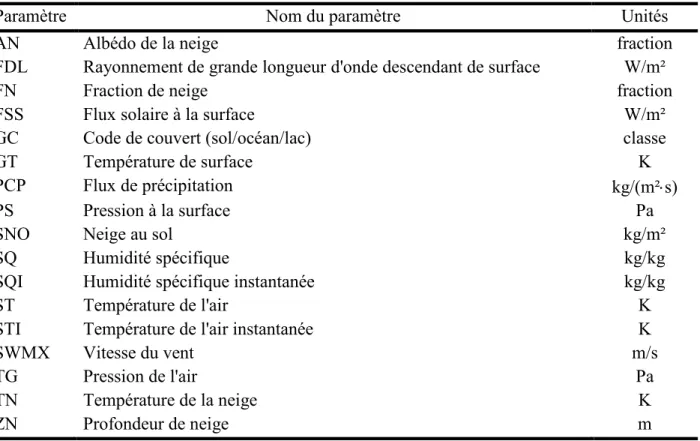
Liste des tableaux du mémoire Tableau 1 : Paramètres météorologiques de SNOWPACK. ... 8
Tableau 2 : Paramètres MRCC disponibles. ... 39
Tableau 3 : Paramètres MRCC vs SNOWPACK. ... 40
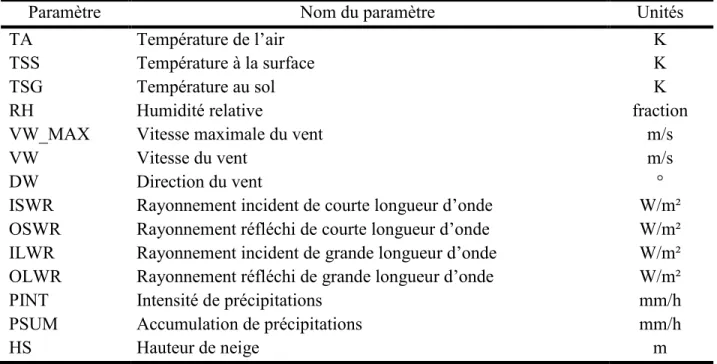
Tableau 4 : Paramètres météorologiques du format SMET. ... 40
Tableau 5 : Paramètres MCanCR4 vs SNOWPACK. ... 69
Tableau 6 : Paramètres NARR vs SNOWPACK. ... 70
Liste des tableaux de l’article scientifique Table 1. The number of Peary caribou surveys per island with corresponding years. ...20
Liste des annexes Annexe 1 – Le caribou au Canada ... 65
Annexe 2 – Choix du modèle de simulation du couvert nival ... 66
Annexe 3 – Prototype de spatialisation ... 67
Annexe 4 – Aperçu des bases de données impliquées ... 68
Annexe 5 – Inclusion des données MCanCR4 ... 69
Glossaire
L’expression couvert nival sera utilisée dans ce document. À noter qu’on aurait pu utiliser l’expression couvert de neige ou couvert neigeux à la place, qui sont des expressions ayant le même sens. On retrouvera aussi l’expression manteau neigeux dans la littérature.
En anglais le terme utilisé est snowpack, qui a inspiré un modèle de caractérisation de couvert nival du même nom, SNOWPACK, qui sera discuté dans le présent document. On peut distinguer l’un de l’autre avec les lettres majuscules. L’expression snow cover sera aussi utilisée. Wikipédia nous donne faussement l’expression accumulation annuelle de neige comme traduction de la page sur le terme snowpack. On comprendra que l’expression accumulation annuelle de neige réfère plutôt à la quantité de neige tombée au cours d’une année, ce qui est différent du couvert nival.
Remerciements
Merci en tout premier lieu à mon directeur de maîtrise Alexandre Langlois, pour son guidage, ses idées, son support et sa disponibilité tout au long de la maîtrise.
Un immense merci à Environnement et Changement climatique Canada, l’initiateur du projet, non seulement pour le financement, mais pour l’étroite collaboration tout au long du projet ; particulièrement merci à Cheryl Ann Johnson (co-directrice) et à Agnes Richards.
Merci à Alain Royer (co-directeur) pour ses judicieux conseils lors de la rédaction des documents au cours de la maîtrise.
Un gros merci aussi aux collaborateurs étudiants / professionnels de recherche au département : Jean-Benoît Madore, Lucie Portier et Roxanne Lanoix.
1. Introduction
1.1. État de la question
En Arctique, la communauté scientifique constate le phénomène des changements climatiques depuis plus de trois décennies (Screen et Simmonds, 2010). Dans cette vaste région nordique, un réchauffement global de 1,06 °C par décennie est observé (Solomon et al., 2007), par rapport à 0,24 °C par décennie pour le Canada (Environnement Canada, 2015). La Figure 1 montre la répartition spatiale de la tendance de température entre 1950 et 2014 et permet de voir le réchauffement accru en Arctique par rapport au reste du globe.
Figure 1 : Tendance de température 1950-2014 (source : Goddard Institute for Space Studies de la NASA, 2015).
Les impacts physiques de ce réchauffement sont multiples, parmi lesquels on dénote des patrons d’anomalies négatives du couvert nival (Derksen et Brown, 2012), de l’étendue de la glace de mer (Stroeve et al., 2011), des glaciers (Gardner et al., 2013) et du pergélisol (Romanovsky et al., 2010). Ces effets ont un impact important sur la réponse de la cryosphère aux changements climatiques, notamment au niveau de l’albédo et de la conductivité thermique de la neige. En effet, via son fort albédo, et sa faible conductivité thermique, la neige conditionne la quantité d’énergie absorbée par la surface (date de fonte des glaciers, du pergélisol, etc.).
Particulièrement pour le couvert nival, qui couvre l’entièreté du territoire arctique en saison hivernale, on observe une fonte plus précoce lors de la saison printanière (Derksen et Brown, 2012).
Le réchauffement actuellement observé amène aussi l’augmentation de l’occurrence d’évènements extrêmes hivernaux tels des vagues de chaleur, des précipitations extrêmes et des périodes de pluie-sur-neige (Callaghan et Johansson, 2011 ; Dolant et al., 2015). Avec le réchauffement actuellement observé, on note une recrudescence de ces évènements dans l’hémisphère nord, dont en Arctique. Par exemple, Liston et Hiemstra (2011) ont démontré l’augmentation de l’occurrence de ces évènements en Arctique entre 1979 et 2009 (la Figure 2 illustre la tendance pour la pluie-sur-neige en jours/décennie), alors que Vincent et Mekis (2006) suggèrent une augmentation de la proportion de précipitations liquides à l’échelle annuelle entre 1950 et 2003.
Figure 2 : Tendance 1979-2009 (en jours/décennie) de la pluie-sur-neige en Arctique (source : Liston et Hiemstra, 2011)
Encore très peu d’études se sont attardées à cette problématique qui amène la formation de croûtes de neige de haute densité (glace, couche de regel, neige croûtée) de plus en plus fréquentes. Parmi ces peu nombreuses recherches, Johansson et al. (2011) ont relevé qu’en région subarctique suédoise, sur une plage d’étude allant de 1960 à 2009, la période la plus récente, soit 1993-2009, est celle présentant le plus de couches de neige très dure, phénomène que l’on peut observer à la Figure 3.
Figure 3 : Couches de neige très dure positionnées par rapport à l’épaisseur du couvert nival en région subarctique (source : Johansson et al., 2011).
L’effet de ces croûtes reste peu connu (Montpetit et al., 2013), mais des études récentes démontrent le potentiel de leur détection avec des outils de télédétection (Montpetit, 2015 ; Dolant et al., 2015). Ceci s’avère intéressant dans la mesure où la présence de ces croûtes, non seulement modifie le bilan d’énergie de surface (Weismüller et al., 2011), mais aussi conditionne l’accès à la nourriture de plusieurs ongulés (Putkonen et Roe, 2003), comme le caribou de Peary.
Le Registre public des espèces en péril du Canada a catégorisé le caribou de Peary, l’unité désignable de l’espèce caribou ayant son habitat dans l’archipel arctique canadien (voir l’Annexe 1 pour son habitat et une image), comme « espèce en voie de disparition ». De façon quantitative, le nombre de caribous de Peary a diminué de plus de 70 % au cours des trois dernières générations (COSEPAC, 2011). Le Registre indique que ces couches de glace ou de neige épaisse et dense constituent le facteur le plus menaçant pour la survie à moyen / long terme du caribou de Peary. En effet, ces couches rendent difficile à certains moments de l’année l’accès à la nourriture au sol, déjà limitée en quantité, pour le caribou de Peary. Cette problématique est illustrée de façon très vulgarisée à la Figure 4.
Figure 4 : Accès à la nourriture au sol bloqué par la présence de neige dense dans le couvert nival pour le caribou de Peary (vulgarisation).
Toutefois, jusqu’à maintenant, la possibilité de quantifier la magnitude de l’effet de ces couches sur les populations de caribous a été freinée par le manque de données caractérisant spatialement les couches en question, l’information étant actuellement accessible localement seulement. Par rapport au manque de nourriture, l’année a été divisée par Environnement et Changement climatique Canada selon trois périodes critiques : la période de mise bas et de migration printanière (avril – juin), celle d’abondance de nourriture et de rut (juillet – octobre) et celle de migration automnale et de survie des jeunes caribous (novembre – mars).
Dans le cadre d’une étude scientifique globale d’Environnement et Changement climatique Canada sur l’avenir du caribou de Peary (incluant la répartition spatiale de la nourriture et des glaces de mer ainsi que la prédation par le loup), le projet de recherche présenté dans ce document se concentre sur la détermination et la mise en place d’un outil de caractérisation du couvert nival ciblé pour l’analyse de l’accès à la nourriture au sol pour le caribou de Peary. On s’intéressera donc aux variations de comptes de caribous causées par la difficulté, voire l’impossibilité, d’atteindre la nourriture se trouvant au sol à travers le couvert nival durant l’hiver.
Ce mémoire est présenté sous forme d’article scientifique qui couvre la méthodologie et les résultats de notre recherche. On rappelle ci-dessous les objectifs et hypothèses du projet (section 1.2) et on présente le cadre théorique à la section 2. L’article scientifique est présenté à la section 3 ; tout ce qui est dans cette section ne sera donc pas repris ailleurs dans le présent mémoire. À la suite de l’article, on retrouve des sections complémentaires, traitant de points qui n’ont pas été soulevés dans l’article, dont une conclusion générale sur le projet de recherche.
1.2. Objectifs et hypothèses 1.2.1. Objectifs
Pour mettre en place un outil d’analyse du couvert nival dans l’archipel arctique canadien (AAC), l’objectif principal du projet est de spatialiser à une échelle régionale la caractérisation locale du couvert nival obtenue avec le modèle de neige SNOWPACK. Le principe de cet objectif principal est illustré à la Figure 5, où l’on peut voir une transition entre une information d’échelle locale et une information spatialisée d’échelle régionale.
Figure 5 : Aspect spatialisation (principe). Pour cet exemple, une information disponible pour un pixel de 5 km x 5 km est spatialisée sur une superficie d’environ 1500 km².
En fait le système doit pouvoir cibler les paramètres du couvert nival directement en lien avec l’accès à la nourriture du caribou de Peary et par conséquent le projet s’articule autour de trois objectifs spécifiques :
1) Pilotage du modèle SNOWPACK à partir d’un modèle climatique
Tout d’abord, le premier objectif spécifique est d’établir une procédure pour piloter le modèle de neige SNOWPACK à partir des données climatiques issues du modèle météorologique MRCC (voir section 4.2) dans l’archipel arctique canadien.
2) Étude et validation des paramètres d’intérêt pour l’accès à la nourriture du caribou de Peary Le deuxième objectif spécifique est d’identifier une relation variable nivale / compte de caribou, la variable nivale étant issue des simulations SNOWPACK pilotées par le MRCC (objectif spécifique 1). Le but est d’établir des liens entre des paramètres nivaux d’intérêt et des données de comptes de caribous, pour ensuite valider ces paramètres d’intérêt à l’aide de mesures terrain.
3) Spatialisation des paramètres d’intérêt et projections futures
Enfin, le troisième objectif spécifique est de spatialiser les paramètres d’intérêt retenus à l’échelle de l’archipel arctique canadien en établissant une procédure automatisée de production de fichiers vectoriels sous format shapefile pour 4 périodes distinctes générées par le MRCC : passé (1980-1985), présent (2010-2015), futur proche (2045-2050) et futur lointain (2090-2095).
1.2.2. Hypothèses
Par rapport à ces objectifs, deux hypothèses ont été identifiées. Pour le premier objectif spécifique, nous avons supposé que la modélisation du couvert nival avec l’outil SNOWPACK allait permettre de simuler des paramètres du couvert nival pouvant être statistiquement liés aux variations de comptes de caribous.
Nous faisons aussi l’hypothèse que des densités élevées de neige pendant la saison hivernale nuisent de façon importante au caribou de Peary (Environnement Canada, 2014), et que cette nuisance se traduit par une réduction du nombre de caribous observés l’été suivant (Gunn et al., 2006).
2. Cadre théorique sur SNOWPACK
SNOWPACK (version 3.3.0 utilisée) est le modèle de simulation du couvert nival retenu (Bartelt et Lehning, 2002 ; Lehning et al., 2002a, 2002b). L’Annexe 2 met en avant-plan les critères qui ont orienté la sélection du modèle. SNOWPACK est un modèle développé par l’Institut pour l'étude de la neige et des avalanches de Suisse (en allemand SLF), situé à Davos, qui fait partie du WSL (L'Institut fédéral de recherche sur la forêt, la neige et le paysage), localisé à Bimensdorf, Bellinzone, Lausanne et Sion.
2.1. Physique impliquée
La physique impliquée dans SNOWPACK est résumée à la Figure 6 ; on peut y voir de façon très synthétisée les processus inclus au niveau du sol, de la neige et de la canopée. Mentionnons à ce sujet plus particulièrement que SNOWPACK peut tenir compte en option de la redistribution par le vent par la création de « pentes virtuelles » consistant en une division du pixel d’intérêt en sous-pixels (jusqu’à neuf sous-sous-pixels). Mentionnons de plus que SNOWPACK peut tenir compte en option de la canopée en insérant entre autres des paramètres locaux de hauteur de canopée et d’indice de surface foliaire. SNOWPACK offre aussi de paramétrer une panoplie d’autres
processus physiques, notamment au niveau de la détection du givre, du transport de l’eau dans la neige / dans le sol et de la détection d’herbe sous la neige.
Figure 6 : Physique impliquée dans SNOWPACK (source : documentation de SNOWPACK). 2.2. Entrées
Le fichier de paramètres d’initialisation ou de configuration (*.ini) comprend l’information sur l’emplacement des deux autres fichiers nécessaires en entrée à SNOWPACK, soit les fichiers d’occupation du sol (*.sno) et de données météorologiques (*.smet), ainsi qu’un éventail de paramètres pour le lancement de SNOWPACK (principalement sur la physique impliquée). Ce fichier d’initialisation peut être créé avec le module INIshell ou à l’aide d’un logiciel de traitement de texte tel que Bloc-notes.
Le format SMET (associé aux fichiers de données météorologiques *.smet) est un format texte comprenant un en-tête ainsi qu’une section de données. L’en-tête comprend entre autres les informations de latitude (ou coordonnée y), de longitude (ou coordonnée x), d’altitude, de projection et les noms des champs. On retrouve la liste des paramètres météorologiques possibles
pour le format SMET au Tableau 4 (section 4.2). Au Tableau 1 on retrouve les paramètres SMET nécessaires en intrant à SNOWPACK.
Tableau 1 : Paramètres météorologiques de SNOWPACK.
Paramètre SMET Nécessaire ? Unités
TA (température de l'air) X K
RH (humidité relative) X %
VW (vitesse du vent) X m/s
ISWR (rayonnement incident de courte longueur d’onde) ou
OSWR (rayonnement réfléchi de courte longueur d’onde) X
W/m² W/m² ILWR (rayonnement incident de grande longueur d’onde) ou
TSS (température à la surface) X W/m² K PSUM (précipitations) ou HS (hauteur de neige) X kg/m² m TSG (température au sol) – K
TS1, TS2, … (températures de la neige à différentes profondeurs) – K Ultimement, SNOWPACK nécessite une commande DOS comprenant :
- la date de fin de la simulation, sous format Année / Mois / Jour / Heure / Minutes - l’emplacement du fichier d’initialisation (*.ini)
- le mode de la simulation (opérationnel ou recherche)
- en mode opérationnel, le nom des stations, séparées par des virgules
2.3. Sorties
Les deux fichiers principaux en sortie de SNOWPACK sont les fichiers *.pro et *.met. Le fichier *.met donne de l’information sur la météo et est donc étroitement lié aux données de météo en entrée à SNOWPACK. Il comprend aussi les données intégrées sur toute la hauteur du couvert nival tels l’épaisseur et l’équivalent en eau. Pour sa part le fichier *.pro est un fichier de profil vertical du couvert nival. Il contiendra les paramètres géophysiques d’intérêt pour l’analyse de l’accès à la nourriture du caribou de Peary. C’est à partir de ce fichier qu’on pourra aussi visualiser le résultat des simulations avec l’outil Sngui présenté à la section 2.5.
Comme SNOWPACK a été développé dans un contexte de simulation de stabilité pour la prédiction d’avalanches, il produit aussi plusieurs indices de fractures potentielles, de résistance et de cohésion entre les couches. Ces paramètres ne sont évidemment pas évalués dans ce travail.
2.4. MeteoIO
MeteoIO (version 2.5.0 utilisée) est une librairie de fonctions qui facilite et sécurise l’accès aux données pour des simulations numériques dans le cadre des sciences environnementales nécessitant des données météo. Dans le contexte du présent projet de recherche, MeteoIO est appelé par SNOWPACK, notamment au moment d’aller chercher les données et de les formater. De manière générale, MeteoIO permet entre autres l’interpolation spatiale et temporelle, le filtrage et le rééchantillonnage de données météo. Il offre une grande souplesse, car il permet de modifier indépendamment les éléments de la librairie. Ultimement, MeteoIO permet une structure sécuritaire en sortie.
Au total, MeteoIO peut faire le pont vers 19 plugins, dont SNOWPACK. Les autres sont, notamment, le format raster d’ArcGIS, le format netCDF, le format SMET et les fichiers météo d’Alpine3D. Le noyau de MeteoIO comprend les éléments suivants :
- API utilisateur - IOManager - IOHandler
- BufferedIOHandler - IOInterface
De façon très synthétisée, IOManager est le point central de MeteoIO, faisant le lien entre l’API utilisateur, IOHandler et BufferedIOHandler. Le lien avec les données météo et les plugins précédemment évoqués se fait via IOHandler, en passant par IOInterface. Au besoin, lors d’une requête sous la forme d’une zone tampon, on passera par BufferedIOHandler. Ensuite viennent se greffer à ces éléments centraux des outils d’interpolation / rééchantillonnage, de configuration, de MNT et autres. On peut voir à la Figure 7 un schéma simplifié du fonctionnement de MeteoIO.
Figure 7 : Composantes principales de MeteoIO. 2.5. Sngui
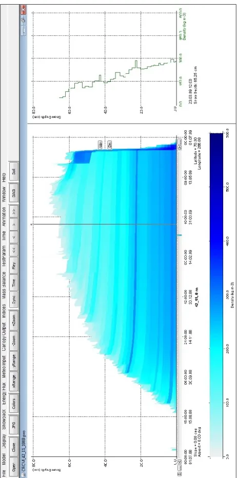
Sngui (aussi nommé en anglais Visualisation of the SNOWPACK model) est un outil de visualisation du fichier de profil de neige (*.pro) en sortie de SNOWPACK ; la version 8.2 (lancée en 2008) a été utilisée. Sngui est inclus dans la version 2 de SNOWPACK, mais a été laissé de côté dans la version 3. Il permet notamment de valider d’un coup d’œil le fichier de profil de neige et d’en faire des analyses primaires. Sous Sngui, on peut visualiser le profil vertical et l’évolution temporelle de plusieurs paramètres du couvert nival, notamment au niveau de la microstructure (grains, densité, résistance) et de l’énergie (chaleur latente, chaleur sensible, gradient de température). Sngui permet aussi à l’utilisateur d’avoir une représentation des paramètres météo en entrée à SNOWPACK. Plusieurs de ces rendus ont servi à l’analyse du couvert nival dans le présent projet de recherche. Un exemple de rendu visuel est illustré à la Figure 8 ; en l’occurrence pour le paramètre de densité de la neige à différentes profondeurs selon le moment de l’année.
Figure 8 : Exemple de visualisation sous Sngui (épaisseur de neige et densité dans le temps, péninsule Boothia, hiver 1988-1989 ; inclut le détail quantitatif de la densité pour le 23 mars 1989 à midi).
3. Article scientifique
L’article scientifique qui suit, qui est donc le point central du présent mémoire, a été soumis à la revue scientifique Physical Geography (éditeur international Taylor & Francis) le 25 novembre 2015. Il est présenté de façon intégrale, et ce seulement en anglais. Il a été écrit en collaboration étroite avec Environnement et Changement climatique Canada. L’article est présentement en révision et devrait être publié prochainement, potentiellement dans une édition spéciale de la revue dédiée à l’événement Eastern Snow Conference 2015, tenu à Sherbrooke en juin 2015, durant lequel le projet a été présenté (Ouellet et al., 2015).
Il est à préciser que la numérotation des lignes, des sections, des figures, tableaux et équations est indépendante au reste du mémoire. Précisons aussi que les références à la section 7.0 de cet article ne sont pas répétées à la bibliographie générale du présent mémoire.
La référence pouvant être utilisée pour citer cet article est la suivante :
Ouellet, F., Langlois, A., Blukacz-Richards, E. A., Johnson, C. A., Royer, A., Neave, E. and Larter, N. C. 2015. Spatialization of the SNOWPACK Snow Model for the Canadian Arctic to Assess Peary Caribou Winter Grazing Conditions. Physical Geography. Submitted, TPHY-2015-0077.
Spatialization of the SNOWPACK Snow Model for the Canadian
1
Arctic to Assess Peary Caribou Winter Grazing Conditions
2
Ouellet, F.1,2*, Langlois, A.1,2, Blukacz-Richards, E. A.3, Johnson, C. A.4, Royer, A.1,2 Neave, E.4 3
and Larter, N. C.5 4
5
1 Groupe de Recherche Interdisciplinaire sur les Milieux Polaires (GRIMP), Université de 6
Sherbrooke, Sherbrooke, QC, Canada. 7
2 Centre d’Études Nordiques, Québec, QC, Canada. 8
3 Water Research Division, Environment and Climate Change Canada, Toronto, ON, Canada. 9
4 Landscape Science and Technology, Environment and Climate Change Canada, Ottawa, ON, 10
Canada. 11
5 Department of Environment and Natural Resources, Government of the Northwest Territories, 12
Fort Simpson, NT, Canada. 13
Spatialization of the SNOWPACK Snow Model for the Canadian
14
Arctic to Assess Peary Caribou Winter Grazing Conditions
15
Abstract
16
Peary caribou is the northernmost designatable unit for caribou species, and its population 17
declined by about 70% over the last three generations. The Committee on the Status of 18
Endangered Wildlife in Canada (COSEWIC) identified difficult grazing conditions through 19
the snow cover as being the most significant factor contributing to this decline. This study 20
focuses on a spatially-explicit assessment tool using snow model simulations (Swiss 21
SNOWPACK modeldriven in an off-line mode by spatialized meteorological forcing data 22
generated by the Canadian Regional Climate Model) to characterize snow conditions for 23
Peary caribou grazing in the Canadian Arctic. The life cycle of Peary caribou has been 24
subdivided into three critical periods: summer foraging and fall breeding (July – October), 25
winter foraging (November – March) and spring calving (April – June). Winter snow 26
conditions are analysed and snow simulations compared to Peary caribou island counts to 27
identify a snow parameter that could potentially act as a proxy for grazing conditions and 28
explain fluctuations in Peary caribou numbers. This analysis concludes that caribou counts 29
are affected by simulated snow density values above 300 kgm-3. A software tool mapping 30
possibly favourable and unfavourable grazing conditions based on snow is proposed at a 31
regional scale across the Canadian Arctic Archipelago. Specific output examples are given 32
to show the utility of the tool, mapping pixels with cumulative snow thickness above densities 33
of 300 kgm-3, where cumulative thicknesses above 7000 cm are considered unfavourable. 34
Keywords: snow; caribou; grazing conditions; Arctic; climate change impacts 35
1.0. Introduction
36
Climate change has been observed in the Arctic over the last four decades (Screen & Simmonds, 37
2010), where an average warming of 1.06 °C per decade has been measured (Solomon et al., 38
2007) compared to 0.43 °C per decade for the rest of the planet (Jin & Dickinson, 2002). 39
Associated physical impacts include negative anomalies in permafrost (Romanovsky, Smith, & 40
Christiansen, 2010), glacier mass balance (Gardner et al., 2013), sea ice (Stroeve et al., 2011) and 41
snow cover (Derksen & Brown, 2012). These trends have an important impact on how the 42
cryosphere responds to climate change, for which snow albedo and thermal conductivity are 43
dominant processes. Snow controls the amount of energy absorbed at the surface of the Arctic 44
Tundra (melt dates for glaciers, permafrost, etc.) through its strong albedo and its low thermal 45
conductivity. 46
The various consequences for snow cover include enhanced spring melting (Derksen & 47
Brown, 2012), winter heat waves, extreme precipitation events, wind and rain-on-snow 48
(Callaghan & Johansson, 2011). It is predicted that these events will become more frequent in the 49
northern hemisphere, including the Arctic, based on current climate warming trends (Liston & 50
Hiemstra, 2011). Few studies have examined how changes in climate affect the formation of 51
dense snow layers and ice crusts. Recent studies have shown the potential for the detection of 52
high density snow layers using satellite remote sensing (Montpetit, 2015). 53
Our growing understanding of snow high-density layers, based on empirical studies, 54
suggests a strong modification of the surface energy balance (Weismüller et al., 2011) and an 55
important impact on ungulate (e.g., Peary caribou) grazing conditions (Putkonen & Roe, 2003). 56
Peary caribou (see Section 2.1) has been listed as an “endangered species” by the Species at Risk 57
Public Registry of Canada given the fact that its population decreased by 70% over the last three 58
generations (COSEWIC, 2004). It has been suggested that difficult grazing conditions through 59
the snow cover have contributed to the decline. Prolonged and severe weather events have been 60
linked to poor body condition, malnutrition, high adult mortality, calf losses, and major 61
population die-offs in Peary caribou (Miller & Gunn, 2003; Parker, Thomas, Broughton, & Gray, 62
1975). The best documented evidence of this is from the Bathurst Island Complex where four 63
major population declines were correlated to significantly greater (p < 0.005) September to June 64
total snowfall (Miller & Gunn, 2003). Data on icing within the snow profile is typically 65
unavailable, but deep snow is often correlated with increased icing in the Canadian Arctic 66
Archipelago (Miller, Edmonds, & Gunn, 1982). Moreover, the spatial and temporal synchrony of 67
Peary caribou and muskox die-offs supports that severe winter weather was the major causative 68
factor (Miller & Gunn, 2003). More recently, some 15,000 reindeers died in a limited time period 69
in northern Siberia following a heavy snow episode (“Heavy snow kills at least 15,000 reindeer 70
in northern Siberia”, The Siberian Times, 2014). 71
Previous efforts to characterize the formation of dense snow layers have been limited 72
given the quasi-absence of in-situ measurements and the regional scale at which this process 73
occurs. This paper aims to develop a regional snowpack characterization tool for the assessment 74
of the increasingly difficult grazing conditions for Peary caribou. Our three main objectives were: 75
(1) to create an automated procedure for forcing the SNOWPACK snow model with a climate 76
model (Canadian Regional Climate Model - CRCM 45 km), including preliminary evaluation of 77
SNOWPACK’s input data (CRCM) and output data (snow properties), (2) to investigate and 78
propose a derived snow parameter that may explain some of the variation in Peary caribou 79
counts, and (3) to create a spatialization and mapping tool of the snow parameter (from objective 80
2) over the study area (Figure 1) for a preliminary spatiotemporal analysis. The annual life-cycle 81
of Peary caribou can be divided into three main stages: summer foraging and breeding (July – 82
October), winter foraging (November – March) and spring calving (April – June) (Gunn & 83
Dragon, 2002; Miller, Barry, & Calvert, 2007; Johnson, Neave, Richards, Banks, & Quesnelle, in 84
press). Our analyses were restricted to the snow-covered seasons: winter foraging and spring 85
calving periods (summer foraging and breeding being mostly snow-free). Two main hypotheses 86
were associated with the three objectives: (1) snow cover simulation using SNOWPACK allows 87
specific snow parameters to be evaluated in relation to temporal and spatial variability in caribou 88
counts across different regions of the Canadian Arctic Archipelago, and (2) high snow densities 89
observed during winter can have a negative impact on caribou populations (COSEWIC, 2004; 90
Gunn, Miller, Barry, & Buchan, 2006; Johnson et al., in press). 91
2.0. Background
92
2.1. Rangifer Tarandus
93
Rangifer tarandus is typically called “caribou” in North America and “reindeer” in Europe and 94
Asia. In Canada, Rangifer tarandus used to be divided into five subspecies, but more recently it 95
has been divided into 12 designatable units (COSEWIC, 2011). This allows a better 96
representation of the genetic, behavioural and morphological adaptations of the species to 97
different environments. Peary caribou (Rangifer tarandus pearyii) is the most northern 98
designatable unit (DU) across Canada. It is a rather short animal, living up to 15 years old, 99
digging through snow during winter to access its food. When compared to other caribou DUs, 100
Peary caribou uses fewer lichens and more moss; as well as flowers, dwarf shrubs, herbaceous 101
plants and others. Peary caribou can travel over long distances when winter is rigorous: up to 20 102
km a day, and up to 490-750 km a year, depending on the population. 103
2.2. SNOWPACK 104
The physical snow model SNOWPACK (version 3.3.0 was used) was developed by the Swiss 105
Institute for Snow and Avalanche Research (SLF). The model was developed for avalanche 106
studies, and it solves the partial differential equations governing snow mass and energy fluxes 107
using a Lagrangian finite element implementation (Bartelt & Lehning, 2002; Lehning, Bartelt, 108
Brown, Fierz, & Satyawali, 2002a; Lehning, Bartelt, Brown, & Fierz, 2002b). The SNOWPACK 109
model simulates main characteristics and evolution of the snow on ground, including height, 110
snow water equivalent, density, temperature, microstructure, etc. Previous work used the model 111
in northern regions to retrieve snow properties of interest like snow water equivalent (Langlois et 112
al., 2012). The model’s main inputs are three text files: initialization parameters, meteorological 113
data and soil information. Mandatory meteorological variables are air temperature (K), relative 114
humidity (%), wind speed (ms-1), shortwave radiation (Wm-2), incoming longwave radiation 115
(Wm-2) or surface temperature (K) (option between), and precipitation (kgm-2) or snow height 116
(m) (option between). Several optional variables can be used to further force the model, however 117
they were not used in this study since the data was not available. The soil information file mainly 118
consists of altitude, slope angle and slope aspect values. When launched, SNOWPACK calls a 119
function library called MeteoIO used for the temporal interpolation of meteorological input data 120
to SNOWPACK’s core time resolution (one hour). The model’s main outputs include two ASCII 121
files: (1) a snow profile that includes layered information of snow geophysical properties, and (2) 122
meteorological information (measured and modelled). SNOWPACK’s main qualitative and 123
quantitative visualization software is called Sngui, which allows the user to visualize the snow 124
profile variables (microstructure / energetic parameters and multiple indices) and the input 125
meteorological parameters over time. 126
3.0. Data & Methods
127
3.1. Study Area
128
The study area represents the spatial extent of aerial surveys conducted for the Peary caribou 129
counts (Figure 1), located in the northern part of the Canadian Arctic Archipelago (CAA). 130
131
Figure 1. Study area.
132
3.2. Data
133
3.2.1. Caribou Counts 134
Initial Peary caribou counts were obtained from two main summary reports: one by Jenkins, 135
Campbell, Hope, Goorts, and McLoughlin (2011) and the other by the Species at Risk Committee 136
(2012). These reports provided counts for 19 survey regions (islands) across the CAA (Table 1) 137
(COSEWIC, in press; Johnson et al., in press). They are not representative of the larger local 138
population units of Peary caribou; instead they represent counts of areas at the sub-population 139
scale that allow for better characterization of the spatial variability in snow conditions. For 140
example, reported icing events based on Aboriginal Traditional Knowledge for the population of 141
Banks and Northwest Victoria islands indicate differences in the timing of events between the 142
two areas (Species at Risk Committee, 2012). The surveys involving visual counts were 143
conducted by plane or by helicopter mainly during the growing season (between April and July) 144
by the territorial governments of the Northwest Territories and Nunavut in collaboration with 145
local communities. 146
Table 1. The number of Peary caribou surveys per island with corresponding years.
147
Region Number of
Surveys Survey Years
Axel Heiberg Island 4 1961, 1973, 1995, 2007
Banks Island 15 1970, 1971, 1972, 1982, 1985, 1987, 1989, 1991, 1992, 1994, 1998, 2001, 2005, 2010, 2014 Bathurst Island 15 1961, 1973, 1974, 1985, 1988, 1990, 1991, 1992, 1993, 1994, 1995, 1996, 1997, 2001, 2013 Boothia Peninsula 6 1974, 1975, 1976, 1985, 1995, 2006 Byam Martin Island 6 1972, 1973, 1974, 1987, 1997, 2012
Cornwallis Island 4 1961, 1988, 2002, 2013 Devon Island 3 1961, 2002, 2008 Eglinton Island 7 1961, 1972, 1973, 1974, 1986, 1997, 2012 Ellesmere Island 6 1961, 1973, 1989, 1995, 2005, 2006 Emerald Island 6 1961, 1973, 1974, 1986, 1997, 2012 Helena Island 9 1973, 1974, 1985, 1988, 1990, 1991, 1992, 1995, 1997
Little Cornwallis Island 6 1961, 1973, 1974, 1988, 2002, 2013
Lougheed Island 6 1961, 1973, 1974, 1985, 1997, 2007 Melville Island 7 1961, 1972, 1973, 1974, 1987, 1997, 2012 Northwest Victoria Island 8 1980, 1987, 1993, 1994, 1998, 2001, 2005, 2010
Prince of Wales Island 6 1974, 1975, 1980, 1995, 1996, 2004 Prince Patrick Island 6 1961, 1973, 1974, 1986, 1997, 2012
Russell Island 5 1975, 1980, 1995, 1996, 2004
Survey estimates were adjusted to include all ages (i.e., calves, one-year olds and adults), 148
and also adjusted to a standardized island area, using Albers Equal Area Conic projection. This 149
was done to deal with inconsistencies in reported island sizes in the literature (Johnson et al., in 150
press). A total of 131 counts are available for the 19 locations between 1961 and 2014. A year 151
may present a count for an island and not for another one. Not all counts were selected (49 were 152
rejected), to match up with the limited temporal coverage of the snow simulations (see 153
meteorological data temporal coverage at Section 3.2.2). 154
3.2.2. CRCM 155
Meteorological data were taken from the Canadian Regional Climate Model (CRCM; Music & 156
Caya, 2007). CRCM is generated in collaboration with the Ouranos consortium, Montréal, 157
Québec, Canada. The data are structured under the netCDF format (extension *.nc). Many 158
simulations are available (different versions and scenarios), for different temporal periods. The 159
“aev” simulation was chosen (under the CRCM4.2 version). It is tied to a series of technical 160
specifications: 161
time window from 1980 to 2100; 162
driven by CGCM3, following IPCC 20C3M 20th century scenario for 1980–2000 and 163
SRES A2 scenario for 2001–2100; 164
run over the North-American domain (AMNO); 165
horizontal grid-size mesh (spatial resolution) of 45 km and 3-hr time step. 166
The CRCM outputs needed to drive SNOWPACK are air temperature (K), specific humidity (%), 167
surface pressure (Pa), wind speed (ms-1), downward solar incident radiation (Wm-2), downward 168
longwave incident radiation (Wm-2) and precipitations (kgm-²s-1). 169
3.2.3. Digital Elevation Model (DEM) 170
The DEM used for developing the preliminary upscaling approach (results at Section 4.5) comes 171
from the Canadian Digital Elevation Data (CDED); it has a spatial resolution of three seconds in 172
latitude, and six seconds in longitude. 173
3.3. SNOWPACK Spatialization
174
3.3.1. Forcing Procedure 175
To spatialize SNOWPACK, the model needs to first be driven with its forcing dataset (i.e., 176
CRCM). Snow cover simulations were conducted on an annual basis with the model starting on 177
July 1st and ending on June 30th of the following year. This period has the advantage of starting 178
and ending when the snowpack is globally absent. We developed a tool using MathWorks® 179
Matlab® coding asking the user to first manually select pixels in Esri ArcGIS and identify years 180
of interest. Then, this tool automatically extracts meteorological data for the specified time period 181
/ area. CRCM outputs specific humidity and precipitation rate; both were transformed into 182
relative humidity and precipitation accumulation that are required as inputs for SNOWPACK. At 183
this step, preliminary evaluations were performed in order to make sure CRCM outputs were 184
usable; they were compared with meteorological station measurements across the CAA. Then, 185
SNOWPACK output snow profiles were set to a 3-hr temporal resolution to match the input 186
meteorological information from CRCM. At this step, exploratory tests were performed to assess 187
the impact / sensitivity of SNOWPACK simulations to meteorological inputs (i.e., CRCM). Also 188
a first order evaluation of snow simulations was conducted using surveyed data from a field 189
campaign held by the Groupe de Recherche Interdisciplinaire sur les Milieux Polaires (GRIMP) 190
of Université de Sherbrooke in Cambridge Bay, Nunavut, Canada, in April 2015 (see Figure 1). 191
3.3.2. Snow Parameter Assessment 192
Step two in the analyses involved comparing the caribou count information to snow 193
characterization parameters. Given the rather large pixel size from CRCM (45 km x 45 km), a 194
threshold of 40% water was used to mask certain pixels. We hypothesized that caribou counts in 195
summer would reflect snow conditions (i.e., grazing conditions) during the previous year; we also 196
investigated the potential for a time lag effect of snow conditions on Peary caribou counts two 197
years prior to when each survey was conducted. Snow conditions for the months of October to 198
May (winter) were summarized in three different ways: (1) the whole winter for a total of 8 199
months, (2) monthly values, and (3) two specific critical periods for Peary caribou corresponding 200
to winter foraging and spring calving (presented in Section 1.0). 201
For each caribou count, snow profiles were generated locally, and then converted to 202
simpler parameters of interest. The main parameter of interest was snow density (Vikhamar-203
Schuler, Hanssen-Bauer, Schuler, Mathiesen, & Lehning, 2013) so that average density values 204
were computed over the three winter time scenarios identified above. Furthermore, a density 205
threshold was applied to qualitatively evaluate the total snow thickness above the chosen density 206
threshold (i.e., how thick are the dense layers that might lead to difficult grazing conditions?). 207
For each 3-hr time step, the layers equal or greater than 300, 350 and 400 kgm-3 were summed 208
over time to calculate the cumulative seasonal snow thickness above that threshold following: 209
(1)
where the brackets symbolise a condition allocated to a Boolean variable, 𝐶 is the cumulative 210
thickness, 𝑏 is the simulation beginning time ID (in terms of 3-hr steps), 𝑝 is the number of 3-hr 211
steps for the desired time scenario, 𝑡 is the time ID (in terms of 3-hr steps), 𝑙 is the layer ID, 𝑁 is 212
the number of layers, 𝐻 is the snow thickness (cm), 𝐷 is the snow density (kgm-3) and 𝑟 is the 213
density threshold (kgm-3). One should note that the thickness of a persistent snow layer is 214
cumulative, up to eight times a day, which may translate in very high values at the end of the 215
temporal period. A simplified example of the calculation is shown in Figure 2 for a threshold of 216
300 kgm-3. The cumulative thickness values were then compared to the retained caribou counts. 217
218
Figure 2. Cumulative thickness calculation example (threshold of 300 kgm-3). Snow layers’ colours go along with
219
associated density.
220
3.3.3. Spatialization of the Cumulative Thickness 221
To address the third objective, the spatialization coding was carried out in two main steps: the 222
creation of snow profile temporary files (SNOWPACK output) and the creation of shapefile files 223
(Esri format) containing cumulative thickness information (main project output). The software 224
result was, after its creation, used for a spatiotemporal analysis of potentially favourable / 225
unfavourable grazing conditions across four time periods: past (1980–1985), present (2010– 226
2015), near future (2045–2050) and far future (2090–2095). 227
Since the simulations were forced with 45-km CRCM, a preliminary upscaling approach 228
was applied to ultimately map the snow conditions at a finer scale compatible to grazing 229
conditions encountered by Peary caribou. Banks Island was selected for this analysis, where the 230
topography is representative of the part of the study area where Peary caribou is mainly 231
concentrated. We focused on refining the slope angle (from the soil information SNOWPACK 232
input file). 233
4.0. Results & their Interpretation
234
4.1. Preliminary Evaluations
235
Our evaluation efforts concentrated on both the CRCM data and SNOWPACK output variables. 236
The CRCM parameters were evaluated using several Environment and Climate Change Canada 237
meteorological stations across the Arctic. Specifically, data from Eureka, Grise Fiord, Resolute 238
Bay, Sachs Harbour and Taloyoak (Figure 1) were extracted and compared to CRCM. Results 239
show that CRCM (meteorological forcing data) is compatible with measured station data. 240
We also evaluated CRCM using our own meteorological station, which is located in 241
Cambridge Bay. This station includes all the necessary input data to drive SNOWPACK (with 242
the exception of precipitations). We used this station to evaluate CRCM short- and longwave 243
radiations. Results also suggest compatible forcing data for SNOWPACK. Rather than apply a 244
potential correction factor, we decided to use CRCM “as is”, since it is a climate model so that 245
measured punctual in-situ data cannot be used for validation / correction purposes. 246
We also used the data from the Cambridge Bay 2015 field campaign to roughly evaluate 247
the SNOWPACK output simulations generated from CRCM input data. We calculated average 248
snow depth from 48 surveyed snowpits within an area of approximately 150 km2, an area that is 249
more representative of the CRCM pixel size than the stations are. Snow depth averaged field 250
measurements correspond to 30 ± 18 cm (SD) compared to an overestimated simulated snow 251
depth of 39 ± 0 cm (SD). Snow density was, however, underestimated, as already shown for 252
Arctic conditions (Langlois et al., 2012). We found an averaged simulated density of 131 ± 30 253
kgm-3 (SD) compared to field estimates of 287 ± 61 kgm-3 (SD) averaged over 40 snowpits 254
within the same area (about 150 km2). Current work in our lab is being conducted to further 255
improve the density parameterization, adapted for Arctic conditions. However, the bias does not 256
represent a major issue in our study given the qualitative nature of our approach (a bias in snow 257
density would simply change the threshold value and not the relationship with caribou counts). 258
4.2. Snow Parameters of Interest
259
We found no statistical correlations between caribou counts and simulated average snow density 260
values for the whole winter (8 months), monthly estimates, the winter foraging months or the 261
months corresponding to calving. However, a significant correlation (R² of 0.45) with cumulative 262
seasonal thickness above a snow density threshold of 300 kgm-3 was found (Figure 3). 263
264
Figure 3. Peary caribou island counts in comparison with cumulative thickness (cm) above 300 kgm-3 for all winter
265
seasons (October to May) preceding caribou observations; (a) all counts are shown (unfilled circles represent years
266
where no layers reached the density threshold for the associated location); (b) maximum counts for each 2500 cm
267
cumulative thickness intervals are shown (data gaps were filled with mean count between preceding / subsequent
268
cumulative thickness intervals). The power relationship plotted has an R² of 0.45. The bootstrapped standard errors
269
are also shown (based on 5000 iterations).
270
The density threshold per say needs further evaluation given that SNOWPACK 271
simulations are underestimating snow density and that the simulations are being run at the scale 272
of a 45-km pixel. Nevertheless, the results are consistent with the hypothesis that there exists a 273
snow density threshold above which cumulative snow thickness negatively affects Peary caribou 274
grazing conditions and, in turn, Peary caribou numbers (Miller et al., 1982; Miller & Gunn, 275
2003). 276
Thresholds of 350 and 400 kgm-3 were also tested, but provided much weaker 277
relationships. However, in both cases, high cumulative thickness values were associated with low 278
caribou counts (Portier, 2014). Ongoing analyses at GRIMP include grain type as a contributing 279
snowpack characterization parameter and the preliminary results (not presented) are promising. 280
4.3. Software & Operational Results 281
For the last objective, the spatialization software / operational result was divided into five parts: 282
(1) the creation of a CRCM pixel database, conducted once semi-automatically, 283
(2) the creation of SNOWPACK input files: for each request, the user manually selects 284
the pixels of interest with ArcGIS and the year(s) of interest, then the creation of the 285
three input files for SNOWPACK is done automatically, 286
(3) the automated generation of snow profiles (with SNOWPACK) from those three 287
input files, 288
(4) the shapefile files generation: automated reading and extraction of snow profiles 289
according to the parameter of interest (cumulative thickness above density 290
threshold), generated monthly between October and May, 291
(5) and the creation (done semi-automatically using a GIS software) of raster output(s), 292
if desired by the user. 293
An example of a raster output for the whole study area is presented in Figure 4, for year 294
2011, where a density value of 300 kgm-3 was chosen as a threshold for the cumulative thickness 295
computation. 296
297
Figure 4. Raster output result of cumulative thickness (cm) above 300 kgm-3 for all 2011 winter (October to May).
298
Cumulative thickness is presented on a logarithmic scale. Glaciers are not masked, but they were not used in the
299
spatiotemporal analysis presented in Section 4.4.
300
In Figure 4, about half of the pixels (represented in white) did not reach the identified 301
density threshold, and the highest concentrations of dense snow are located in the northern parts 302
of the CAA: Ellesmere, Axel Heiberg and Devon islands. For that year, we also observed high 303
cumulative thickness values on Prince Patrick, Melville, Banks, Somerset and Mackenzie King 304
islands, as well as on Boothia Peninsula. 305
4.4. Spatiotemporal Analysis of Grazing Conditions 306
The results for a first order characterization of spatiotemporal variability of Peary caribou grazing 307
conditions associated with snow conditions can be found in Figure 5. The maps were created for 308
the whole winter according to the cumulative thickness. Pixels are 45-km wide (according to 309
CRCM input spatial resolution), which corresponds to two or three moving days by Peary 310
caribou. A median value of 7000 cm was used based on Figure 3(b) which suggests that the rate 311
of decline in caribou numbers may attenuate at cumulative thickness values between 5000 to 312
10,000 cm. Winter periods were averaged over five years and glacier areas masked for the four 313
periods examined: past (1980–1985), present (2010–2015), near future (2045–2050), and far 314
future (2090–2095). The green pixels represent cumulative thickness values below 7000 cm and 315
the red pixels represent areas with values above 7000 cm. 316
317
Figure 5. Preliminary spatiotemporal analysis: cumulative thickness over and under 7000 cm for whole winter,
318
averaged over 5-yr periods.
An increase in pixels with cumulative snow thickness above 7000 cm (red pixels) over 320
time can be noted on Figure 5. More specifically, there are 10 red pixels for 1980–1985, 11 for 321
2010–2015, 18 for 2045–2050 and 22 for 2090–2095. For the past and present periods, the 322
locations of the red pixels are concentrated east and northeast of the CAA on Axel Heiberg, 323
Ellesmere and Devon islands, potentially affected by glaciers. The red pixels in the near-future 324
period are concentrated in the southern part of Banks Island and on Boothia Peninsula, for which 325
the increased spatial coverage could be problematic considering the caribou traveling speed 326
specified earlier (i.e. longer traveling time to reach favourable conditions). For the far-future 327
period, red pixels’ location shifts to the more eastern part of the study area: Boothia Peninsula 328
and Prince of Wales, Devon and Ellesmere islands (semi-scattered distribution). 329
However, one should consider the fact that uncertainties in the forcing dataset (i.e., 330
CRCM) can translate into uncertainties in snow simulations. Nonetheless, the analysis provides 331
an indication of the potential for denser snow and more difficult grazing conditions in the future. 332
4.5. Preliminary Upscaling Approach 333
Our preliminary analysis (based on Banks Island) indicated that ≥ 1° slope would have a 334
measurable impact on the snow profiles. A classification of the pixels reaching the 1° slope 335
threshold for Banks Island at different spatial resolutions is illustrated on Figure 6. 336
337
Figure 6. Preliminary upscaling approach: slope at different spatial resolutions (under / over 1°) for Banks Island.
338
The preliminary downscaling approach here presented is essentially based on determining 339
the roughest spatial resolution that can be used in order to see a measurable impact on snow 340
profiles (more specifically density). Figure 6(d) shows that no pixel reaches a slope of 1° at the 341
spatial resolution of CRCM data (45 km), where the maximum slope observed is about 0.2°. The 342
number of pixels ≥ 1° slope increases significantly at 5 km, 1 km and 250 m respectively. This 343
suggests that 5-km pixels might represent the maximum spatial unit necessary to incorporate the 344
effect of slope on the snow density simulated by SNOWPACK. 345
5.0. Discussion & Conclusion
346
This paper presented a spatialization tool for a snow multilayer thermodynamic model. The tool 347
was developed to support the assessment of past, present and future grazing conditions for Peary 348
caribou. Both hypotheses were verified, in the sense that the snow cover simulation using 349
SNOWPACK provided a parameter that could be linked to the caribou counts and that high snow 350
density values, particularly the cumulative thickness of layers above 300 kgm-3, appeared to 351
correspond to lower caribou counts (harder grazing conditions). The threshold showed 352
statistically significant relationship with caribou counts, with a cumulative seasonal thickness of 353
7000 cm above which snow conditions are considered as unfavourable for food access. This is 354
supported by studies such as Miller and Gunn (2003) where massive Peary caribou die-offs 355
occurred after severe winters. Studies have noted that other factors such as wolf predation and 356
movement between islands can also be considered as mechanisms of caribou decline (e.g., Tyler, 357
2010); however they were not considered here due to the lack of information across the Arctic 358
(e.g., Nagy, Larter, & Fraser, 1996). 359
Vikhamar-Schuler et al. (2013) also investigated simulated snow density using 360
SNOWPACK for reindeer grazing condition assessment, but their work remained at the pixel 361
scale (no spatialization). They found a threshold of 350 kgm-3, which is similar to what our work 362
suggested. The difference can be associated to different model configuration, forcing dataset, 363
available caribou counts and local climate conditions. 364
The tool presented in this paper produces raster files that can be used to visually and 365
quantitatively examine changes in the spatial distribution of snow conditions over time (past, 366
present and future). Despite the known limitations, the spatialization software does show promise 367
with respect to providing a better characterization of Peary caribou grazing conditions, as well as 368
for other arctic fauna affected by snow conditions, that can be used to better inform habitat 369
analyses and factors influencing fluctuations in species numbers. With the upscaling work, the 370
platform has the potential to provide finer scale variations in animal habitat use patterns in time 371
and space, such as where snow might be too thick or wet to travel on. It also has the potential to 372
improve existing data on snow cover extent or snow water equivalent (SWE) retrievals used in a 373
variety of analyses. 374
With this spatialization tool now available, prioritized future work will include the 375
improvement of dense snow layer simulations by considering wind effects and also the 376
improvement of the spatial resolution using fine scale DEM at a resolution of less than five 377
kilometers (considering soil type and albedo). Furthermore, a multivariate analysis including 378
other snow properties (e.g., total height, grain type, hardness) will be investigated. This work will 379
also be coupled with current research on rain-on-snow and ice layer detection using passive 380
microwave remote sensing. This work is being conducted in our lab and will provide a more 381
complete characterization of snow conditions. 382
6.0. Acknowledgements
383
Funding for this research was provided by Environment and Climate Change Canada, the Centre d’Études
384
Nordiques (CEN) and the Natural Sciences and Engineering Research Council of Canada (NSERC). The
385
authors would like to thank the Université de Sherbrooke and the Groupe de Recherche Interdisciplinaire
386
sur les Milieux Polaires (GRIMP) for logistical and administrative support. The CRCM data has been
387
generated and supplied by Ouranos; special thanks to Ross Brown for facilitating its access. Also special
388
thanks to Jean-Benoît Madore and Lucie Portier for initial programming efforts.
389
We are grateful to Dr. Anne Gunn for her technical guidance through the Peary caribou surveys and her
390
dedication. We also thank Dr. Justina Ray for her continued support and dedication to Peary caribou. A
391
special thank you for the continued technical support of the Peary caribou technical team: Dawn Andrews,
392
Morgan Anderson, Donna Bigelow, Tracy Davison, Andrew Maher, and Peter Sinkins. We are also
393
grateful for the independent reviews of Dr. John Fryxell, Dr. Joerg Tews, and Dr. Glenn Sutherland.
7.0. References
395
Bartelt, P., & Lehning, M. (2002). A physical SNOWPACK model for the Swiss avalanche 396
warning Part I: numerical model. Cold Regions Science and Technology, 35, 123–145. 397
doi:10.1016/S0165-232X(02)00074-5 398
Callaghan, T. V., & Johansson, M. (2011). Snow, Water, Ice and Permafrost in the Arctic 399
(SWIPA): Climate Change and the Cryosphere. Oslo, Norway: Arctic Monitoring and 400
Assessment Programme (AMAP). 401
COSEWIC. (2004). Assessment and Update Status Report on the Peary caribou Rangifer 402
tarandus pearyi and the barren-ground Caribou Rangifer tarandus groenlandicus 403
(Dolphin and Union population) in Canada. Ottawa, Ontario, Canada: Committee on the 404
Status of Endangered Wildlife in Canada. 405
COSEWIC. (2011). Designatable Units for Caribou (Rangifer tarandus) in Canada. Ottawa, 406
Ontario, Canada: Committee on the Status of Endangered Wildlife in Canada. 407
COSEWIC. (in press). Status Report on Peary Caribou (Rangifer tarandus pearyi) and Dolphin 408
and Union Caribou (Rangifer tarandus groenlandicus) in Canada. Ottawa, Ontario, 409
Canada: Committee on the Status of Endangered Wildlife in Canada. 410
Derksen, C., & Brown, R. (2012). Spring snow cover extent reductions in the 2008-2012 period 411
exceeding climate model projections. Geophysical Research Letters, 39 (L19504), 1–6. 412
doi:10.1029/2012GL053387 413
Gardner, A. S., Moholdt, G., Cogley, J. G., Wouters, B., Arendt, A. A., Wahr, J., … Paul, F. 414
(2013). A reconciled estimate of glacier contributions to sea level rise: 2003 to 2009. 415
Science, 340, 852–857. doi:10.1126/science.1234532 416
Gunn, A., & Dragon, J. (2002). Peary caribou and muskox abundance and distribution on the 417
western Queen Elizabeth Islands, Northwest Territories and Nunavut June-July 1997 418
(File Report No. 130). Yellowknife, Northwest Territories, Canada: Government of the 419
Northwest Territories. 420
Gunn, A., Miller, F. L., Barry, S. J., & Buchan, A. (2006). A Near-Total Decline in Caribou on 421
Prince of Wales, Somerset, and Russell Islands, Canadian Arctic. Arctic, 59, 1–13. 422
doi:10.14430/arctic358 423
Heavy snow kills at least 15,000 reindeer in northern Siberia. (2014, March 20). The Siberian 424
Times. Retrieved from http://siberiantimes.com 425