© 2020 The Author(s) Published by Oxford University Press on behalf of the Royal Astronomical Society
ORIGINAL UNEDITED MANUSCRIPT
Volume uncertainty of (7) Iris shape models from
disk-resolved images.
G. Dudziński,
1E. Podlewska-Gaca,
1P. Bartczak,
1S. Benseguane,
2M. Ferrais,
3L. Jorda,
3J. Hanuš,
4P. Vernazza,
3N. Rambaux,
5B. Carry,
6F. Marchis,
3,7M. Marsset,
8M. Viikinkoski,
9M. Brož,
4R. Fetick,
3A. Drouard,
3T. Fusco,
3M. Birlan,
5,10E. Jehin,
11J. Berthier,
5J. Castillo-Rogez,
12F. Cipriani,
13F. Colas,
5C. Dumas,
14A. Kryszczynska,
1P. Lamy,
15H. Le Coroller,
3A. Marciniak,
1T. Michalowski,
1P. Michel,
6T. Santana-Ros,
16,17P. Tanga,
6F. Vachier,
5A. Vigan,
3O. Witasse
14and B. Yang
181Astronomical Observatory Institute, Faculty of Physics, Adam Mickiewicz University, Słoneczna 36, 60-286 Poznań, Poland 2LGL-TPE, UMR 5276, CNRS, Claude Bernard Lyon 1 University, ENS Lyon, Villeurbanne Cedex, France
3Aix Marseille Université, CNRS, CNES, Laboratoire d’Astrophysique de Marseille, Marseille, France 4Institute of Astronomy, Charles University, Prague, V Holešovičkách 2, CZ-18000, Prague 8, Czech Republic 5IMCCE, CNRS, Observatoire de Paris, PSL UniversitÃľ, Sorbonne UniversitÃľ, Paris, France
6Université Côte d’Azur, Observatoire de la Côte d’Azur, CNRS, Laboratoire Lagrange, France 7SETI Institute, Carl Sagan Center, 189 Bernado Avenue, Mountain View CA 94043, USA
8Department of Earth, Atmospheric and Planetary Sciences, MIT, 77 Massachusetts Avenue, Cambridge, MA 02139, USA 9Mathematics and Statistics, Tampere University, 33720 Tampere, Finland
10Astronomical Institute of the Romanian Academy, 5-Cuţitul de Argint, 040557 Bucharest, Romania
11Space sciences, Technologies and Astrophysics Research Institute, Université de Liège, Allée du 6 Août 17, 4000 Liège, Belgium 12Jet Propulsion Laboratory, California Institute of Technology, 4800 Oak Grove Drive, Pasadena, CA 91109, USA
13European Space Agency, ESTEC - Scientific Support Office, Keplerlaan 1, Noordwijk 2200 AG, The Netherlands 14TMT Observatory, 100 W. Walnut Street, Suite 300, Pasadena, CA 91124, USA
15Laboratoire Atmosphères, Milieux et Observations Spatiales, CNRS & UVSQ, 11 Bd d’Alembert, 78280 Guyancourt, France 16Departamento de Fisica, Ingeniería de Sistemas y Teoría de la Señal, Universidad de Alicante, Alicante, Spain
17Institut de Ciències del Cosmos (ICCUB), Universitat de Barcelona (IEEC-UB), Martí FranquÃĺs 1, E08028 Barcelona, Spain 18European Southern Observatory (ESO), Alonso de Cordova 3107, 1900 Casilla Vitacura, Santiago, Chile
13 October 2020
ABSTRACT
High angular resolution disk-resolved images of (7) Iris collected by VLT/SPHERE instrument allowed for the detailed shape modelling of this large asteroid revealing its surface features. If (7) Iris did not suffer any events catastrophic enough to disrupt the body (which is very likely) by studying its topography we might get insights into the early Solar System’s collisional history. When it comes to internal structure and composition, thoroughly assessing the volume and density uncertainties is necessary. In this work we propose a method of uncertainty calculation of asteroid shape models based on lightcurve and Adaptive Optics images. We apply this method on four models of (7) Iris produced from independent SAGE and ADAM inversion techniques and photoclinometry (MPCD). Obtained diameter uncertainties stem from both the observations from which the models were scaled and the models themselves. We show that despite the availability of high resolution AO images, the volume and density of (7) Iris have substantial error bars that were underestimated in the previous studies.
Key words: minor planets, asteroids: individual: (7) Iris, techniques: photometric, instrumentation: adaptive optics, methods: numerical
1 INTRODUCTION
In 2017, asteroid (7) Iris was observed by the VLT/SPHERE/ZIMPOL instrument (Hanuš et al. 2019)
as part of an ESO Large program (Vernazza et al. 2018). Thanks to the angular resolution of ∼20 mas at 600 nm (Schmid et al. 2017) and the large diameter of the target
ORIGINAL UNEDITED MANUSCRIPT
(D ∼ 200 km), the Adaptic Optics (AO) images had a spectacular resolution of 2.35 km per pixel. They did not only reveal he global shape of the body, but also some topographic features like large craters. The 2017 data supported by AO images and lightcurves from previous years yielded a detailed 3D shape model (Hanuš et al. 2019) using ADAM algorithm (All-Data Asteroid Modelling,
Viikinkoski et al. (2015)). This model’s volume together with an average of mass estimates from the literature yields a density of 2.7 ± 0.3 g/cm3, which is consistent
with LL ordinary chondrites, which match Iris’ surface composition (Vernazza et al. 2014). The identification of a large excavation near the equator of the body indicates a large collision in the past, however no asteroid family has yet been associated with (7) Iris.
Still, the 2017 AO images were obtained only under a single aspect angle, i.e. ∼ 150◦, showing only the southern hemisphere. Other AO images of Iris collected in previous years either covered roughly the same region or had much worse resolution. The global shape of the model, hence the volume and density estimates, could be affected by the fact that major parts of the body might have been poorly repre-sented in the data. It is hard to judge the reliability of the density value reported byHanuš et al.(2019) given that its uncertainty is based only in mass estimation uncertainty.
The method we use for calculating uncertainties of phys-ical parameters of asteroid models, including volume, has been proposed by Bartczak & Dudziński (2019). However, the latter study dealt only with visual disk-integrated pho-tometry. The authors concluded that the least known pa-rameter of lightcurve-based models is the extent of the body along the spin axis (i.e. z-scale), which has a huge impact on the volume estimate. The success of determining this pa-rameter strongly depends on the coverage of aspect angles in supplementary absolute disk-integrated or disk-resolved observations.
Adding to the already impressive pool of AO images of (7) Iris, especially the ones that revealed surface fea-tures, the ESO Large programme allocated additional ob-servation time in 2019. Although the resolution achieved in that campaign was not as spectacular as in 2017, observa-tions were carried under a different aspect angle of close to 20◦. This new data led to the creation of new models us-ing ADAM, SAGE (Shapus-ing Asteroids usus-ing Genetic Evolu-tion,Bartczak & Dudziński (2018)) and MPCD (Multires-olution Photoclinometry by Deformation, Capanna et al.
(2013); Jorda et al. (2016)) methods. The SAGE method has been extended in this work to incorporate AO images alongside lightcurves. In addition, the uncertainty assess-ment method presented inBartczak & Dudziński(2019) has also been modified to include disk-resolved data, thus en-abling to test (7) Iris models created independently with all three methods. As a result, the volume error bars reported here offer new insights into the density of this large asteroid. In section 2, we describe the methods used to assess the uncertainty and calculate the size of the shape mod-els based on AO images. Section 3describes the lightcurve observations used in this study and images obtained with VLT/SPHERE instrument. The uncertainties in the shape model, sizes and densities are presented in section4, which is followed by the conclusions in section5.
2 METHODS
2.1 SAGE method extension
For the purposes of this study, the SAGE algorithm (Bartczak & Dudziński 2018) has been extended to include Adaptive Optics images (AO) alongside lightcurves. Using genetic algorithm, the method gradually forms the resultant shape and spin state. The discrepancy between the synthetic data (created based on intermediate models) and observa-tions expressed in RMSD value is used as the measure of fitness in the modelling procedure.
Combining two types of observations (lightcurves and AO images) in one minimalisation procedure is challenging due to the existence of two separate criteria: RMSDLC in
magnitudes and RMSDAOin pixels. In order to combine the
two, the observations’ weighting procedure of SAGE method has been modified. In short, for every observation obtained with a given technique, a minimal value of the fit found in the history of a model’s evolution is stored and used to calculate a weighting factor for normalisation. After normal-isation, a single fitness function can be used in the evolution process.
2.2 Uncertainty assessment
The method for uncertainty assessment used in this work is a direct extension of the one presented in Bartczak & Dudziński (2019). It was augmented with a module for comparing AO images with asteroids’ shape models, and the uncertainty calculation procedure has been updated.
In brief, the method is a modelling-technique indepen-dent sensitivity analysis of an asteroid model’s parameters: shape, pole, rotational period and rotational phase at the reference epoch. It transforms deterministic model into a stochastic one by introducing random changes to the model’s parameters yielding a uniform population of clones. The ver-tices of the shape are moved inwards or outwards in a range between 0.5 – 1.5 of the nominal distance to the center of a model, whereas the pole’s longitude and latitude are mod-ified up to 30◦. Then, some fraction of the clones is either accepted or rejected based on the confidence level of the nominal model. Parameters’ uncertainty values are then cal-culated from the range of values found in the accepted clones population. This population also serves as the basis for de-termining the size of a model by taking into account both observations’ and model’s uncertainties in result offering vol-ume and density with reliable errorbars.
The confidence level is a single number when one type of data is used, e.g. lightcurves. When more types of obser-vations are added to the pool, for each type t a confidence level Etis calculated separately in the following way:
Et =RM SD t ref √ Nt− n , (1)
where RM SDtref stands for the root-mean-square deviation
of datatype t for the nominal model, N the number of ob-servations, and n the number of model’s degrees of freedom, i.e. number of parameters. For the clone to be accepted it has to satisfy the following equation for each datatype t: RM SDtc6 RM SD
t ref+ E
t
, (2)
ORIGINAL UNEDITED MANUSCRIPT
where RM SDctis the root-mean-sqare deviation of a
partic-ular clone.
The AO images were converted into binary form, i.e. pixel values are set either at 0 for the background, or 1 where the target is visible. The binary images were created by thresholding operation with iterative procedure imple-mented in ImageJ1 image processing software, and based on ISODATA algorithm (Ridler & S. 1978).
The corresponding synthetic per clone images were made by rendering a computer-generated scene simulating observations’ viewing and illumination geometries. These images are also binary. That way, during the comparison, the whole emphasis is put on the silhouettes while ignoring the flux changes on the surface of the body, which can be strongly affected by the deconvolution procedure, small and unknown local topographic features beyond the image reso-lution, and by the choice of the scattering law in synthetic images.
For more technical details of the method, please refer to section 4 inBartczak & Dudziński(2019).
2.3 Size determination
Once a population of accepted clones is created, its members can be used to determine the size of the target. One size mea-surement is performed by comparing a synthetic image based on a accepted clone with an AO image. The synthetic image is scaled and moved in x and y axes in search of the best fit, i.e. the smallest number of pixels that have different val-ues on both images. The obtained model projection’s scale in pixels combined with the distance to the target yields a mesh with vertex positions expressed in physical units. The volume of a scaled mesh is then used to determine its equivalent sphere diameter D, i.e. the diameter of a sphere with the same volume. The collection of diameters of all the accepted clones for all of the AO images gives a range of diameters that target body could have.
2.4 Observations’ weighting
Each clone-image pair has a different size associated with it. Images have varied resolutions (expressed in km per pixel) and different clone shapes will yield different results. More-over, observations have been obtained under different ge-ometries showing different parts of the body. To get the final diameter, a weighting procedure based on image resolution and aspect angle is introduced.
In the set of images I, an i-th image has been taken under ξi aspect angle with a resolution δi. When a
projec-tion of a clone c is compared with an i-th image we get an equivalent sphere diameter Di,c. When all of the clones
are compared to an i-th image we get a range of diameters between Dmini and Dmaxi . For the nominal model we get
Di,nom.
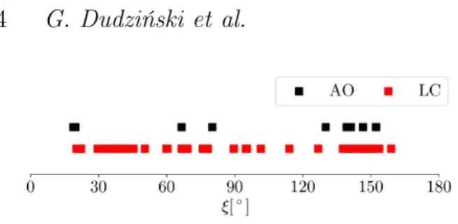
The final diameter D is calculated as follows. First, im-ages are grouped into subsets Ξjby aspect angle. In the case
of (7) Iris we established four such subsets: Ξ1 = [18◦, 20◦],
Ξ2 = [50◦, 80◦], Ξ3 = [130◦, 142◦], Ξ4 = [146◦, 152◦] (see
Fig.1). For each subset of images Ij (index j means that 1 https://imagej.net
images in a given subset have aspect angles from a set Ξj)
an weighted average Dj is computed:
Dj= P i1/δiDi P i1/δi , where ξi∈ Ξj. (3)
Then, to get diameter D, another average is computed: D = P j1/δjDj P j1/δj , (4)
where δjis an average resolution of images in a subset Ij.
When Di= Di,nom in Eq.3, we get the nominal
diam-eter value. When Di = Di,c and when we perform
calcula-tions for all of the clones, we get a set of diameters from which error bars can be extracted, i.e. the maximum Dmax and the minimum Dminvalues found in this set.
2.5 Multiresolution Photoclinometry by Deformation
Apart from SAGE and ADAM, the MPCD (Multiresolution Photoclinometry by Deformation) method was used as well to extract even more details from AO images. Additionally, this method has been modified for the purposes of this work as well to allow the calculation of errors from the fitting procedure.
The MPCD method of 3D shape reconstruction takes an initial shape model (in our case the model produced with the ADAM method) and then further modifies it to give the best fit to the AO images. The details can be found in
Capanna et al.(2013) andJorda et al.(2016). In the case of the MPCD model presented in this work, the error bars on the parameters associated to the reconstructed shape model were additionally calculated with a different method than the one described above.
The process involves two steps. First, the residuals (square of the difference between the observed and the syn-thetic pixel values, expressed in DN) are calculated for each pixel of the images used during the reconstruction. In this process, we exclude all the pixels located at the limbs and terminators on the images. These residuals are then repro-jected onto the triangular facets of the reconstructed shape model. This leads to a residual for all the facets illuminated and visible on a given image. We then compute the change of the signal in DN associated to a small variation of the direction of the normal vector of the facet. This allows us to derive the slope error of the facet (in degrees) associated to its residual value (in DN). Multiplying the slope error of the facet by the mean length of its edges leads us to a height error estimate (in km). For a given facet, these height error estimates are averaged to provide an “error map” (in km) associated to the facets of the shape model.
In the second step, we convert this local error map into uncertainties on integrated parameters such as the volume of the model. Applying a random displacement to the ver-tices of the model from the above error map would lead to physically unrealistic models with very high slopes2. As a result, we apply instead a “fractal deformation” to the re-constructed shape model. The deformation follows a fractal
2 This also is why a “smoothness” regularization term is very
often added to the objective function in clinometry methods.
ORIGINAL UNEDITED MANUSCRIPT
Figure 1. The coverage of aspect angles ξ of (7) Iris for the sets of used lightcurves (in red) and AO images (in black). Nominal pole solutions were used in calculations.
Figure 2. Resolution of AO images in km per pixel against aspect angle ξ.
law in which the sigma of the Gaussian random displace-ment distribution follows a power law with respect to the sampling of the multi-resolution models used in the MPCD method (Capanna et al. 2013). The sampling of each model is calculated as the mean edge length of all triangles. In or-der to ensure that our displacements match the error map calculated in the first step, the sigma value of the fractal law applied to the latest (highest resolution) model is set equal to the standard deviation of the map values. The fractal di-mension is taken between 2.1 and 2.3, following the analysis of NEAR/NRL laser altimetry measurements performed by NEAR for the surface of asteroid (433) Eros (Cheng et al. 2002). A large number (10000) of such “fractal random mod-els” are generated in this way. The physical parameters are calculated for each model and the calculated values repre-sent their error distribution, which is fitted by a Gaussian curve. The adopted error associated to each parameter is the fitted sigma value of the Gaussian.
3 OBSERVATIONS
This study uses 133 lightcurves in total, which were obtained at phase angles between 2.6◦ and 31.9◦ spanning 62 years (1950 – 2012) with amplitudes ranging from 0.02 to 0.35 mag. Observation characteristics are shown in Tab. A1. In addition, 57 AO images were used. 35 of which were ob-tained by the VLT/SPHERE/ZIMPOL instrument, reduced and deconvoluted with the ESO pipeline. This process is de-scribed inVernazza et al.(2018). More information on the AO images is provided in Tab.A2.
The coverage of aspect angles for all of the data is shown in Fig. 1. In Fig. 2 the resolution of AO images is shown against their aspect angles. The best quality images from
Table 1. Summary of the input data used to create the models. Note that MPCD model uses ADAM model as a starting point. The usage of individual AO images is shown in Tab.A2.
SAGE ADAM ADAM_2 MPCD
lightcurves 3 3 3 7 AO (2002) 3 3 3 7 AO (2006) 3 3 3 7 AO (2009) 3 3 3 7 AO (2010) 3 3 3 7 AO (2017) 3 3 3 3 AO (2019) 3 7 3 3
VLT/SPHERE in 2017 with 2.35 km per pixel resolution were accompanied by Keck observations with aspect angles between 130◦– 146◦, but with significantly worse resolution. Another set of VLT/SPHERE observations in 2019 at aspect 20◦covered the asteroid’s northern hemisphere, a part of the body not visible earlier. Unfortunately, due to the greater distance to the target than in 2017, the resolution of ∼ 5 km per pixel did not allow distinguishing topographical features on the surface. Also, the fact that the aspects of two of the best quality image sets are 130◦from each other looking at the target from opposite poles limits proper shape determi-nation mostly at the low latitude regions. When it comes to putting the limits on the z-scale of the (7) Iris models, the 2009 and 2010 datasets are critical as they were obtained at aspects 80◦and 67◦. Their resolution, however, is rather low (> 8 km per pixel).
4 RESULTS
4.1 Models of (7) Iris
Lightcurve and AO data of (7) Iris were used to analyse four models of this object denoted hereafter as ADAM, ADAM_2, SAGE and MPCD. The first model was cre-ated by (Hanuš et al. 2019) with the ADAM technique and did not utilise the 2019 AO images. In this work, we cre-ated three additional models (denoted as ADAM_2, SAGE and MPCD) with the ADAM, SAGE and MPCD meth-ods. The ADAM_2 and SAGE models are based on the full dataset including 2019 images. The SAGE method was developed to create lightcurve based models of asteroids (Bartczak & Dudziński 2018) and extended here to include AO images as well. The MPCD model was created with the ADAM model as a starting point which was modified to give the best fit to the subset of AO images from 2017 and 2019. (see Tab. 1 and Tab. A2 for the exact epochs). The rota-tional periods of the models are almost identical, and the pole solutions differ only by a few degrees. These values are shown in Tab.2.
The ADAM and MPCD models were created with the goal to reproduce surface details. In the first case, the model was created in two steps. In the first one, lightcurves and AO data had the same weights giving preliminary model. Then, the weights of the data were lowered with the exception of VLT/SPHERE images. In result, the topographical features were reproduced at the cost of the fit to the lightcurves. This model was fed to the MPCD method, which used 2017 and 2019 AO images alone to reproduce topographical features, and their reliability, in even more detail. The ADAM_2
ORIGINAL UNEDITED MANUSCRIPT
and SAGE models focused on explaining lightcurves and AO images simultaneously, meaning that the weights for lightcurves and AO data were not altered. Therefore, the first two models have worse fits to the lightcurves (0.0301 mag for ADAM and 0.0304 mag for MPCD) compared to the latter two (0.0254 mag for ADAM_2 and 0.0252 mag for SAGE), but they reproduce topographical features much better. The lightcurve comparison is featured in Fig. B1, while the comparison of AO images and the models’ projec-tions is featured in Fig.B2andB3.
4.2 Uncertainty assessment
All four models were subjected to uncertainty assessment using the complete dataset of lightcurves and AO images. It should be mentioned that the 2019 VLT/SPHERE observa-tions were not used to create the ADAM model of (7) Iris, and the MPCD model used the ADAM model as a starting point and used a subset of 2017 and 2019 images only. The population of accepted clones is the basis of the uncertainty of all physical parameters reported in this section.
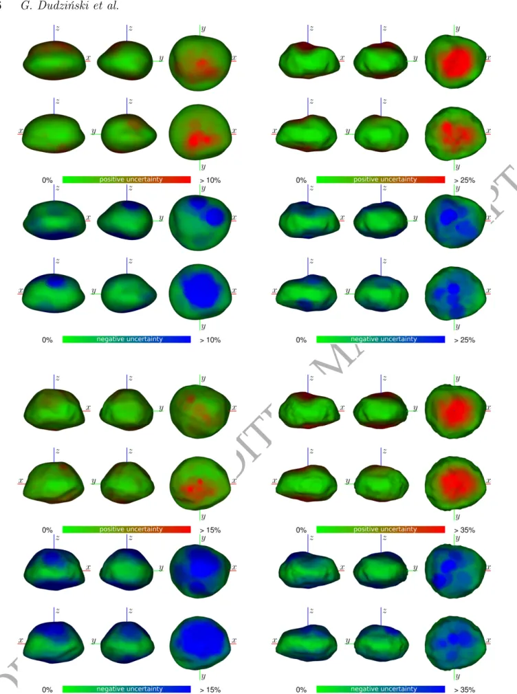
The projections of the models with the uncertainty of the shape color-coded on the surface are presented in Fig.3. The colors correspond to the level of deviation of a given vertex from the nominal position in the clone population.
To incorporate the models’ uncertainties in the size de-termination, the dimensionless clones were fitted to the AO images. From those fits, a range of values was extracted and compared with the sizes of nominal models. The di-ameters from different images were weighted as described in Sec. 2.4. The resulting equivalent sphere diameters for the models are DSAGEeq = 199+10−8 km, DADAMeq = 199+12−9 km,
DADAM_2eq = 200+10−18km and DMPCDeq = 198 +19
−17km. The fits
to individual images are shown in Fig.4, while uncertainties of the diameter, volume, rotational period and pole solution are given in Tab.2.
4.3 Uncertainty reported by MPCD method The uncertainty values for MPCD model were also obtained independently based on AO images alone and using the method described in Sec. 2.5. The resulting values and un-certainties diverge from the one reported in the previous section because both the method and dataset used were dif-ferent.
The northern and southern hemispheres of (7) Iris were observed at different resolutions during two distinct appari-tions in 2017 and 2019. We thus applied the process sep-arately for the two resolutions and added the resulting un-certainties quadratically. Finally, we doubled the uncertainty along the rotation axis because no images with an equatorial view were used.
The uncertainties on the spin-vector coordinates corre-spond to an offset of ∼1px at the limbs. The associated χ2 (square of the difference between the observed and synthetic images, in units of the instrumental noise) are also within 30% from the χ2 of the best-fit solution.
The resulting model parameters with uncertainties are: Deq = 204 ± 10 km, λ = 19 ± 3◦, β = 26 ± 3◦.
4.4 Density
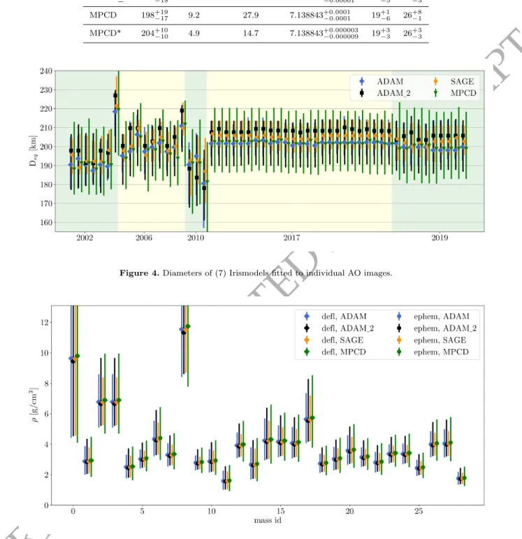
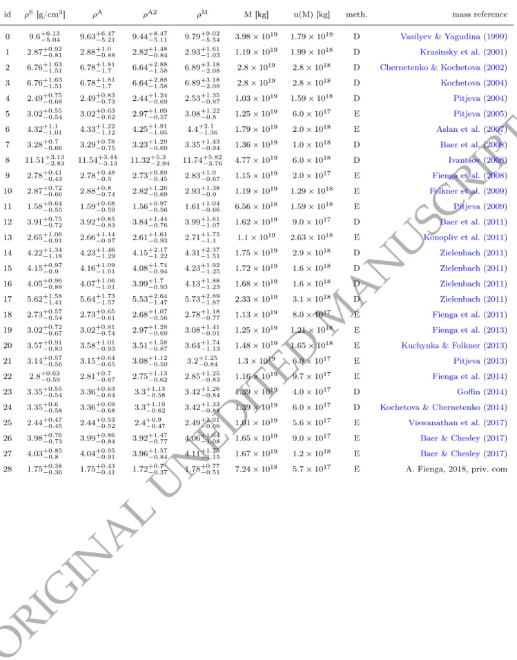
Finally, the models’ volumes were combined with the mass estimates available in the literature to calculate densities. The values are shown in Tab.C1and plotted in Fig.5. The density uncertainties come both from mass estimates’ and model uncertainties. The values vary significantly: from 1.52 to 11.51 g/cm3, averaging at 4 g/cm3 (or 3.28 g/cm3 when
4 outliers above 6 g/cm3 are disregarded). Figure 6shows the ratios of mass to volume uncertainties as contributing factors to the overall density uncertainty. The ratio for a given density puts it into one of two categories, i.e. mass and volume dominant, when the ratio is above or below 1, respectively.
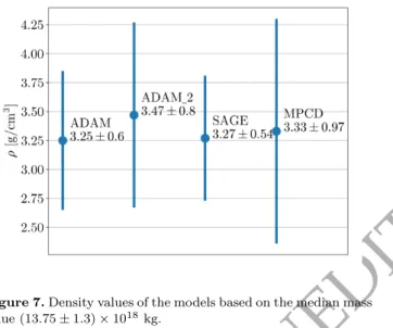
To give per model density of (7) Iris we used the proce-dure described inHanuš et al.(2019), i.e. we took the me-dian mass value from the values reported in the literature after excluding five estimates with the highest uncertainties. The value with 1σ confidence level is (13.75 ± 1.3) × 1018kg. The mass and diameter uncertainties were added in quadra-ture, yielding ρSAGE = 3.27 ± 0.54, ρADAM = 3.25 ± 0.61, ρADAM_2 = 3.47 ± 0.80 and ρMPCD = 3.33 ± 0.97 g/cm3.
The values are shown in Fig.7. 5 CONCLUSIONS
We have developed the method to assess the uncertainties of an asteroid shape modeled from lightcurves and AO im-ages. The method was used to test three models of (7) Iris produced independently by the SAGE, ADAM and MPCD modeling techniques. As a result, we calculated the uncer-tainties of physical parameters of the models (volume, rota-tional period, pole coordinates). The population of accepted clones was then used to scale the models by comparing the clones’ projections with AO images and infer the diameter of (7) Iris taking into account models’ uncertainties. The values were then used to calculate the densities.
When establishing the size of the models, the fits were weighted based on observations’ aspect angles and image resolutions to balance the information content in the data. We found the equivalent sphere diameters to be DSAGEeq =
199+10−8 km, DADAMeq = 199 +12 −9 km, D ADAM_2 eq = 200+10−18 km and DMPCD eq = 198 +19
−17km. The relative diameter
uncertain-ties of these models are 4.5%, 5.5%, 6.8% and 9.2%, respec-tively, which translate into 13.7%, 16.6%, 19.7% and 27.9% relative uncertainties in the volume. An independent un-certainty assessment with MPCD method based on a sub-set of AO images alone yielded Deq = 204 ± 10 km. The
size of (7) Iris established in this work lies within the error bars of the one presented inHanuš et al.(2019), i.e. 214 ± 5 km. However, the relative uncertainty is more than 4 times greater.
A closer look at the models’ projections (Fig. 3) in-dicates that the equatorial regions are well determined while the biggest source of uncertainty comes from the pole regions. This is consistent with the fact that relative lightcurves in practice carry close to zero information about the z-scale. Hence, the resulting z-scale was for the most part dependent on AO images with aspect angles near 90◦; since the resolution of those was poor, there was a significant amount of free play for models’ parameters at high latitudes.
ORIGINAL UNEDITED MANUSCRIPT
Figure 3. Projections of (7) Iris SAGE (top left), ADAM (top right), ADAM_2 (bottom left) and MPCD (bottom right) models. Colors represent positive (red) and negative (blue) local surface uncertainties expressed as percentage of the length of the longest vector in the model. These values come from the discrepancy of vertex positions in the population of accepted clones. Note different ranges of values for each model.
ORIGINAL UNEDITED MANUSCRIPT
Table 2. Uncertainty values of models’ parameters in reference to the nominal model; Deq – equivalent sphere diameter, u(Deq) –
relative diameter uncertainty, u(V ) – relative volume uncertainty, P – rotational period, λ and β – coordinates of the spin axis. The relative uncertainties were calculated according to the formula: urel(x) = 12(δx+− δ−x)/x · 100%, where δ+x and δx−are the upper and
lower uncertainties of x. The MPCD* corresponds to the values produced independently using the MPCD method (see Sec.2.5). method Deq [km] u(Deq) [%] u(V ) [%] P λ [◦] β [◦]
SAGE 199+10−8 4.5 13.7 7.138843+0.000003−0.000009 21+1−1 23+1−2 ADAM 199+12−9 5.5 16.6 7.138843+0.0001−0.0001 19+1−2 26+3−3 ADAM_2 200+10−18 6.8 19.7 7.138844+0.000004−0.00001 20+1−5 23+3−3 MPCD 198+19−17 9.2 27.9 7.138843+0.0001−0.0001 19+1−6 26+8−1 MPCD* 204+10−10 4.9 14.7 7.138843 +0.000003 −0.000009 19 +3 −3 26 +3 −3
Figure 4. Diameters of (7) Irismodels fitted to individual AO images.
Figure 5. Densities of (7) Iris models. Masses obtained via deflection method are marked by diamond shapes, while circles mark the ones obtained with the ephemeris method. Density and mass values with references can be found in Tab.C1.
ORIGINAL UNEDITED MANUSCRIPT
Figure 6. The ratios of mass to volume uncertainties u(ρ, M )/u(ρ, V ) as contributing factors to the overall density un-certainty. The values above or below 1 indicate that the density uncertainty is dominated by mass or volume uncertainty, respec-tively.
Figure 7. Density values of the models based on the median mass value (13.75 ± 1.3) × 1018kg.
It is also not surprising that the northern hemisphere mod-eled in the SAGE model has smaller uncertainty than in the ADAM model since the data from 2019 covering the north-ern hemisphere were not used in modelling of the latter. The ADAM_2 model is taller in z-axis from the others but has larger negative uncertainty values. This reflects the fact that the weight put on AO data compared to lightcurves in this example was smaller than in the ADAM model.
The differences between the level of detail on the sur-faces of the models are due to the different weights put on the data during the modelling. The ADAM model favored VLT/SPHERE images sacrificing the goodness of the fit of the lightcurves. This indicates some inconsistency among the two data types, which could be a result of several factors, e.g. albedo variations on the surface of (7) Iris or particu-lar scattering law used during the modelling, both influenc-ing the lightcurves and AO images in different ways. The lightcurves and AO images also covered different epochs, hence different aspect and phase angles. The reliability of the
topographical features should be therefore interpreted with this in mind. However, the results of the MPCD method, that used AO images alone with success, indicate that the topographical features are at least consistent among AO images themselves. The presence of topographical features does not influence the volume of the body in significant way, though, and do not alter our results on volume and density uncertainties.
The densities were calculated based on the mass esti-mates available in the literature (Tab.C1). The results are rather humbling in regards to what is possible to be known about the internal structure and composition of (7) Iris. Firstly, the mass estimates are not consistent with each other, hence, the computed densities vary greatly between 1.56 and 11.74 g/cm3. However, the great variability in mass estimates indicates that the error bars for the masses are vastly underestimated, thus clouding our judgement. Sec-ondly, despite the use of a big number of lightcurves and excellent quality AO images, the uncertainty method used in this work revealed that the models themselves are a source of considerable ambiguity as well. The majority of densities’ uncertainties are still volume dominant, as shown in Fig.6. If we consider the median mass after discarding five mass values with the greatest error bars and calculating 1σ confidence level, i.e. (13.75 ± 1.3) × 1018kg, we get ρSAGE= 3.27 ± 0.54, ρADAM = 3.25 ± 0.61, ρADAM_2= 3.47 ± 0.80 and ρMPCD= 3.33 ± 0.97 g/cm3
density values. The use of the median mass is dictated by the use of different methods and datasets when producing the masses. Also, because of that, the confidence level of the median comes from the dis-persion of the mass values rather than the combination of uncertainties reported in the literature.
The SAGE model has the smallest uncertainty of the four models. The uncertainty was calculated with the use of all of the available lightcurves and AO images, and the SAGE model was produced with the same dataset. More-over, the surface details were not reproduced the aim of this model being to explain all of the data as well as possi-ble simultaneously and focusing on the volume. Because the craters and other topographic features have minimal impact on the volume, the opposite happened for the MPCD model. This model reproduces the surface features with great de-tail, while not being considerate of the lightcurves as much. Each data type has its pitfalls and careful uncertainty as-sessment is essential in evaluating the results. The analysis can also be very useful in planning the future observations, e.g. to aim at the epochs that will potentially contribute new information on the target.
ACKNOWLEDGEMENTS
Based on observations collected at the European Organ-isation for Astronomical Research in the Southern Hemi-sphere under ESO programme 199.C-0074 (principal inves-tigator: P. Vernazza). This work has been supported by the Czech Science Foundation through grant 20-08218S (J.H., M.B) and by the Charles University Research program No. UNCE/SCI/023. This work has been partially supported by Horizon 2020 grant no. 871149 "EPN-2024-RI".
ORIGINAL UNEDITED MANUSCRIPT
DATA AVAILABILITY
The data underlying this article will be shared on reasonable request to the corresponding author.
REFERENCES
Aslan Z., Gumerov R., Hudkova L., Ivantsov A., Khamitov I., Pinigin G., 2007, Mass Determination of Small Solar System Bodies with Ground-based Observations. p. 52
Baer J., Chesley S. R., 2017,AJ,154, 76
Baer J., Milani A., Chesley S., Matson R. D., 2008, in AAS/Division for Planetary Sciences Meeting Abstracts #40. AAS/Division for Planetary Sciences Meeting Abstracts. p. 52.09
Baer J., Chesley S. R., Matson R. D., 2011,AJ,141, 143
Bartczak P., Dudziński G., 2018,MNRAS,473, 5050
Bartczak P., Dudziński G., 2019,MNRAS,485, 2431
Capanna C., GesquiÃĺre G., Jorda L., Lamy P., Vibert D., 2013, The Visual Computer, pp 825–835
Chang Y. C., Chang C. S., 1963, Acta Astron. Sin., 11, 139 Cheng A. F., et al., 2002,Icarus,155, 51
Chernetenko Y. A., Kochetova O. M., 2002, in Warmbein B., ed., ESA Special Publication Vol. 500, Asteroids, Comets, and Meteors: ACM 2002. pp 437–440
Fienga A., Manche H., Laskar J., Gastineau M., 2008, A&A,
477, 315
Fienga A., Kuchynka P., Laskar J., Manche H., Gastineau M., 2011, in EPSC-DPS Joint Meeting 2011. p. 1879
Fienga A., Manche H., Laskar J., Gastineau M., Verma A., 2013, arXiv e-prints,p. arXiv:1301.1510
Fienga A., Manche H., Laskar J., Gastineau M., Verma A., 2014, arXiv e-prints,p. arXiv:1405.0484
Foglia S., 1992, Minor Planet Bulletin,19, 19
Folkner W. M., Williams J. G., Boggs D. H., 2009, Interplanetary Network Progress Report,42-178, 1
Gehrels T., Owings D., 1962,ApJ,135, 906
Goffin E., 2014,A&A,565, A56
Grice J., Snodgrass C., Green S. F., Carry B., 2017, in Tancredi G., Gallardo T., FernÃąndez J. A., eds, Asteroids, Comets, Meteors 2017.
Groeneveld I., Kuiper G. P., 1954,ApJ,120, 200
Hanuš J., et al., 2019,A&A,624, A121
Hoffmann M., Geyer E. H., 1993, A&AS,101, 621
Ivantsov A., 2008,Planet. Space Sci.,56, 1857
Jorda L., et al., 2016,Icarus,277, 257
Kochetova O. M., 2004,Solar System Research,38, 66
Kochetova O. M., Chernetenko Y. A., 2014,
Solar System Research,48, 295
Konopliv A. S., Asmar S. W., Folkner W. M., Karatekin Ö., Nunes D. C., Smrekar S. E., Yoder C. F., Zuber M. T., 2011,Icarus,
211, 401
Krasinsky G. A., Pitjeva E. V., Vasilyev M. V., Yagudina E. I., 2001, Estimating Masses of Asteroids, Communications of the Institute of Applied Astronomy Russian Academy of Sciences Kuchynka P., Folkner W. M., 2013,Icarus,222, 243
Lagerkvist C. I., Williams I. P., 1987, A&AS,68, 295
Pitjeva E. V., 2004, in 35th COSPAR Scientific Assembly. p. 2014 Pitjeva E. V., 2005,Solar System Research,39, 176
Pitjeva E. V., 2009,Proceedings of the International Astronomical Union, 5, 170âĂŞ178
Pitjeva E. V., 2013,Solar System Research,47, 386
Ridler T. W., S. C., 1978, IEEE Trans. System, Man and Cyber-netics, 8, 630
Schmid H. M., et al., 2017,A&A,602, A53
Taylor R. C., 1977,AJ,82, 441
Vasilyev M., Yagudina E., 1999, Transactions of the Institute of Applied Astronomy Russian Academy of Sciences,4, 98
Vernazza P., et al., 2014,ApJ,791, 120
Vernazza P., et al., 2018, A&A, accepted
Viikinkoski M., Kaasalainen M., Durech J., 2015, A&A, 576, A8 Viikinkoski M., Hanuš J., Kaasalainen M., Marchis F., Ďurech J.,
2017,A&A,607, A117
Viswanathan V., Fienga A., Gastineau M., Laskar J., 2017,
Notes Scientifiques et Techniques de l’Institut de Mecanique Celeste,
108
Zhou X. H., Yang X. Y., Wu Z. X., 1982, Acta Astronomica Sinica,
23, 349
Zielenbach W., 2011,AJ,142, 120
van Houten-Groeneveld I., van Houten C. J., 1958,ApJ,127, 253
ORIGINAL UNEDITED MANUSCRIPT
APPENDIX A: OBSERVATIONS
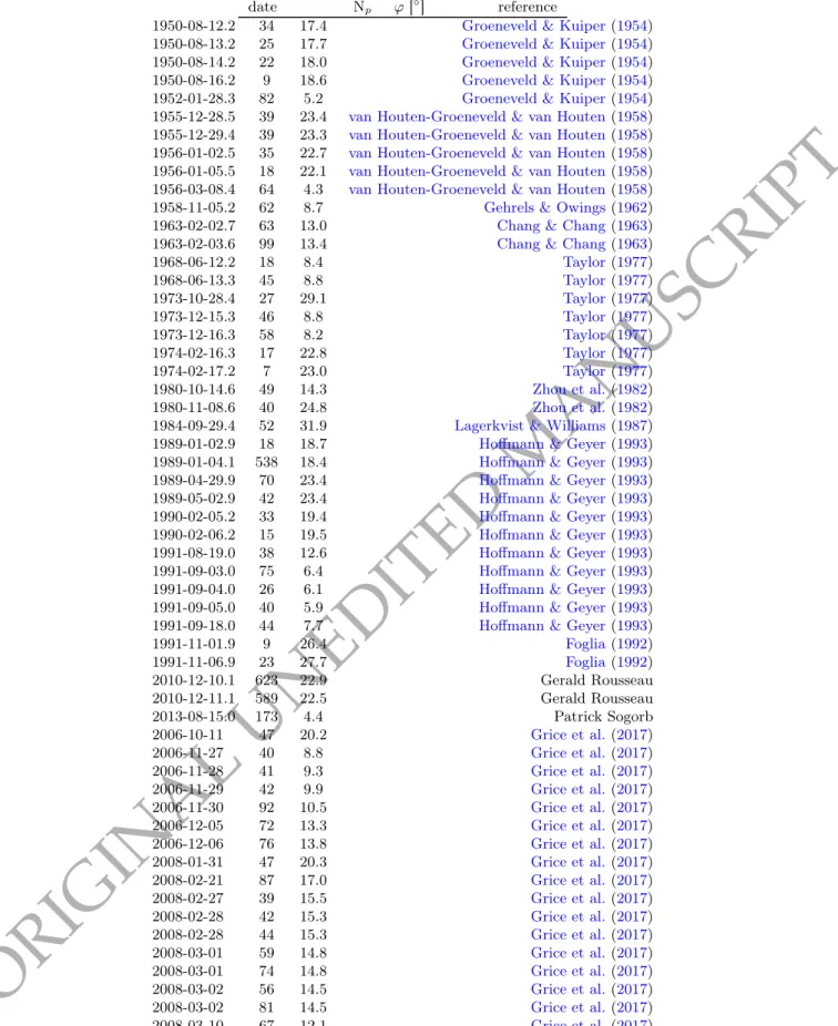
Table A1: Details of the lightcurves used in the modelling process. Npdenotes the number of photometric points in a lightcurve,
ϕ denotes the phase angle.
date Np ϕ [◦] reference
1950-08-12.2 34 17.4 Groeneveld & Kuiper(1954) 1950-08-13.2 25 17.7 Groeneveld & Kuiper(1954) 1950-08-14.2 22 18.0 Groeneveld & Kuiper(1954) 1950-08-16.2 9 18.6 Groeneveld & Kuiper(1954) 1952-01-28.3 82 5.2 Groeneveld & Kuiper(1954) 1955-12-28.5 39 23.4 van Houten-Groeneveld & van Houten(1958) 1955-12-29.4 39 23.3 van Houten-Groeneveld & van Houten(1958) 1956-01-02.5 35 22.7 van Houten-Groeneveld & van Houten(1958) 1956-01-05.5 18 22.1 van Houten-Groeneveld & van Houten(1958) 1956-03-08.4 64 4.3 van Houten-Groeneveld & van Houten(1958) 1958-11-05.2 62 8.7 Gehrels & Owings(1962) 1963-02-02.7 63 13.0 Chang & Chang(1963) 1963-02-03.6 99 13.4 Chang & Chang(1963) 1968-06-12.2 18 8.4 Taylor(1977) 1968-06-13.3 45 8.8 Taylor(1977) 1973-10-28.4 27 29.1 Taylor(1977) 1973-12-15.3 46 8.8 Taylor(1977) 1973-12-16.3 58 8.2 Taylor(1977) 1974-02-16.3 17 22.8 Taylor(1977) 1974-02-17.2 7 23.0 Taylor(1977) 1980-10-14.6 49 14.3 Zhou et al.(1982) 1980-11-08.6 40 24.8 Zhou et al.(1982) 1984-09-29.4 52 31.9 Lagerkvist & Williams(1987) 1989-01-02.9 18 18.7 Hoffmann & Geyer(1993) 1989-01-04.1 538 18.4 Hoffmann & Geyer(1993) 1989-04-29.9 70 23.4 Hoffmann & Geyer(1993) 1989-05-02.9 42 23.4 Hoffmann & Geyer(1993) 1990-02-05.2 33 19.4 Hoffmann & Geyer(1993) 1990-02-06.2 15 19.5 Hoffmann & Geyer(1993) 1991-08-19.0 38 12.6 Hoffmann & Geyer(1993) 1991-09-03.0 75 6.4 Hoffmann & Geyer(1993) 1991-09-04.0 26 6.1 Hoffmann & Geyer(1993) 1991-09-05.0 40 5.9 Hoffmann & Geyer(1993) 1991-09-18.0 44 7.7 Hoffmann & Geyer(1993) 1991-11-01.9 9 26.4 Foglia(1992) 1991-11-06.9 23 27.7 Foglia(1992) 2010-12-10.1 623 22.9 Gerald Rousseau 2010-12-11.1 589 22.5 Gerald Rousseau 2013-08-15.0 173 4.4 Patrick Sogorb 2006-10-11 47 20.2 Grice et al.(2017) 2006-11-27 40 8.8 Grice et al.(2017) 2006-11-28 41 9.3 Grice et al.(2017) 2006-11-29 42 9.9 Grice et al.(2017) 2006-11-30 92 10.5 Grice et al.(2017) 2006-12-05 72 13.3 Grice et al.(2017) 2006-12-06 76 13.8 Grice et al.(2017) 2008-01-31 47 20.3 Grice et al.(2017) 2008-02-21 87 17.0 Grice et al.(2017) 2008-02-27 39 15.5 Grice et al.(2017) 2008-02-28 42 15.3 Grice et al.(2017) 2008-02-28 44 15.3 Grice et al.(2017) 2008-03-01 59 14.8 Grice et al.(2017) 2008-03-01 74 14.8 Grice et al.(2017) 2008-03-02 56 14.5 Grice et al.(2017) 2008-03-02 81 14.5 Grice et al.(2017) 2008-03-10 67 12.1 Grice et al.(2017)
ORIGINAL UNEDITED MANUSCRIPT
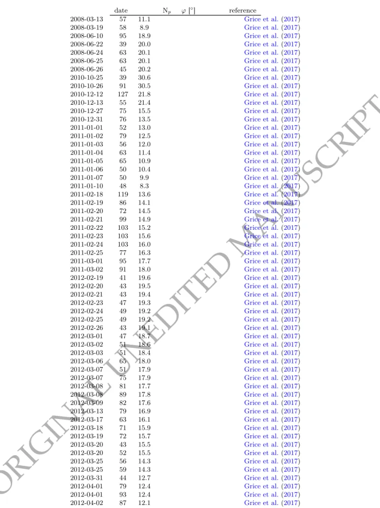
Table A1: continued
date Np ϕ [◦] reference 2008-03-13 57 11.1 Grice et al.(2017) 2008-03-19 58 8.9 Grice et al.(2017) 2008-06-10 95 18.9 Grice et al.(2017) 2008-06-22 39 20.0 Grice et al.(2017) 2008-06-24 63 20.1 Grice et al.(2017) 2008-06-25 63 20.1 Grice et al.(2017) 2008-06-26 45 20.2 Grice et al.(2017) 2010-10-25 39 30.6 Grice et al.(2017) 2010-10-26 91 30.5 Grice et al.(2017) 2010-12-12 127 21.8 Grice et al.(2017) 2010-12-13 55 21.4 Grice et al.(2017) 2010-12-27 75 15.5 Grice et al.(2017) 2010-12-31 76 13.5 Grice et al.(2017) 2011-01-01 52 13.0 Grice et al.(2017) 2011-01-02 79 12.5 Grice et al.(2017) 2011-01-03 56 12.0 Grice et al.(2017) 2011-01-04 63 11.4 Grice et al.(2017) 2011-01-05 65 10.9 Grice et al.(2017) 2011-01-06 50 10.4 Grice et al.(2017) 2011-01-07 50 9.9 Grice et al.(2017) 2011-01-10 48 8.3 Grice et al.(2017) 2011-02-18 119 13.6 Grice et al.(2017) 2011-02-19 86 14.1 Grice et al.(2017) 2011-02-20 72 14.5 Grice et al.(2017) 2011-02-21 99 14.9 Grice et al.(2017) 2011-02-22 103 15.2 Grice et al.(2017) 2011-02-23 103 15.6 Grice et al.(2017) 2011-02-24 103 16.0 Grice et al.(2017) 2011-02-25 77 16.3 Grice et al.(2017) 2011-03-01 95 17.7 Grice et al.(2017) 2011-03-02 91 18.0 Grice et al.(2017) 2012-02-19 41 19.6 Grice et al.(2017) 2012-02-20 43 19.5 Grice et al.(2017) 2012-02-21 43 19.4 Grice et al.(2017) 2012-02-23 47 19.3 Grice et al.(2017) 2012-02-24 49 19.2 Grice et al.(2017) 2012-02-25 49 19.2 Grice et al.(2017) 2012-02-26 43 19.1 Grice et al.(2017) 2012-03-01 47 18.7 Grice et al.(2017) 2012-03-02 51 18.6 Grice et al.(2017) 2012-03-03 51 18.4 Grice et al.(2017) 2012-03-06 65 18.0 Grice et al.(2017) 2012-03-07 51 17.9 Grice et al.(2017) 2012-03-07 75 17.9 Grice et al.(2017) 2012-03-08 81 17.7 Grice et al.(2017) 2012-03-08 89 17.8 Grice et al.(2017) 2012-03-09 82 17.6 Grice et al.(2017) 2012-03-13 79 16.9 Grice et al.(2017) 2012-03-17 63 16.1 Grice et al.(2017) 2012-03-18 71 15.9 Grice et al.(2017) 2012-03-19 72 15.7 Grice et al.(2017) 2012-03-20 43 15.5 Grice et al.(2017) 2012-03-20 52 15.5 Grice et al.(2017) 2012-03-25 56 14.3 Grice et al.(2017) 2012-03-25 59 14.3 Grice et al.(2017) 2012-03-31 44 12.7 Grice et al.(2017) 2012-04-01 79 12.4 Grice et al.(2017) 2012-04-01 93 12.4 Grice et al.(2017) 2012-04-02 87 12.1 Grice et al.(2017)
ORIGINAL UNEDITED MANUSCRIPT
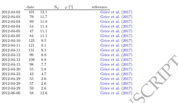
Table A1: continued
date Np ϕ [◦] reference 2012-04-02 101 12.1 Grice et al.(2017) 2012-04-03 79 11.7 Grice et al.(2017) 2012-04-03 89 11.8 Grice et al.(2017) 2012-04-04 54 11.4 Grice et al.(2017) 2012-04-05 47 11.1 Grice et al.(2017) 2012-04-05 84 11.1 Grice et al.(2017) 2012-04-10 125 9.5 Grice et al.(2017) 2012-04-11 121 9.1 Grice et al.(2017) 2012-04-11 131 9.1 Grice et al.(2017) 2012-04-12 99 8.8 Grice et al.(2017) 2012-04-12 109 8.8 Grice et al.(2017) 2012-04-15 98 7.7 Grice et al.(2017) 2012-04-20 55 5.8 Grice et al.(2017) 2012-04-23 43 4.7 Grice et al.(2017) 2012-04-29 55 2.6 Grice et al.(2017) 2012-04-29 57 2.6 Grice et al.(2017) 2012-04-29 59 2.6 Grice et al.(2017) 2012-06-06 58 12.6 Grice et al.(2017)
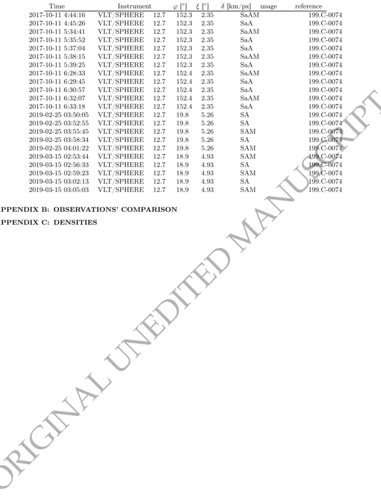
Table A2: Details of Adaptive Optics observations used in the modelling process. ϕ – phase angle, ξ – aspect angle, δ – resolution. A letter corresponding to a model appears in the "usage" column if an image has been used during the modelling: S – SAGE, a – ADAM, A – ADAM_2, M – MPCD.
Time Instrument ϕ [◦] ξ [◦] δ [km/px] usage reference 2002-08-05 14:42:06 Keck/NIRC2 12.3 139.3 8.69 SaA N10N2 2002-08-05 14:45:29 Keck/NIRC2 12.3 139.3 8.69 SaA N10N2 2002-08-05 14:48:25 Keck/NIRC2 12.3 139.3 8.69 SaA N10N2 2002-08-05 15:11:44 Keck/NIRC2 12.3 139.3 8.69 SaA N10N2 2002-08-05 15:14:34 Keck/NIRC2 12.3 139.3 8.69 SaA N10N2 2002-09-27 09:54:15 Keck/NIRC2 17.5 130.1 8.23 SaA Viikinkoski et al.(2017) 2002-12-29 04:35:18 Keck/NIRC2 30.4 146.6 13.59 SaA Viikinkoski et al.(2017) 2006-11-17 07:06:23 Keck/NIRC2 3.3 141.2 6.14 SaA Viikinkoski et al.(2017) 2006-11-17 07:13:20 Keck/NIRC2 3.3 141.2 6.14 SaA Viikinkoski et al.(2017) 2006-11-17 07:18:58 Keck/NIRC2 3.3 141.2 6.14 SaA Viikinkoski et al.(2017) 2006-11-17 07:53:59 Keck/NIRC2 3.3 141.2 6.14 SaA Viikinkoski et al.(2017) 2006-11-17 07:57:52 Keck/NIRC2 3.3 141.2 6.14 SaA Viikinkoski et al.(2017) 2006-11-17 08:02:23 Keck/NIRC2 3.3 141.3 6.14 SaA Viikinkoski et al.(2017) 2006-11-17 08:24:30 Keck/NIRC2 3.3 141.3 6.14 SaA Viikinkoski et al.(2017) 2006-11-17 08:27:22 Keck/NIRC2 3.3 141.3 6.14 SaA Viikinkoski et al.(2017) 2006-11-17 08:30:57 Keck/NIRC2 3.3 141.3 6.14 SaA Viikinkoski et al.(2017) 2009-08-16 07:50:06 Keck/NIRC2 18.1 80.1 8.2 SaA Viikinkoski et al.(2017) 2009-08-16 08:15:57 Keck/NIRC2 18.1 80.1 8.2 SaA Viikinkoski et al.(2017) 2010-12-13 06:05:38 VLT/NaCo 21.7 66.6 12.41 SaA 086.C-0785 2010-12-13 06:55:02 VLT/NaCo 21.7 66.6 12.41 SaA 086.C-0785 2010-12-14 05:24:30 VLT/NaCo 21.4 66.6 12.35 SaA 086.C-0785 2017-10-10 3:56:12 VLT/SPHERE 13.2 152.2 2.36 SaAM 199.C-0074 2017-10-10 3:57:22 VLT/SPHERE 13.2 152.2 2.36 SaA 199.C-0074 2017-10-10 3:58:33 VLT/SPHERE 13.2 152.2 2.36 SaA 199.C-0074 2017-10-10 3:59:43 VLT/SPHERE 13.2 152.2 2.36 SaA 199.C-0074 2017-10-10 4:00:55 VLT/SPHERE 13.2 152.2 2.36 SaAM 199.C-0074 2017-10-10 4:07:50 VLT/SPHERE 13.2 152.2 2.36 SaAM 199.C-0074 2017-10-10 4:09:01 VLT/SPHERE 13.2 152.2 2.36 SaA 199.C-0074 2017-10-10 4:10:12 VLT/SPHERE 13.2 152.2 2.36 SaA 199.C-0074 2017-10-10 4:11:22 VLT/SPHERE 13.2 152.2 2.36 SaA 199.C-0074 2017-10-10 4:12:32 VLT/SPHERE 13.2 152.2 2.36 SaA 199.C-0074 2017-10-11 4:40:41 VLT/SPHERE 12.7 152.3 2.35 SaAM 199.C-0074 2017-10-11 4:41:53 VLT/SPHERE 12.7 152.3 2.35 SaA 199.C-0074 2017-10-11 4:43:05 VLT/SPHERE 12.7 152.3 2.35 SaA 199.C-0074
ORIGINAL UNEDITED MANUSCRIPT
Table A2: continued
Time Instrument ϕ [◦] ξ [◦] δ [km/px] usage reference 2017-10-11 4:44:16 VLT/SPHERE 12.7 152.3 2.35 SaAM 199.C-0074 2017-10-11 4:45:26 VLT/SPHERE 12.7 152.3 2.35 SaA 199.C-0074 2017-10-11 5:34:41 VLT/SPHERE 12.7 152.3 2.35 SaAM 199.C-0074 2017-10-11 5:35:52 VLT/SPHERE 12.7 152.3 2.35 SaA 199.C-0074 2017-10-11 5:37:04 VLT/SPHERE 12.7 152.3 2.35 SaA 199.C-0074 2017-10-11 5:38:15 VLT/SPHERE 12.7 152.3 2.35 SaAM 199.C-0074 2017-10-11 5:39:25 VLT/SPHERE 12.7 152.3 2.35 SaA 199.C-0074 2017-10-11 6:28:33 VLT/SPHERE 12.7 152.4 2.35 SaAM 199.C-0074 2017-10-11 6:29:45 VLT/SPHERE 12.7 152.4 2.35 SaA 199.C-0074 2017-10-11 6:30:57 VLT/SPHERE 12.7 152.4 2.35 SaA 199.C-0074 2017-10-11 6:32:07 VLT/SPHERE 12.7 152.4 2.35 SaAM 199.C-0074 2017-10-11 6:33:18 VLT/SPHERE 12.7 152.4 2.35 SaA 199.C-0074 2019-02-25 03:50:05 VLT/SPHERE 12.7 19.8 5.26 SA 199.C-0074 2019-02-25 03:52:55 VLT/SPHERE 12.7 19.8 5.26 SA 199.C-0074 2019-02-25 03:55:45 VLT/SPHERE 12.7 19.8 5.26 SAM 199.C-0074 2019-02-25 03:58:34 VLT/SPHERE 12.7 19.8 5.26 SA 199.C-0074 2019-02-25 04:01:22 VLT/SPHERE 12.7 19.8 5.26 SAM 199.C-0074 2019-03-15 02:53:44 VLT/SPHERE 12.7 18.9 4.93 SAM 199.C-0074 2019-03-15 02:56:33 VLT/SPHERE 12.7 18.9 4.93 SA 199.C-0074 2019-03-15 02:59:23 VLT/SPHERE 12.7 18.9 4.93 SAM 199.C-0074 2019-03-15 03:02:13 VLT/SPHERE 12.7 18.9 4.93 SA 199.C-0074 2019-03-15 03:05:03 VLT/SPHERE 12.7 18.9 4.93 SAM 199.C-0074 APPENDIX B: OBSERVATIONS’ COMPARISON
APPENDIX C: DENSITIES
ORIGINAL UNEDITED MANUSCRIPT
Figure B1. Comparison of synthetic models’ lightcurves with selected observations of (7) Iris.ORIGINAL UNEDITED MANUSCRIPT
Figure B2. Comparison of the models’ projections with some of the AO images used in the study.ORIGINAL UNEDITED MANUSCRIPT
Figure B3. Comparison of the models’ projections with some of the AO images used in the study.ORIGINAL UNEDITED MANUSCRIPT
Table C1. Compilation of density values ρ of (7) Irisbased on various mass estimates. Indexes S, A, A2 and M refer to SAGE, ADAM ADAM_2 and MPCD models, respectively. Column "meth." denotes a method used for mass calculation: D – deflection, E – ephemeris. id ρS[g/cm3] ρA ρA2 ρM M [kg] u(M) [kg] meth. mass reference
0 9.6+6.13−5.04 9.63+6.47−5.21 9.44+8.47−5.11 9.79+9.02−5.54 3.98 × 10¹⁹ 1.79 × 10¹⁹ D Vasilyev & Yagudina(1999)
1 2.87+0.92−0.81 2.88+1.0−0.88 2.82+1.48−0.84 2.93+1.61−1.03 1.19 × 10¹⁹ 1.99 × 10¹⁸ D Krasinsky et al.(2001)
2 6.76+1.63−1.51 6.78+1.81−1.7 6.64+2.88−1.58 6.89+3.18−2.08 2.8 × 10¹⁹ 2.8 × 10¹⁸ D Chernetenko & Kochetova(2002)
3 6.76+1.63−1.51 6.78 +1.81 −1.7 6.64 +2.88 −1.58 6.89 +3.18 −2.08 2.8 × 10¹⁹ 2.8 × 10¹⁸ D Kochetova(2004) 4 2.49+0.75−0.68 2.49+0.83−0.73 2.44+1.24−0.69 2.53+1.35−0.87 1.03 × 10¹⁹ 1.59 × 10¹⁸ D Pitjeva(2004) 5 3.02+0.55−0.54 3.02 +0.63 −0.62 2.97 +1.09 −0.57 3.08 +1.22 −0.8 1.25 × 10¹⁹ 6.0 × 10¹⁷ E Pitjeva(2005) 6 4.32+1.1−1.01 4.33+1.22−1.12 4.25+1.91−1.05 4.4+2.1−1.36 1.79 × 10¹⁹ 2.0 × 10¹⁸ E Aslan et al.(2007) 7 3.28+0.7−0.66 3.29+0.78−0.75 3.23+1.29−0.69 3.35+1.43−0.94 1.36 × 10¹⁹ 1.0 × 10¹⁸ D Baer et al.(2008) 8 11.51+3.13−2.83 11.54+3.44−3.13 11.32+5.3−2.94 11.74+5.82−3.76 4.77 × 10¹⁹ 6.0 × 10¹⁸ D Ivantsov(2008) 9 2.78+0.41−0.43 2.78+0.48−0.5 2.73+0.89−0.45 2.83+1.0−0.67 1.15 × 10¹⁹ 2.0 × 10¹⁷ E Fienga et al.(2008) 10 2.87+0.72−0.66 2.88 +0.8 −0.74 2.82 +1.26 −0.69 2.93 +1.38 −0.9 1.19 × 10¹⁹ 1.29 × 10¹⁸ E Folkner et al.(2009) 11 1.58+0.64−0.55 1.59+0.68−0.59 1.56+0.97−0.56 1.61+1.04−0.66 6.56 × 10¹⁸ 1.59 × 10¹⁸ E Pitjeva(2009) 12 3.91+0.75−0.72 3.92+0.85−0.83 3.84+1.44−0.76 3.99+1.61−1.07 1.62 × 10¹⁹ 9.0 × 10¹⁷ D Baer et al.(2011) 13 2.65+1.06−0.91 2.66+1.14−0.97 2.61+1.61−0.93 2.71+1.75−1.1 1.1 × 10¹⁹ 2.63 × 10¹⁸ E Konopliv et al.(2011) 14 4.22+1.34−1.18 4.23+1.46−1.29 4.15+2.17−1.22 4.31+2.37−1.51 1.75 × 10¹⁹ 2.9 × 10¹⁸ D Zielenbach(2011) 15 4.15+0.97−0.9 4.16 +1.09 −1.01 4.08 +1.74 −0.94 4.23 +1.92 −1.25 1.72 × 10¹⁹ 1.6 × 10¹⁸ D Zielenbach(2011) 16 4.05+0.96−0.88 4.07+1.06−1.01 3.99+1.7−0.93 4.13+1.88−1.23 1.68 × 10¹⁹ 1.6 × 10¹⁸ D Zielenbach(2011) 17 5.62+1.58−1.41 5.64 +1.73 −1.57 5.53 +2.64 −1.47 5.73 +2.89 −1.87 2.33 × 10¹⁹ 3.1 × 10¹⁸ D Zielenbach(2011) 18 2.73+0.57−0.54 2.73+0.65−0.61 2.68+1.07−0.56 2.78+1.18−0.77 1.13 × 10¹⁹ 8.0 × 10¹⁷ E Fienga et al.(2011) 19 3.02+0.72−0.67 3.02+0.81−0.74 2.97+1.28−0.69 3.08+1.41−0.91 1.25 × 10¹⁹ 1.21 × 10¹⁸ E Fienga et al.(2013)
20 3.57+0.91−0.83 3.58+1.01−0.93 3.51+1.58−0.87 3.64+1.74−1.13 1.48 × 10¹⁹ 1.65 × 10¹⁸ E Kuchynka & Folkner(2013)
21 3.14+0.57−0.56 3.15+0.64−0.65 3.08+1.12−0.59 3.2+1.25−0.84 1.3 × 10¹⁹ 6.0 × 10¹⁷ E Pitjeva(2013) 22 2.8+0.63−0.59 2.81 +0.7 −0.67 2.75 +1.13 −0.62 2.85 +1.25 −0.83 1.16 × 10¹⁹ 9.7 × 10¹⁷ E Fienga et al.(2014) 23 3.35+0.55−0.54 3.36+0.63−0.64 3.3+1.13−0.58 3.42+1.26−0.84 1.39 × 10¹⁹ 4.0 × 10¹⁷ D Goffin(2014)
24 3.35+0.6−0.58 3.36+0.69−0.68 3.3+1.19−0.62 3.42+1.33−0.88 1.39 × 10¹⁹ 6.0 × 10¹⁷ D Kochetova & Chernetenko(2014)
25 2.44+0.47−0.45 2.44+0.53−0.52 2.4+0.9−0.47 2.49+1.01−0.66 1.01 × 10¹⁹ 5.6 × 10¹⁷ E Viswanathan et al.(2017)
26 3.98+0.76−0.73 3.99+0.86−0.84 3.92+1.47−0.77 4.06+1.64−1.08 1.65 × 10¹⁹ 9.0 × 10¹⁷ E Baer & Chesley(2017)
27 4.03+0.85−0.8 4.04 +0.95 −0.91 3.96 +1.57 −0.84 4.11 +1.75
−1.15 1.67 × 10¹⁹ 1.2 × 10¹⁸ E Baer & Chesley(2017)
28 1.75+0.38−0.36 1.75+0.43−0.41 1.72−0.37+0.7 1.78+0.77−0.51 7.24 × 10¹⁸ 5.7 × 10¹⁷ E A. Fienga, 2018, priv. com