Analytical estimate for low-altitude ENA emissivity
J. Goldstein1,2, D. V. Bisikalo3, V. I. Shematovich3, J.-C. Gérard4, F. Søraas5, D. J. McComas1,2, P. W. Valek1,2, K. LLera1,2, and J. Redfern6
1Space Science Division, Southwest Research Institute, San Antonio, Texas, USA,2Department of Physics and Astronomy,
University of Texas at San Antonio, San Antonio, Texas, USA,3Institute of Astronomy, Russian Academy of Science, Moscow,
Russia,4Institut d’Astrophysique et de Géophysique, Universite de Liège, Liège, Belgium,5Birkeland Centre for Space
Science, University of Bergen, Bergen, Norway,6Department of Space Studies, Southwest Research Institute, Boulder,
Colorado, USA
Abstract
We formulate the first analytical model for energetic neutral atom (ENA) emissivity that partially corrects for the global viewing geometry dependence of low-altitude emissions (LAEs) observed by Two Wide-angle Imaging Neutral-atom Spectrometers (TWINS). The emissivity correction requires the pitch angle distribution (PAD) and geophysical location of low-altitude ENAs. To estimate PAD, we create an energy-dependent analytical model, based on a Monte Carlo simulation. We account for energy binning by integrating model PAD over each energy bin. We account for finite angular pixels by computing emissivity as an integral over the pitch angle range sampled by the pixel. We investigate location uncertainty in TWINS pixels by performing nine variations of the emissivity calculation. Using TWINS 2 ENA imaging data from 1131 to 1145 UT on 6 April 2010, we derive emissivity-corrected ion fluxes for two angular pixel sizes: 4∘ and 1∘. To evaluate the method, we compare TWINS-derived ion fluxes to simultaneous in situ data from the National Oceanic and Atmospheric Administration (NOAA) 17 satellite. The TWINS-NOAA agreement for emissivity-corrected flux is improved by up to a factor of 7, compared to uncorrected flux. The highest 1∘ pixel fluxes are a factor of 2 higher than for 4∘ pixels, consistent with pixel-derived fluxes that are artificially low because subpixel structures are smoothed out, and indicating a possible slight advantage to oversampling the instrument-measured LAE signal. Both TWINS and NOAA ion fluxes decrease westward of 2000 magnetic local time. The TWINS-NOAA comparison indicates that the global ion precipitation oval comprises multiple smaller-scale (3–5∘ of latitude) structures.1. Introduction
The Two Wide-angle Imaging Neutral-atom Spectrometers (TWINS) mission flies two spacecraft in Molniya orbits to achieve stereo imaging of the Earth’s magnetosphere [McComas et al., 2009]. The TWINS 1 and 2 imagers measure energetic neutral atoms (ENAs) created by charge exchange in the terrestrial ring current, over the range 1–100 keV/amu, with nominal 4∘ × 4∘ angular resolution, at an ∼1 min cadence. TWINS stereo ENA observations have advanced our understanding of ring current dynamics at both high and low altitudes [Goldstein and McComas, 2013]. This paper focuses on the near-Earth ENA signal known as the low-altitude emission (LAE). The LAE is a bright feature of ENA images produced by ions in the oxygen exobase [Galand et al., 1998; Roelof and Skinner, 2000; Brandt et al., 2001a]. Observations of LAEs span two decades, via rocket-borne and satellite-based observatories [Søraas and Aarsnes, 1996; Brandt et al., 2001b; Pollock et al., 2001; Mitchell et al., 2003; Pollock et al., 2009; Bazell et al., 2010; Valek et al., 2010; Buzulukova et al., 2013; McComas et al., 2012; Søraas and Sørbø, 2013; Goldstein et al., 2013].
LAEs are a product of the interaction between mirroring or precipitating ions (both auroral and subauroral) and atomic oxygen in the 200–800 km, optically thick O exobase [Galand et al., 1998; Roelof and Skinner, 2000; Brandt et al., 2001a, 2005; Bazell et al., 2010; LLera et al., 2014] (K. LLera et al., Low-altitude emission of energetic neutral atoms: Multiple interactions and energy loss, submitted to Journal of Geophysics Research., 2015). Before escaping as ENAs, particles may undergo hundreds of charge exchange and stripping interac-tions (i.e., changing charge state from ion to neutral or vice versa), which affects their energy and pitch angle distributions (PADs). Because the PADs of these emergent ENAs are highly anisotropic, i.e., sharply peaked at large pitch angles, the ability to image LAEs is strongly dependent on viewing geometry. For a given
RESEARCH ARTICLE
10.1002/2015JA021773
Key Points:
• Analytical model of low-altitude ENA emissivity depends on local PAD and geometry
• Emissivity-corrected TWINS ion fluxes evaluated using in situ NOAA data • Global ion precipitation oval
comprises multiple smaller-scale structures Correspondence to: J. Goldstein, [email protected] Citation: Goldstein, J., D. V. Bisikalo, V. I. Shematovich, J.-C. Gérard, F. Søraas, D. J. McComas, P. W. Valek, K. LLera, and J. Redfern (2016), Analytical estimate for low-altitude ENA emissivity, J. Geophys. Res.
Space Physics, 121, 1167–1191,
doi:10.1002/2015JA021773.
Received 11 AUG 2015 Accepted 31 DEC 2015
Accepted article online 5 JAN 2016 Published online 6 FEB 2016
©2016. American Geophysical Union. All Rights Reserved.
Figure 1. TWINS LAE: example and viewing geometry. (a) Example low-altitude emission image by TWINS 2,
1131–1145 UT on 6 April 2010. Dipole field lines drawn atL = [4, 8]at four cardinal MLT values. Blue circle is the Earth’s limb. (b) TWINS 2 orbit and location at UT midpoint of interval. (c) LAE viewing geometry with definition of vectors and angles, adapted from Goldstein et al. [2013].
imager location, the apparent ENA brightness varies with source location, because each pixel’s line of sight (LOS) samples a different (and narrow) range of local pitch angle. Following Bazell et al. [2010], this viewing geometry-dependent LAE brightness function is herein denoted as the emissivity (although we use a slightly different definition; cf. section 2.3). The emissivity function quantifies the portion of an imager’s field of view for which the viewing geometry favors LAE imaging, independent of any geophysical (ion flux) variation. Bazell et al. [2010] introduced a thick target approximation (TTA) to simulate ENA propagation in the oxygen exobase and determine LAE emissivity. Their calculation assumes that ion precipitation is globally uniform (independent of latitude and local time) in order to separate viewing geometry effects from actual, i.e., geophysical, variation with magnetic local time (MLT). The emissivity function varies strongly with viewing geometry. For an imager located at magnetic local time MLTS, the theoretical emissivity is a crescent-shaped
region at or within the Earth’s limb, centered roughly 12 MLT hours away from the imager, i.e., at MLTP = MLTS+ 12. The emissivity falls off steeply with local time in either direction away from the peak at
MLTPand with increasing latitude away from the limb. Bazell et al. [2010] computed emissivity crescents for a
weakly disturbed (Dst ∼ −65 nT) event, yielding a favorable comparison between TWINS-derived ion spectra and simultaneous low-altitude (825 km) in situ data.
Figure 1a shows an example of an LAE observed by TWINS 2 on 6 April 2010 [Goldstein et al., 2013]. This example interval is used as a case study for the remainder of this paper. The LAE is the bright region of high (∼4–40 [cm2sr s keV]−1) flux near the Earth’s limb. For reference, the blue circle marks the limb at 1 Earth
radius (RE). The highest flux for r ≤ 1 REis indeed a crescent-shaped region, inside the limb opposite TWINS 2. At the time of the image, TWINS 2 was located (cf. orbit plot of Figure 1b) at geocentric radius rS = 5.6 RE, magnetic latitude ΛS= 59.3∘, and MLTS= 1035. The peak limb flux occurs approximately 12 MLT hours from TWINS 2, at MLTP≈ 2235 (cf. close-up view in Figure 1a), and high ENA flux along the limb is localized within ±3 MLT hours of the peak. Thus, consistent with the theoretical emissivity [Bazell et al., 2010], the observed LAE intensity varies strongly with viewing geometry, specifically with the relative MLT between the imager and the ENA source location. Note that in this study we assume that the LAEs are composed of hydrogen ENAs only, with no contribution from oxygen [Valek et al., 2013]. This assumption is justified for the 50 keV/amu image in Figure 1; the contribution from ∼0.8 MeV O ENAs is likely to be very small. The goal of ENA image analysis
is to obtain global quantitative information (flux, spatial distribution, and spectra) about the parent ring cur-rent ions. For low-altitude ions, it is necessary to factor out the MLT-dependent emissivity function that can obscure the actual local time dependence of the ions. Because of the computational expense of a full simula-tion of the thick target region [Bazell et al., 2010], for routine LAE analysis it is beneficial to have the choice of a less expensive means of estimating limb ENA emissivity. In this paper we circumvent the numerical calcula-tion of the emissivity funccalcula-tion by deriving a simple analytical form based on purely geometrical analysis and with the aid of an analytical model of low-altitude ENA pitch angle that is based on kinetic simulation results. The rest of this paper is organized as follows. In section 2 we introduce an analytical model of LAE emissivity that depends on viewing geometry and local pitch angle of the ENA source. This emissivity model formula-tion motivates the rest of the paper. Quantifying the emissivity requires a model for low-altitude ENA pitch angle. Therefore, in section 3 we generate an analytical pitch angle model, based on a computer simulation of the thick target region. In section 4 we apply the emissivity model (with its included pitch angle model) to the TWINS 2 50 keV image of Figure 1. Emissivity-corrected TWINS ion fluxes are compared with simultaneous in situ (NOAA) data in section 5. We find that applying the emissivity correction improves the TWINS-NOAA agreement by as much as a factor of 7 and enables a more direct comparison of single TWINS pixels to indi-vidual NOAA ion peaks. In sections 6 and 7 we discuss and summarize our results. Appendix B formulates an ad hoc empirical model of ion precipitation, and Appendix B discusses observations of low-altitude ENAs.
2. Geometrical Emissivity
In this section we introduce an analytical emissivity that depends on the imager location and the local pitch angle (PA) in the low-altitude emission region. The geometrical relations are adopted from Goldstein et al. [2013], hereinafter referred to as G13. This section motivates the rest of the paper, by explaining how local particle PA distributions exert control over ENA emissivity.
2.1. TWINS Viewing Geometry
Following G13, TWINS LAE emissions are sampled along or just inside the Earth’s limb, according to the view-ing geometry shown in Figure 1c. The TWINS spacecraft is located at S, and the LAE is at a ≡ âr. The unit vector ̂d ≡ d−1(S − a) points from the LAE to the TWINS spacecraft along the pixel line of sight (LOS); here
dis the distance between S and the LAE source location. It is assumed that the LAE originates at geocen-tric distance a = RE + h and has an altitude thickness of bh, where the selected values h = 400 km and
bh= 300 km are based on Astrid observations, as in G13. That is, we assume that the LAE originates from the
altitude range 250–550 km, which is smaller than the full 200–800 km range for LAEs, but captures the peak emissions observed by the low-altitude Astrid satellite [Brandt et al., 2001a]. Note that we distinguish the LAE limb (at r = a) from the Earth surface limb (r = RE). Given this geometry, one may derive expressions for the
magnetic latitudes (Λa) and local pitch angles (𝛼a) of TWINS limb-viewing pixels, as a function of azimuthal
angle𝜑a≡ 𝜋(MLTa− 12)∕12. These derived equations are found in G13. We note that the limb pitch angle is
defined as cos𝛼a= e𝜇⋅ ̂d, where e𝜇is a unit vector in the direction of the dipole geomagnetic field.
2.2. Local Pitch Angle Sampling
An example of this geometrical calculation is given in Figure 2. The orbit plot in Figure 2a depicts S at (xS, yS, zS) = (2.7, −1.0, 4.8)RE, which was the location of TWINS 2 at the time of the LAE image of Figure 1.
As noted earlier, we use this example interval as a case study for the remainder of this paper. The red curve marks the Earth’s limb (r = a) as visible to TWINS 2 from location S. Figures 2b and 2c plot the calculated Λa
and its corresponding𝛼a. Figure 2d shows a plot of the viewing geometry in the meridional plane shared by the imager’s local time (MLTS) and the opposite limb at MLTP.
From these plots it is clear that each TWINS LOS samples a different value of pitch angle along the limb, and consequently (cf. section 2.3), the ENA pitch angle distribution exerts a strong control on LAE emissivity. LOSs that are closest to the imager (MLTS) sample southern latitudes and pitch angles in the range 28∘ –36∘, a PA
interval 8∘ wide. LOSs that intersect the opposite limb from TWINS (closer to MLTP) sample northern Λaand
PA between 29∘ and 61∘, an interval 32∘ wide. Compared to the southern limb, the pitch angle sampling of the northern limb includes larger (i.e., closer to 90∘) PA values and covers a much wider PA range. Consequently, for LAEs with nearly mirroring PADs, more ENAs should be emitted along the LOS of northern limb pix-els than southern limb pixpix-els. Indeed, TWINS observations of LAEs from the Southern Hemisphere are rare.
Figure 2. LAE pitch angle sampling by TWINS 2 on 6 April, 1131–1145 UT. (a) Spacecraft and limb pixel location.
(b) Latitude sampled by TWINS 2 along LAE limb atRE+ h. (c) Pitch angle along the limb. (d) Pitch angle sampled in spacecraft meridional plane.
Note the distinction between sampled PA and local PAD. Though LAEs are produced by nearly mirroring ions with highly perpendicular PADs, most LOSs along the limb sample nonmirroring PAs, and thus, the LAE signal does not occur along the entire limb.
2.3. Pitch Angle Control of ENA Emissivity
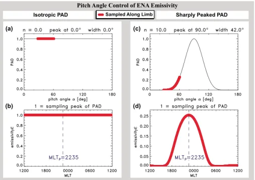
In this section we demonstrate how sharply peaked, anisotropic ENA pitch angle distributions control LAE emissivity. Figure 3 shows two hypothetical PADs, one isotropic (Figure 3a) and one peaked at 90∘ (Figure 3c), both normalized to unity. For convenience, we use the simple function sinn𝛼 for the PAD, with n = 0 giving
an isotropic distribution and n> 0 (in this example, n = 10) describing the anisotropic case. It is assumed that the PADs do not vary with geophysical location (MLT, latitude). This simplifying assumption is used in our example to demonstrate the effect of anisotropic PAD on LAE emissivity. The PA control of ENA emissivity would be qualitatively similar for PADs that vary with MLT and latitude. However, we note that the assumption of PA uniformity is also consistent with the model results of section 3.1. (In section 3.1 we discuss the possible validity and consequences of this assumption.)
The example values of𝛼 sampled by the TWINS imager (with the viewing geometry depicted in Figure 2) are indicated by the bold red curves. Figures 3b and 3d plot the theoretical LAE emissivity (𝜀) for each of the two hypothetical PADs. The emissivity is herein defined solely in terms of the PAD function. For a sampled value of pitch angle,𝛼i, the emissivity𝜀iis simply the value of the PAD function at that pitch angle. Using a normalized
PAD function (as in Figure 3) means that the emissivity is likewise normalized, with unity indicating that TWINS limb pixels sample the peak of the PAD. Note that our dimensionless, normalized emissivity differs in definition from that of Bazell et al. [2010], which bears the units of differential flux.
For the isotropic case, there is no MLT dependence, i.e.,𝜀 = 1 along the entire limb even though TWINS only samples a finite range of𝛼. For the anisotropic case, however, the incomplete pitch angle sampling means that TWINS does not capture the PAD peak, and𝜀 < 1. The emissivity is sharply peaked at MLTP, 12 MLT h away
from the TWINS location, and for the assumed viewing geometry and n = 10 distribution, the peak value is𝜀 = 0.25. Thus, even the brightest LAE pixels may represent only a fraction of the peak of the distribution. Moreover, for the case of anisotropic PAD, the LAE has a strong MLT dependence along the limb that would be evident even in the hypothetical case of ion precipitation that is uniformly distributed in MLT. This simple model predicts a steep drop in emissivity with MLT distance from the peak, with the half maximum location ±3 MLT h from the peak. The emissivity falls from its peak value of𝜀 = 0.25 at MLTPto𝜀 = 0.07 at 1800 MLT or 28% of the peak.
Figure 3. Emissivity (𝜀) dependence on local pitch angle along LAE limb. (a) Isotropic PAD (normalized). Red points: sampling along the limb. (b) Normalized emissivity for isotropic PAD. (c) Anisotropicsinn𝛼PAD. (d) Emissivity for
anisotropic PAD. Viewing geometry does not sample PAD peak.
To obtain closed-form, analytical solutions, we have (following G13) assumed that each pixel LOS vector a intersects the LAE region at a single point. In reality, each LOS cuts through a thin (few hundred kilometers) spherical shell of LAE source emissions. Moreover, each pixel subtends a range of limb latitude values. There-fore, in reality each TWINS pixel can include a range of local pitch angle, although that range is limited by the physical size of the ENA source region, which is smaller than the pixel. The effect of discrete (finite-size) pixels is discussed in section 2.4.
2.4. Limb Sampling With Discrete, Offset Pixels 2.4.1. Spatial Discretization
The analysis of sections 2.1–2.3 assumes ideal TWINS pixels. By “ideal pixels” we mean pixels that sample the exact assumed location of the LAE source. In reality, TWINS pixels are of finite angular width (nominally, 4∘; cf. section 5.2 for optional 1∘ pixels), and each LAE pixel center is offset from the limb by a viewing angle Δ𝜔i
that is generally in the range 0∘ to 3∘.
Limb sampling with discrete, offset pixels is depicted in Figure 4, which plots latitude (Λ) and pitch angle (𝛼) versus MLT, as sampled from the TWINS 2 location depicted in Figure 2. Three assumed locations are shown as follows: the exact limb (blue curve), the actual pixels (red circles), and average offset limb (red curve). 1. The blue curve is the Λ (or𝛼) sampled along the exact geometric location of the LAE limb at r = RE+ h.
2. The red points give the centers of the actual TWINS pixels, which are offset from the exact limb. The individual pixel offsets Δ𝜔ican translate to excursions of tens of degrees in both Λ and𝛼.
3. The red curve shows Λ (or𝛼) along an arc displaced from the true limb by the average (over all pixels) offset ⟨Δ𝜔i⟩ = 1.2∘.
4. The (asymmetrical) error bars indicate the uncertainty associated with 4∘ wide pixels. Specifically, each error bar is calculated by applying a ±2∘ shift to each of the (actual) pixel centers. In our formulation −2∘ is closer to the nadir line, and +2∘ is closer to the limb. On the limb side, the error bars are bounded by the exact limb (blue curve).
Note that in Figure 4a the pixel centers (red points) are higher in latitude than the exact limb. This results directly from our limb identification algorithm, which only selects pixels whose centers are at or within the exact limb.
The viewing geometry of a pixel is illustrated in Figure 4c. The center of pixel i intersects the limb at latitude Λiand samples pitch angle𝛼i. The pixel edge that crosses the limb at lower latitude ΛA(i.e., on the left in
Figure 4. Sampling of LAE limb by discrete, offset TWINS pixels. (a) Limb latitude sampled by actual pixels (black error
bars), exact limb (blue), and average offset pixels (red curve). (b) Pitch angle. (c) Viewing geometry of discrete TWINS pixel that samples range of latitudes and pitch angles. (d) Ion pitch angle versus mirror altitude at four selected altitudes spanning the thick target region (200–800 km).
the diagram) samples pitch angle𝛼A. The higher-latitude (toward nadir) pixel edge samples𝛼B. From Figure 4
it is evident that a discrete pixel samples a range of values of pitch angle𝛼. Consequently, the geometrical emissivity of pixel i, spanning [𝛼A, 𝛼B], must be calculated as a definite integral:
𝜀i= ∫𝛼B 𝛼A d𝛼 g(𝛼) f(𝛼) ∫𝛼B 𝛼A d𝛼 g(𝛼) . (1)
Here f is the local pitch angle distribution, and g is a weighting function that accounts for possible latitudi-nal dependence of the ion precipitation. As shown in Figure 4c, the latitude range spanned by the TWINS pixel samples a range of pitch angles [𝛼A, 𝛼B]. An inhomogeneous latitudinal dependence of the ions means
that some pitch angles within the pixel are weighted more than the others. Thus, the nonuniform (in latitude) case translates into inhomogeneous sampling of pitch angles within the interval [𝛼A, 𝛼B]. For no spatial dependence, g = 1 and 𝜀i= 1 𝛼B−𝛼A∫ 𝛼B 𝛼A d𝛼 f(𝛼). (2)
Bazell et al. [2010] defined the emissivity as the LAE intensity from a source region that is uniform in both latitude and local time; by this definition we should use g = 1. However, TWINS pixels cannot resolve the latitudinal dependence of the ion precipitation region. The use of g≠ 1 is a potential means of factoring out this unresolvable latitudinal dependence, to extract an emissivity dependent purely on MLT (cf. section 4.1.2). Here we are focusing on the subpixel latitudinal dependence but are saying nothing about the subpixel MLT dependence. This rationale for this focus is that for TWINS pixels the latitude sampling is much coarser (tens of degrees) than the MLT sampling (0.2–0.5 h), as shown in Figure 9b. More is said about this topic in section 6. From Figure 4 it is evident that limb pixels can sample pitch angles greater than 90∘. Although we do not have an analytical model of the thick target region, the motion of ions can serve as a helpful conceptual guide.
Ions with𝛼 >90∘ must have mirrored below the ENA limb, and it is reasonable to question whether particles at these sublimb mirror point altitudes are likely to be lost. Figure 4d shows pitch angle versus mirror altitude (for a dipole field line at L = 4) at four selected altitudes spanning the thick target region (200–800 km). For example, at 400 km (blue curve), ions at𝛼 = 107∘ mirror at 200 km (i.e., at the bottom of the thick target region). The farther from 90∘ the pitch angle is at a given altitude, the lower down the mirror point is. With decreasing ion mirror altitude, the likelihood of being lost increases. Thus, in the altitude range of the thick target region (200–800 km), there is a limited range of pitch angles for which upward moving ENAs can be produced. From Figure 4d, upward moving ions in the 200–800 km range have an approximate pitch angle range of 90∘< 𝛼 < 120∘, which compares well with simulation results for emergent ENAs (cf. section 3).
2.4.2. Energy Discretization
Another discretization effect arises from the finite-size energy bins for TWINS fluxes. The nominal TWINS energy band pass [e.g., Goldstein et al., 2013] is 100% wide; i.e., each energy bin Ejintegrates ENA counts from
Ej− 0.5Ejto Ej+ 0.5Ej. Thus, the 1 keV bin spans 0.5–1.5 keV, the 4 keV bin spans 2–6 keV, and so on through the 50 keV bin (25–75 keV). Based on kinetic simulations (cf. section 3.2), we find that the pitch angle dis-tribution of emergent ENAs depends on energy. Thus, the finite energy band-pass ΔEjcan sample a range
of different energy-dependent pitch angle distributions F(𝛼, E). To account for this finite ΔEj, we define an
energy-integrated PAD: f (𝛼) = ∫ EB EA J(E)F(𝛼, E) dE ∫EB EA J(E) dE , (3)
where [EA, EB] = [0.5Ej, 1.5Ej]. In equation (3) each integrand is weighted by the factor J(E), the flux-versus-energy spectrum (cf. section 3.2.2). Here J(E) is defined as the local ENA flux (at the source). In section 3.2.2 we estimate this quantity using the TWINS-observed ENA flux spectrum.
3. Estimate of ENA Pitch Angle
In the previous section we motivated our study by demonstrating that emissivity is a major effect for LAEs and that it is strongly controlled by the local PADs. Therefore, to quantify the emissivity requires a model of the low-altitude ENA pitch angle distribution. In this section we construct a very basic analytical model for PAD, which depends only on ENA energy (E), based on a computer simulation of the thick target region. Appendix B discusses observations of LAE pitch angle distributions by Søraas and Aarsnes [1996] and Pollock et al. [2009].
3.1. Computer Simulation of ENA Production 3.1.1. Description of the Code
To estimate the PADs of low-altitude ENAs, we use a direct Monte Carlo computer simulation code [Hubert et al., 2001; Gérard et al., 2000; Strickland et al., 1993]. Though primarily used to estimate the Doppler-shifted Lyman alpha emissions from ENAs produced in the proton aurora [Galand et al., 1998; Hubert et al., 2001; Gérard et al., 2001], the code is also suitable for studying the characteristics of the emergent ENAs themselves. The simulation solves the kinetic equations for electrons, protons, and hydrogen ENAs interacting with ther-mospheric neutrals (O, O2, and N2) in the auroral region and tracks their PADs as they propagate through the
thick target region. The velocity vector redistribution of incident (precipitating) protons includes treatment of magnetic mirroring in a dipole field [Galand et al., 1998; Galand and Richmond, 1999], geometric spreading caused by convergent (or divergent) magnetic field lines, and collisions. Our version of the code is modified to output results at nine TWINS energy channels: (1, 4, 8, 12, 16, 20, 25, 30, 50) keV. This modification to out-put selected energies is a retrofit to a legacy (unsupported) Fortran code. Although in principle the Monte Carlo simulation can be used to replace the TTA correction factor (used later; cf. equation (8), section 5), this additional retrofit is reserved for a future study.
The Monte Carlo simulation offers a very powerful way to study LAEs. This method deserves more atten-tion and discussion than can fit within the scope of this paper, which treats the simulaatten-tion as a “black box.” Although we ran the simulation for different incident energies (cf. section 3.1.3), we have not yet performed any systematic studies of the variation of the results as a function of inputs or models (e.g., kappa value and exospheric density model). Such testing enables estimation of errors as a function of physical param-eters. Lacking this more rigorous testing, our error analysis (below) is limited to calculating the standard deviation of the mean value of each ensemble of simulations. Much more can be said about this method [Strickland et al., 1993; Gérard et al., 2000; Hubert et al., 2001], and much more can be done with this code in future studies.
3.1.2. Model Inputs
The model requires several input parameters: date and time, the F10.7solar index, the AP index, and
pro-ton incident energy flux (𝜙I) and energy (EI). Continuing to use our case study of 1130 UT on 6 April 2010 (Figure 1), we chose F10.7= 77.7 and AP = 40 (from OMNIWeb). Hubert et al. [2001] used a statistical model to specify their incident (downward) proton energy flux𝜙I. We chose the arbitrary value𝜙I= 1 erg cm−2s−1,
uni-formly applied at all grid locations (see description of grid below), because our emissivity function (defined as the fraction of the PAD peak) does not depend on absolute flux values. The incident proton spectrum is a kappa distribution with 𝜅 = 3.5. The input parameter EI sets the kappa function’s peak energy at
E = EI[1 − 3∕(2𝜅)].
3.1.3. Simulation Runs and Grid
We ran the simulation for three values of incident proton energy: EI = [1, 12, 50] keV. The computation time
increases with EI: approximately [1 h, 2 h, 5 h] per grid point at [1, 12, 50] keV, using a MacBook Pro (2.33 GHz
processor, 8 GB of RAM). We used a much coarser spatial grid for the 12 keV and 50 keV runs, in part because of this increased computational expense but also because all runs showed only a weak dependence on geo-graphic location, as is discussed in section 3.1.4. The selected spatial domain is a grid of geogeo-graphic latitude and longitude (GLON) versus altitude (between 126 km and 668 km). We chose our grid to span 40∘ –80∘ of latitude and 360∘ of longitude. For the 1 keV run, we used latitude-longitude spacing of 4∘ × 15∘ with over-lap at 180∘ longitude, i.e., an 11 by 25 grid (275 grid points total). For the 12 keV and 50 keV runs, we used 10∘ × 45∘ spacing, i.e., a 5 by 9 grid (45 grid points). In total, these three runs took approximately 25 days of computation. The code is not parallelized.
3.1.4. Simulation Results
The simulation results are shown in Figure 5. Figures 5a, 5d, and 5g show the flux of emergent ENAs at 668 km altitude, versus latitude and longitude. The 2-D emergent ENA flux is relatively uniform with only random variations versus location: the standard deviation of the (1 keV, 12 keV, and 50 keV) flux is (9%, 20%, and 20%), as perhaps expected given the uniform incident energy flux𝜙I. Note that these deviations are
pro-portional to N−0.5
G , where NGis the number of grid points. Figures 5c, 5f, and 5i quantify the ENA pitch angle
distributions at 668 km, as follows. At each grid point, the code yields a pitch angle distribution at 4∘ PA res-olution. For each grid point we fit a spline of the emergent PAD to the functionn̄𝛼. Here ̄𝛼 ≡ (𝛼 − 𝛼
0+𝜋∕2),
where the𝛼0parameter allows for a PAD whose peak is not at 90∘. Figures 5c, 5f, and 5i are 2-D plots of the value of n for this fit. These are high values of n, corresponding to highly perpendicular PADs, consis-tent with ENAs produced near ion mirror points. Each plot is annotated with the mean values of n and𝛼0 and their standard deviations. As with the fluxes, over the 2-D grid the n value has no clear spatial depen-dence, with a standard deviation of (17%, 35%, and 36%) at (1 keV, 12 keV, and 50 keV). The PAD peak location 𝛼0is even more uniform, with a standard deviation of≤1% at all energies. This relatively weak (and
ran-dom) variation of emergent ENA PADs suggests that our model (cf. section 3.2) need not depend on latitude or MLT.
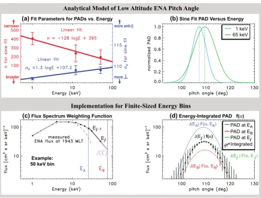
By inspection of Figures 5c, 5f, and 5i, the PAD peak location𝛼0has at most a mild energy dependence: 𝛼0varies by less than 2% as energy increases from 1 keV to 50 keV. To test whether this small𝛼0variation
is dependent on the spatial grid, we rebinned the 1 keV run to 8∘ × 45∘ and found no change in𝛼0. In contrast, the parameter n does have an energy dependence, falling by nearly 50% over the same energy range. This energy dependence is discussed below. At all energies, the large n values indicate PADs that are very sharply peaked (anisotropic). Figures 5b, 5e, and 5h plot each model run’s fluxes (versus PA), for all grid points on the same axes. The blue dots give the mean values at each pitch angle, and the red curve is a sinn̄𝛼 fit to the entire data set. The plot is annotated with the fit parameters n and 𝛼0, which are
compara-ble to the mean values from the 2-D plots. The energy dependence of n is evident in these PAD plots: as energy increases, n falls by roughly 50%, and the simulated PAD becomes slightly broader. Between 1 keV and 50 keV, n falls from about 400 to 200, with corresponding full width half maxima increasing from 6.7∘ to 9.5∘, i.e., by about 2.8∘. It is reasonable to question the significance of the differences in the low-energy and high-energy PADs, which would possibly be difficult to observe in real particle distributions. In this paper we choose to use the simulation’s energy-dependent n to create an energy-dependent model of ENA PADs, in part because the broadening of the PAD with energy is consistent with theoretical expectations, as discussed in section 3.2. An alternate approach (which we do not herein choose) would be to discard the simulation’s energy dependence of n and combine the results from all energies into a single average value of n.
Figure 5. Output of Monte Carlo simulation for[1, 12, 50]keV. (a, d, and g) Flux at 668 km altitude, geographic coordinates. (b, e, and h) PADs of all grid points withsinn̄𝛼fit. (c, f, and i) Two-dimensional maps ofnfit parameter. Black lines in color bar show meannand standard deviation.
3.2. PAD Model Versus Energy
3.2.1. Analytical Model of LAE Pitch Angle
In this section we compile the computer simulation results (section 3.1) to obtain a simple model of ENA pitch angle. Our model assumes that ENA pitch angle distributions are spatially uniform, i.e., depend only on the energy of the emergent ENAs and not on latitude or MLT. It is worth briefly discussing the validity and signifi-cance of this approximation, which is based on the simulation output that (to zeroth order) does not contain a systematic geographical dependence. In nature, any spatial dependence would result from asymmetries in the neutral exospheric density (and thus collision cross sections). Larger exospheric densities would cause higher ENA fluxes and more sharply peaked PADs. The Monte Carlo simulation estimates exospheric oxygen density using the MSIS86 model [Hedin, 1987, 1991], which has a factor of ∼2 day-night density asymmetry, at 400 km altitude and for latitudes between 40∘ and 80∘. For the simulation results of section 3.1, the dayside sector is centered at ∼7.5∘ GLON. There does not appear to be a systematic dayside asymmetry in ENA flux (Figures 5a, 5d, and 5g) or in ENA pitch angle (Figures 5c, 5f, and 5i). Although there is the hint of an asym-metry (favoring ∼0∘ GLON) in the PAD for 12 keV (Figure 5f ), because this asymasym-metry does not appear in the 1 keV or 50 keV distributions, it can be attributed to random fluctuations. Thus, despite the ∼factor-of-2 diur-nal asymmetry in the MSIS86 density model, the simulation output has no systematic (across all energies) dayside asymmetry. We leave it for a future study to quantify the effect of exospheric density asymmetries larger than the factor of ∼2 in the MSIS86 model.
To parameterize our model, we continue using the sinn̄𝛼 function. Our ENA PAD model parameters n and 𝛼
0
Figure 6. Model of ENA PAD based on simulation output of Figure 5. (a) Model fit parameters. (b) Model PAD plotted at
[1, 65]keV. (c) Determination ofJ(E)for 50 keV pixel at 1943 MLT. (d) Resulting energy-integrated PAD (black) and single-energy PADs at(EA, Ej, EB).
Figures 5b, 5e, and 5h, and the error bars on these values are their standard deviations (same as Figures 5c, 5f, and 5i). The red and blue lines are linear fits to n and𝛼0(respectively) versus log E. The model n maintains the
energy dependence noted earlier, falling by 59% (from 395 to 163) between 1 keV and 65 keV. On the other hand, the model𝛼0increases by only 2% over the same energy range, from 107∘ to 109∘. The progression
(with energy) from more narrow PADs located at smaller𝛼0to slightly broader PADs at larger𝛼 is illustrated in
Figure 6b.
While a particle is an ENA, it travels ballistically across magnetic field lines. Because the Earth’s magnetic field diverges with increasing altitude, an ENA with 90∘ pitch angle will arrive at a neighboring field line with a larger component of upward field-aligned motion, which for Northern Hemisphere LAEs means>90∘ pitch angle. When the ENA is reionized, this>90∘ PA translates into an upward (antiparallel) ion bounce motion. Multiple successive neutralization and ionization interactions thus gradually convert a mirroring ion into an emergent ENA with𝛼 >90∘ [Galand and Richmond, 1999] (K. LLera et al., submitted manuscript, 2015]. With this process in mind, the trends in model n and𝛼0are consistent with expected particle behavior in the thick target region [Galand et al., 1998], where a particle experiences numerous charge exchange and strip-ping (i.e., neutralization and ionization) interactions that gradually convert a mirroring ion into an emergent ENA with𝛼 >90∘. The stripping collisional cross section increases with E up to about 60 keV [Basu et al., 1987; Goldstein et al., 2013], meaning that more energetic particles have a shorter mean free path; these particles will undergo more stripping collisions and therefore should have broader PADs (i.e., lower values of n). More ener-getic particles will travel farther upward along the field while they are ions, both because the charge exchange cross section decreases with ion energy and more energetic ions travel faster. These hotter particles increase their PA at a slightly higher rate (per kilometer of altitude) than colder particles. Thus, with increasing E, the PAD broadens, and the PAD peak location𝛼0migrates farther from 90∘, in the antiparallel (upward) direction.
3.2.2. Implementation for Finite Energy Bins
To account for the energy discretization by finite-size TWINS energy bins, we use equation (3) to calculate the energy-integrated PAD as
f (𝛼) = f−1 0 ∫
EB EA
where ̄𝛼(E) = 𝛼 − 𝛼0(E) +𝜋∕2 and f0= ∫ J(E) dE (integrated from EAto EB). The integration limits span the 100% wide energy bin centered at Ej: [EA, EB] = [0.5, 1.5]Ej. The energy-dependent values of n(E) and𝛼0(E)
are calculated using the analytical PAD model of section 3.2.1.
In equation (4) the integrand is weighted by the local ENA flux versus energy J(E). We estimate this spectral weighting function as a two-point linear fit (in log-log space) to the observed (per-pixel) energy spectrum. At each energy bin (Ej) and pixel the fit is constrained by two-point arrays of flux (J) versus energy (E) at or
adjacent to Ej. For energy Ej, this fit is
J(E) = Jj−1 ( E Ej−1 )mj , (5) where mj= log(Jj∕Jj−1 ) log(Ej∕Ej−1) . (6)
For j = 0, these two formulas require the substitution j→ j + 1. An example of this fitting procedure is shown in Figure 6c. Plotted in black is the ENA flux spectrum measured by TWINS 2 at 1943 MLT and 1131–1145 UT on 6 April 2010 (cf. Figure 1). For reference, the dashed line shows a Maxwellian (kT = 7 keV). For the energy bin centered at 50 keV, [Ej−1, Ej] = [30, 50] keV and [Jj−1, Jj] = [72, 32] (cm2sr s keV)−1. Using these values
in equation (5) yields the fit J(E) plotted in lavender, which spans the entire 25–75 keV bin. A different such J(E) is calculated for each pixel along the limb, since the LAE spectrum is observed to vary with MLT [Goldstein et al., 2013].
There is a technical complication associated with using the TWINS-observed per-pixel ENA flux to estimate the local ENA flux J(E). The observed flux Jobsis itself the product of the local ENA flux times the local pitch angle
distribution, averaged over the energy bin, i.e., Jobs∝∫EB
EA J(E)f (𝛼i, E) dE. In general, this would lead to “double
counting” of the PAD in the integrals of (4). However, one can easily show that for steeply rising or falling spectra (e.g., Figure 6c) the observed flux versus energy is dominated by the local flux spectrum, not the PAD variation with energy. In this case, the per-pixel PAD may be approximated by its energy bin-averaged value fj.
In the example of Figure 6c, the difference between calculating Jobswith an energy-dependent PAD versus
the bin-averaged PAD is<1%. Therefore, Jobs≈ fjJ(E), and the PAD dependence of Jobscan be factored out of
both numerator and denominator of (4). In the case of a relatively flat spectrum, for which the approximation fails, one can revert to the single-energy PAD.
With the spectral weighting function determined, the integral in (4) can be calculated. We use a simple rect-angular approximation with 51 log-spaced energy steps spanning [EA, EB]. An example for the 50 keV bin is shown in Figure 6d. Each solid curve (blue, red, and green) shows the single-energy PAD F(𝛼, E), scaled by the ENA flux at that energy. That is, each solid curve is a plot of the integrand of (4) at a different value of energy E. The blue and red curves show the scaled PADs at the endpoints (EAand EB) of the numerical
integration. The green curve is the scaled PAD at Ej = 50 keV, the center of the energy bin. The black dots
show the energy-integrated PAD obtained from equation (4). The error bars are obtained via error propa-gation of the standard deviation of the analytical PAD model (Figure 6a). For this particular example, the energy-integrated PAD (black dots) is not significantly different than the single-energy PAD (green curve) that would have been obtained by simply applying equation (4) to the energy bin center Ej. In the general case,
how different the integrated PAD is depends on the per-pixel J(E) spectrum and the energy bin. The energy integration is the correct method to account for the full range of energy-dependent PADs captured by a TWINS pixel.
4. TWINS Emissivity Estimate
In section 2 we showed how the TWINS viewing geometry samples a limited range of ENA pitch angles along the limb. For anisotropic PAD and a given viewing geometry, this means that the LAE emissivity𝜀 depends strongly on MLT along the limb. In section 3 we used simulations to formulate an energy-dependent model for the PAD, which is anisotropic and centered at pitch angles slightly above 90∘, as expected. In this section we use the preceding analysis to estimate𝜀 for our case study TWINS 2 image of Figure 1.
Figure 7. Emissivity (𝜀) curves, TWINS 2, 1131–1145 UT, 6 April 2010. (a) Pixel-integrated𝜀forg = 1at exact limb (blue), actual pixels (black), and average offset limb (red). Lavender curve: normalized ENA curvefENA.𝜀∕fENA(bottom). (b) Pixel-integrated𝜀forg≠ 1. (c) Single-value𝜀.
4.1. Calculated Emissivity
To estimate LAE emissivity for the 50 keV TWINS 2 image from 1131 to 1145 UT on 6 April 2010, we perform nine different computations, all using energy-integrated PADs as in section 3.2.2. The results of these different calculations are compared in section 4.2.1 to determine the optimum method. For all emissivity values, error bars are obtained via error propagation of the standard deviation of the analytical PAD model (Figure 6a). The results are shown in Figure 7 and described in the following text.
4.1.1. Pixel-Integrated, Uniform g(𝜶): Three Versions
First, we assume that ion precipitation is uniform in latitude (consistent with the emissivity definition of Bazell et al. [2010]); i.e., we assume g = 1 and use equation (2). The integration uses a five-point Newton-Cotes algorithm (the “int_tabulated” function in Interactive Data Language). The resultant pixel-integrated emissiv-ity curves are plotted in Figure 7a, for three different assumed limb pixel locations: exact limb (blue), actual pixels (black, open circles), and average offset pixels (red), as described in section 2.4.1. The blue circles are for pixels whose fields of view span ±2∘ from the exact geometric limb. The black circles result from integra-tion across the actual pixel fields of view, using the individual pixel offsets Δ𝜔i. Note that there are no filled
black circles, although there are a handful of instances of open black circles plotted on top of blue dots. The red circles are for pixels within ±2∘ of the all-pixel average offset (⟨Δ𝜔i⟩ = 1.2∘) limb. The lavender curve is
the observed 50 keV ENA flux along the limb, normalized to unity for comparison with the emissivity curves (section 4.1.4).
These three pixel-integrated, g = 1 emissivity curves are all similar to each other in general shape and magnitude. The red and blue curves rise more or less smoothly to a broad peak centered roughly at MLTP= 2235 MLT. The black circles follow this same general shape, but with more scatter associated with the offsets of individual pixels. In the range 1700–0300 MLT, the blue and red curves agree within their error bars; outside of this core MLT range the blue curve diverges steeply downward from the red curve. In this same core MLT range, the actual pixel points (open black circles) also generally agree with the other two curves, with two exceptions at about 1800 MLT and 2200 MLT. The explanation for the general agreement among the three different curves is that despite the differences in the assumed pixel center locations, the 4∘ pixel fields of view are broad enough to result in significant overlap of the integration limits for the three methods.
Figure 8. Emissivity-corrected ENA fluxes using𝜀curves of Figure 7. Yellow line: plot range of Figures 8a and 8b.
The presence of a broad peak centered at MLTPis predicted by our simple, single-point emissivity model
(sampled at the exact limb) of Figure 3d. However, in contrast to the simple model, the emissivity curve using the finite-pixel integration formula of equation (1) has a much more gradual drop in emissivity with MLT dis-tance from the peak. The simple model predicts the emissivity at 1800 MLT to be 28% of the peak at MLTP (cf. section 2.3). The pixel-integrated emissivity at 1800 MLT is 82% (or 88%) of the value at MLTPfor the blue (or red) curve.
4.1.2. Pixel-Integrated, Nonuniform g(𝜶): Three Versions
The TWINS 4∘ pixels span tens of degrees of geophysical latitude, a range much larger than that of the ion precipitation. If the ion distribution versus latitude is known, it may be factored out to yield an emissivity curve that depends solely on MLT. Lacking this information, for this study we derived an ad hoc empirical model of ion precipitation based on the statistical study of Hardy et al. [1989], as described in Appendix A. We set g = G(𝛼, MLT), where the latter function is that of equation (A4), but normalized and mapped to a corresponding distribution in sampled pitch angle𝛼 for the span of each finite-size pixel. With nonuniform g specified, we perform the integration of equation (1). In Figure 7b we plot emissivities along the exact limb (blue), actual pixels (black), and average offset pixels (red). As was the case for the g = 1 curves in Figure 7a, the three g≠ 1 curves of Figure 7b agree within their error bars in a core MLT range, in this case 1900–0100 MLT. The red and black curves agree with each other at all MLTs. All three curves have a local minimum at MLTP
that results from the fact that those TWINS limb pixels sample latitudes above the main precipitation oval (cf. Appendix A). The lavender curve does not have this local minimum, most likely because either the actual precipitation oval spans a slightly different latitude range than the model or the high-latitude boundary of the oval is less well defined than the model.
4.1.3. Single-Value Emissivity: Three Versions
Instead of integrating over the full 4∘ field of view of each pixel, we sample the PAD at a single location Λi. The weighting function is then g =𝛿(𝛼−𝛼i), and equation (1) reduces to𝜀i= f (𝛼i), i.e., the single-point (0 pixel size) case of section 2.3. The results are plotted in Figure 7c. The average offset emissivity curve (red points) is qualitatively similar to the g = 1 pixel-integrated curves (Figure 7a), with a broad peak centered roughly at MLTP, although the drop with MLT distance from the peak is comparatively steep. There are no blue points
plotted; the exact limb values are all approximately zero (𝜀i < 10−29) because the values of𝛼 sampled are
≤60∘ (cf. Figure 4b), far outside the range of 𝛼 for which the 50 keV PAD—peaked at 109∘ —is nonnegligible. The very large degree of scatter in the actual pixel emissivities (black circles) results from the variability in the individual pixel offsets (Figure 4b), which produces a pixel-to-pixel randomness in the particular values of 𝛼 sampled. The scatter is such that roughly half the actual pixel emissivities fall outside the plot range. This randomness is smoothed out for the finite-pixel emissivities (Figures 7a and 7b) that each sample a larger range of𝛼, leading to significant overlap of the various ∫ d𝛼 integrations.
4.1.4. Shape Comparisons: ENA Versus Emissivity
If the modeled emissivity (𝜀) is accurate, and if the MLT dependence of the observed ENA flux is caused by viewing geometry alone, then the𝜀 function should reproduce the global shape of the ENA flux versus MLT curve.
In this section we compare the shapes of the computed emissivities with that of the observed 50 keV ENA flux versus MLT. In each plot of Figure 7, the normalized 50 keV ENA flux (fENA) is plotted in lavender. The circles give the per-pixel values, and the solid line is a cubic spline (smoothed by a 2.4 MLT hours boxcar average) to guide the eye. As a qualitative measure of agreement, the lower panels plot the ratios𝜀∕fENAfor each of
the individual curves; in these plots, the gray colored region indicates agreement to within ±50%. For the nine different computed versions of𝜀, we find a mixture of good, moderate, and poor agreement between 𝜀 and fENA:
Figure 7a. Although the pixel-integrated𝜀icurves do have a broad peak at MLTP, they exhibit a much milder
dependence on MLT than fENAin the range 1700–0300 MLT. Only the exact limb (blue) emissivity shows some
level of agreement with fENA, but only below 1700 MLT and above 0300 MLT.
Figure 7b. For all three𝜀icurves there are local minima at MLTP, in contrast with the broad peak (centered at
MLTP) in fENA. As noted above, this discrepancy may be caused by differences between the model and actual precipitation ovals. For local times 1600–1900 MLT the slopes of the red and black curves follow that of fENA, although the values of𝜀 exceed that of the normalized ENA curve fENA.
Figure 7c. The two plotted single-point𝜀 curves show two dramatically different levels of agreement with fENA. The enormous scatter in the actual pixel emissivities (black circles) disagrees strongly with the relatively
smooth fENAcurve. On the other hand, the shape of the average offset (red) curve agrees quite well with
fENAfor 1900–2300 MLT. As noted above, the exact limb emissivities (blue points) were all negligible and are
not plotted.
The closest shape agreement seems to be for the single-point average offset (red) emissivity curve; however, as will be discussed in section 4.2, this red curve produces corrected ENA fluxes that are unrealistically high at some MLTs.
Based on these𝜀-to-fENAshape comparisons, we conclude that either the observed ENA flux’s MLT
depen-dence is not entirely caused by viewing geometry or our simple calculation is too crude to fully capture the observed emissivity versus MLT. The former possibility appears to be unverifiable without more empirical information. The latter possibility, if true, suggests that because emergent ENA pitch angle distributions are so sharply peaked, uncertainties in our method can produce very large variations in𝜀. These uncertainties include (1) per-pixel knowledge of the latitude (and thus, the sampled𝛼) of the source region and (2) errors in the analytical PAD model. Latitude uncertainty is unavoidable, as discussed earlier, and our attempt to mitigate it via a nonuniform g(𝛼) achieved reasonable agreement only in a limited MLT range. Another way to minimize latitude uncertainty is to use 1∘ pixel images (cf. section 5.2). Model error is likewise inevitable because of the shortage of published observations of the PADs of emergent ENAs.
4.2. Corrected ENA Flux
The emissivity herein represents the fraction of the PAD peak that is sampled by a TWINS pixel. To correct the ENA flux (JENA) for this viewing geometry effect means dividing it by𝜀:
Jcorr= JENA[𝜀]−1. (7)
Figure 8 plots values of Jcorralong the exact limb (blue), actual pixels (black), and average offset pixels (red), for the pixel-integrated and single-valued emissivities. The uncorrected ENA flux is plotted in lavender. We next compare these several different calculations of Jcorr to choose a single method for further analy-sis. In section 4.1.4 we compared the shapes of𝜀(MLT) curves with normalized ENA flux curves. This purely shape-based comparison was performed under the assumption that the observed MLT dependence of ENA flux is at least in part caused by emissivity. In this section we are calculating corrected ENA fluxes; i.e., we are attempting to use the estimated emissivity curves to factor out the emissivity dependence. In principle, Jcorrshould be the global ENA distribution (along the limb) without viewing geometry effects. In practice (see below), this correction is of course limited and imperfect. Therefore, in the remainder of this section we merely discuss whether the corrected curves appear to be physically reasonable and/or consistent with each other. In section 5 we attempt to judge the accuracy of Jcorrby converting it to ion flux and comparing with NOAA data.
4.2.1. Pixel-Integrated Jcorr
The pixel-integrated Jcorrcurves are found in Figures 8a and 8b, respectively, for the uniform (g = 1) and nonuniform (g≠ 1) PAD weighting functions. The group of three g = 1 (or g ≠ 1) curves all agree within their error bars in the range 1800–0300 MLT (or 1900–0100 MLT), as expected from the agreement found for the corresponding groups of emissivity curves (Figure 7). The two groups of three Jcorrcurves are also
compara-ble: except for a factor of ∼2 difference in magnitude, the g = 1 and g≠ 1 curves are all quite similar in shape between 1900 and 0100 MLT. This agreement is somewhat surprising given the differently shaped𝜀icurves
for the uniform versus nonuniform g found in Figure 7. However, it is worth noting that the pixel-integrated emissivities all vary by less than a factor of 2 in this MLT range. The similarity of the six different Jcorrcurves is
encouraging given the large uncertainties in the emissivity calculation (section 4.1.4).
Based on the similarity between the two main variations (g = 1 and g ≠ 1) of pixel-integrated emissivity calculation, we conclude that either method is acceptable to obtain corrected ENA flux. We choose the g = 1 method for further analysis, because the g = 1 method employs an emissivity definition more consistent with that of Bazell et al. [2010] and does not require an additional empirical model (e.g., the H89 model of Appendix A). Next we consider the three different g = 1 curves (blue, black, and red), which are all quite similar in shape and magnitude. We reject the exact limb method (blue curve) because although this curve is smooth and well behaved, the exact limb pixels are displaced (on average) tens of degrees away (in both Λ and𝛼) from the actual pixels. On the other hand, even though in principle the actual pixel values (black points) should be most accurate, the scatter in these points is undesirable (and may introduce additional unquantifiable error associated with the relatively large pixel size). Therefore, we choose the g = 1 average offset method (red curve) for analysis of 4∘ images (section 5.1), to avoid pixel-to-pixel scatter from individual offsets while still placing the pixel centers in the correct locations, on average. We choose the g = 1 actual pixel method (black dots) for analysis of 1∘ images (section 5.2) because the pixel-to-pixel offset scatter is much less for the higher-resolution images (Figure 10).
4.2.2. Single-Value Method
The single-value Jcorris plotted in Figure 8c, for actual pixels (black) and average offset pixels (red). Neither of
these methods is selected for further analysis. The pixel-to-pixel scatter in the actual pixel emissivities yields variations in Jcorrthat span several orders of magnitude. Only half of the black points are included in the plot
range, which has been expanded by a factor of 2000 relative to the previous two plots. Whereas the average offset (red) curve avoids the actual pixel scatter, the central (1800–0300 MLT) correction to the ENA flux is minimal (a factor of 2 at most), and the curve contains factor-of-1000 flux increases outside of 1800– 0300 MLT that are probably unrealistic.
5. TWINS-NOAA Ion Flux Comparison
Thus far, we have determined a method to calculate Jcorr, which is the global low-altitude ENA flux with the
viewing geometry dependence at least partially factored out. In this section we extend this analysis. We use the pixel-integrated, uniform-precipitation (g = 1) emissivity (section 4) to obtain corrected TWINS ion fluxes. We compare these ion fluxes to simultaneous in situ data from NOAA 17 for two TWINS pixel sizes, 1∘ and 4∘.
5.1. Comparison Using 4∘ Pixel Image
Figure 9a plots TWINS 2 flux versus MLT from 1131 to 1145 UT on 6 April 2010. The blue circles are the emissivity-corrected ENA flux Jcorr= JENA(𝜀)−1of equation (7); dividing by𝜀 applies the emissivity correction.
The background-subtracted ENA flux JENAis obtained by estimating the background as the minimum ENA flux along the limb. The ENA flux JENAis converted to ion flux Jionusing
Jion= JENA Fc 𝜀 [ 1 +𝜎s 𝜎c ] . (8)
As in G13, Fcis a geometric, pixel size correction accounting for the fact that the vertical scale of the LAE source is smaller than the TWINS pixel [Brandt et al., 2001a; Goldstein et al., 2013]. Note that there are two different geometric corrections being performed in this paper. The emissivity correction attempts to account for the viewing geometry effect in which different pixel lines of sight sample different values of a very sharply peaked PAD. On the other hand, the pixel size correction Fcscales up the flux in an attempt to account for a source
Figure 9. TWINS-derived ion flux compared to simultaneous NOAA 17 peaks A and B (Appendix B). (a) ENA flux (blue),
uncorrected ions (gray dashed), corrected flux (colored dots, numbered), and NOAA flux (black). (b) TWINS and NOAA fluxes mapped to polar ionosphere. H89 proton oval indicated.
region smaller than the pixel; the value of Fcfor our case study is 8.16. The𝜎cand𝜎sare (respectively) the
charge exchange and stripping cross sections. The factor in square brackets is from the TTA approximation of Bazell et al. [2010] for pixel-averaged flux. We make no correction to TTA for finite-sized energy bins; however, Goldstein et al. [2013] showed that the magnitude of this correction is<3%. Note that Jion= JcorrFc
[
1 +𝜎s∕𝜎c
] . Figure 9a plots the resulting TWINS 2 ion flux values as color-coded circles. The colored error bars indicate the uncertainty arising from the standard deviation of the model PAD (cf. Figures 6a and 6d), added in quadrature to the Poisson counting errors. The thick gray line is a cubic spline fit (smoothed by a 1.2 MLT hours boxcar average) to guide the eye. Note that the average (over MLT) value of our emissivity is 0.12, so that the correc-tion (dividing by𝜀) introduces a factor of 7 increase. For reference, the uncorrected ion flux is plotted (dashed gray line). The shape of the corrected curve is not significantly different from the uncorrected curve. There is only a factor of ∼2 difference between the uncorrected ion flux (dashed line) and the corrected ENA flux (blue circles).
For comparison, NOAA 17 proton flux data are overplotted, showing the two main peaks (“A” and “B”) that occurred during 1138–1148 UT (cf. Figure B1b). To aid the comparison, Figure 9b is an ionospheric polar pro-jection (MLT versus latitude). The TWINS flux pixels are mapped onto the plot using their actual locations, and latitude edges defined as the ±2∘ viewing angle range, as in Figure 4a. The NOAA 17 proton fluxes are over-plotted along the satellite’s polar orbit trajectory. The flux color bar used for both TWINS and NOAA is the same as Figure 9a. The TWINS pixels are numbered for ease of reference.
We now compare TWINS and NOAA 17 fluxes. In Figure 9b, NOAA precipitation peak A is closest to TWINS pixel 10 (red), and NOAA peak B is closest to TWINS pixel 9 (yellow-orange). For these two conjunctions, the NOAA ion fluxes are 3 to 14 times larger than those derived from TWINS. In Figure 9a, the mean value of each NOAA peak is indicated (thick gray horizontal lines). NOAA peak A (or B) has flux 14 (or 3) times larger than that of TWINS pixel 10 (or 9). It is unsurprising that the NOAA fluxes are higher than those of TWINS. In Figure 9b, each TWINS pixel spans tens of degrees of magnetic latitude and 0.2–0.5 h in MLT. The NOAA data contain spatial structures too small to resolve with TWINS pixels. Averaged over the large area of a TWINS pixel, such smaller-scale structures are smoothed out, resulting in a lower mean flux. With this understanding, agreement in absolute flux to within an order of magnitude is encouraging. Using the full numerical calculation of LAE emissivity, Bazell et al. [2010] obtained TWINS fluxes 2 to 9 times smaller than simultaneous Defense Meteoro-logical Satellite Program (DMSP) in situ flux values. We have achieved a comparable level of agreement (factor of 3 to 14) using a simpler and less computationally expensive method.
Figure 10. TWINS limb pixels for 4∘and 1∘oversampled pixel images. (a, b) ENA image and limb pixels, 4∘image. (c, d) ENA image and limb pixels, 1∘image, avoiding jagged limb sampling.
For reference, the predicted oval from the H89 empirical model (Appendix A) is indicated by the gray shaded region, bounded by Λ = ΛP± ΔΛP. As discussed in Appendix B and evident in Figure 9b, the latitude range spanned by the two NOAA peaks (A and B) agrees with the H89 model’s prediction for the extent of the ion oval.
In our previous study of this event (G13), the lack of an emissivity estimate severely limited the MLT range of valid TWINS ion fluxes. Thus, G13 compared TWINS flux, averaged over all limb values within 20% of the global peak, to NOAA flux averaged over both peaks A and B. The NOAA “A+B” flux was 20 times larger than the TWINS all-limb-averaged flux. The new analytical estimate for𝜀, while still quite limited, has allowed an expansion of the MLT range of TWINS fluxes and thus a more direct comparison between individual pixel TWINS fluxes and individual NOAA peaks (TWINS pixel 9 with NOAA peak B and pixel 10 with peak A). Using the emissivity correction, the obtained level of agreement in absolute flux is improved by a factor of 1.4 (for peak A) to 7 (for peak B) compared to the uncorrected method.
5.2. Comparison Using 1∘ Pixel Image
The TWINS angular field of view is usually discretized into 4∘ by 4∘ pixels. Figure 10a shows a close-up view of the 4∘ TWINS 2 image from 1131 to 1145 UT on 6 April 2010. Figure 10b is the same image but showing only the limb pixels. Here limb pixels are defined as those whose centers lie within an annulus bounded r = RE+ h
(outer), and by the critical offset angle𝜔C(inner), inside of which there are no solutions to the geometrical
equations [Goldstein et al., 2013]. The limb pixels follow a jagged curve rather than a smooth one because 4∘ pixels are comparable in size to the limb curve. From an imager at 5.6 REgeocentric distance (Figure 2a), the LAE limb diameter (2a) spans 21.5∘ or 5.4 pixels across. The jagged sampling produces large scatter in the sampled latitude and pitch angle and bunching of sampled MLT values (Figure 4). MLT bunching is evident in Figure 9; e.g., there is a gap of nearly 2 MLT hours between pixels 13 and 14. As discussed in section 5.1, using 4∘ pixels means the LAE source location is uncertain by tens of degrees of latitude, and derived per-pixel ion fluxes are artificially low in comparison to in situ data.
In an attempt to mitigate latitudinal uncertainty and pixel-averaged flux reduction, we next compute emissivity-corrected ion fluxes using 1∘ pixels. To explain how 1∘ images are made requires a brief description of the instrument [McComas et al., 2009, 2012]. Each of the TWINS imagers has two collimating sensor heads, mounted on a rotating actuator that sweeps through 180∘ and back to capture ENAs in a cone-shaped field of view. Each sensor head measures incoming ENAs in two orthogonal directions: the instrument’s 1-D imaging angle𝜆 (parallel to the collimator plates) and the actuation angle 𝛽. The TWINS imagers do report 𝛽 posi-tion with 1∘ accuracy, and the direct-events imaging angle informaposi-tion can (in principle) be discretized into arbitrary-sized pixels. Thus, it is possible to create images with 1∘×1∘ pixels for count rates below the telemetry rate [Valek et al., 2010; McComas et al., 2012; Valek et al., 2013, 2014]. However, these smaller pixels oversample the instrument angular resolution in both dimensions, as follows. First, the slit camera has an angular (ver-sus𝛽 response curve that is 4∘ wide at full width at half maximum (FWHM). Second, owing to foil scattering and MCP/anode signal spreading, the imaging angle has an intrinsic, energy-dependent FWHM angular res-olution that is ∼16∘ at 1 keV and levels off to ∼7∘ at energies above ∼10 keV [Goldstein et al., 2013]. Thus, sorting ENA counts into 1∘ × 1∘ bins is an oversampling of the intrinsic𝜆 × 𝛽 instrument angular resolution, which for 50 keV ENA images is ∼ 4∘ × 7∘. What is then gained by this oversampling? The smaller𝛽 pixels
Figure 11. TWINS 2 and NOAA 17 ion flux, for higher-resolution 1∘TWINS pixels. (a) TWINS ion flux (colored dots), NOAA flux (black), spline of 1∘TWINS flux (gray), and spline of 4∘flux (gray dashed).Rion≡ Jion(1∘) ÷ Jion(4∘), showing factor of ∼2 ratio between 1900 and 2200 MLT (bottom). (b) TWINS and NOAA fluxes mapped to polar ionosphere, with H89 proton oval indicated.
more closely conform to the limb’s circular shape, reducing the jaggedness of the limb curve (see below). Oversampling an image has also been shown in some cases to slightly improve effective resolution [e.g., Fruchter and Hook, 2002; Bai et al., 2011].
Figure 10d shows the LAE limb at 1∘ resolution, with much reduced jaggedness of the sampled limb curve, and oversampling of the ENA signal in both latitude and MLT. At this higher resolution the limb annulus contains 422 pixels, as compared to the 30 pixels of the 4∘ image. Figure 11 shows ion fluxes calculated using the 1∘ image. To facilitate comparison with high-flux NOAA data obtained above 55∘ latitude, we filtered the 422 limb annulus points by retaining only points that satisfy the criterion𝜀 ≤ 0.25, resulting in 37 points between 1600 and 0100 MLT. Using 1∘ images, the individual pixel fluxes are not consistently closer to the fluxes of NOAA peaks A and B. NOAA peak A has flux 6 times larger than corresponding TWINS 1∘ pixel A (labeled in blue), a factor-of-2 improvement compared to the 4∘ pixel comparison. NOAA peak B’s flux is 7 times that of TWINS pixel B, a factor-of-2 worse comparison than the 4∘ case.
However, with the smaller 1∘ pixels, the highest (peak) derived ion fluxes are a factor of ∼2 higher than for the 4∘ pixel image, as follows. The gray solid line is a cubic spline (smoothed by a 0.8 MLT hour boxcar average) of the 1∘ flux. The gray dashed line is a spline (smoothed by 1.2 MLT hours) of the 4∘ flux, taken from Figure 9. The ratio of the 1∘ and 4∘ spline flux curves is Rion, plotted in the bottom panel. In the range 1900–2200 MLT, i.e., the region of peak flux, the mean Rionis 1.7. The highest flux values derived from 1∘ pixels are thus larger than those derived from 4∘ pixels, perhaps indicating that oversampling at 1∘ may be a slight improvement for LAE imaging at higher energies. The highest TWINS fluxes (∼104[cm2sr s keV]−1) are comparable to the
mean NOAA flux (averaged over both peaks) of ∼6000 [cm2sr s keV]−1(cf. Appendix B).
As in the previous figure, in Figure 11b the predicted oval from the H89 model is given by the gray region. The TWINS 1∘ pixels that overlap the H89 model oval have higher fluxes (that agree better with NOAA data), and the pixels fully outside the H89 oval are generally (with just a few exceptions) lower.
6. Discussion
Our result shows that it is possible to correct—at least partially—for the viewing geometry dependence of low-altitude ENA emission using a simple analytical model. Such correction requires knowledge of two attributes of the emergent ENAs: pitch angle distribution and geophysical location. There are unavoidable uncertainties in both of these quantities.


![Figure 5. Output of Monte Carlo simulation for [1 , 12 , 50] keV. (a, d, and g) Flux at 668 km altitude, geographic coordinates](https://thumb-eu.123doks.com/thumbv2/123doknet/5652674.136906/9.918.310.815.135.665/figure-output-monte-carlo-simulation-altitude-geographic-coordinates.webp)