Sélection des prédicteurs pour la mise à l'échelle des données MCG par la méthode Lasso.

(1)

Université du Québec INRS-Eau Terre Environnement

SÉLECTION DES PRÉDICTEURS POUR LA MISE

À

L'ÉCHELLE

DES DONNÉES MCG PAR LA MÉTHODE LASSO

Président du jury et examinateur interne Examinateur externe Directeur de recherche Par Dorra Hammami

Mémoire présenté pour l'obtention du grade Maître ès sciences (M.Sc.)

en sciences de l'eau

Jury d'évaluation

Erwan Gloaguen

INRS-Eau Terre Environnement

Saad Bennis

École de Technologie Supérieure

Taha B.M.J Ouarda

INRS-Eau Terre Environnement

(2)

REMERCIEMENTS

La réalisation de ce mémoire n'aurait pas pu être menée à terme sans l'aide de plusieurs personnes. J'aimerai donc remercier tous ceux qui m'ont encouragé et aidé à effectuer ce travail.

Je tiens à remercier tout d'abord mon directeur de recherche Taha Ouarda pour m'avoir accueilli dans son équipe de recherche, pour son soutien moral, pour avoir cru sans cesse en mes capacités, pour ses conseils précieux et pour l'attention qu'il m'accordait tout au long de ma maîtrise.

Un grand merci à tous les membres de l'équipe de Taha qui m'ont aidé et qui m'ont donné de leurs temps. Je tiens à remercier le professeur Fateh Chebana pour son soutien moral et pour sa croyance en mes capacités.

Je voudrai exprimer ma profonde gratitude envers ma famille, ma mère Jamila, mon père Ridha, les plus belles sœurs au monde: Abir, Fadwa et Rabaa. C'est grâce à eux que je voudrai réussir, c'est avec eux que je partage la joie d'avoir fini ce travail.

Merci à tous mes amis avec qui j'ai partagé les plus beaux moments de ma vie.

Je n'oublierais jamais de remercier la personne qui me marquera pour toute ma vie, la personne qui a toujours présenté le soutien et l'aide pour moi, merci Wejden.

Finalement, j'exprime ma gratitude envers tous les membres du jury pour avoir accepté d'évaluer ce mémoire.

(3)

RÉSUMÉ

Au cours des 10 dernières années, les techniques de réduction d'échelle (dynamiques ou statistiques) ont été largement développées afin de fournir une information sur le changement climatique à une résolution plus fine que celle fournie par les modèles climatiques globaux (MCG). Vu que la plus grande préoccupation des techniques de réduction d'échelle est de fournir l'information la plus précise possible, les analystes ont essayé de nombreuses méthodes pour améliorer la sélection des prédicteurs, étape cruciale en réduction d'échelle statistique.

Des méthodes classiques sont utilisées, telles que les méthodes de régression simple en particulier la méthode de régression pas à pas. Cependant, cette dernière présente quelques limites en traitant les problèmes de colinéarité des variables ainsi qu'en fournissant des modèles complexes difficiles à interpréter. La méthode lasso est utilisée comme une deuxième alternative. L'objectif de cette étude est la comparaison des performances d'une méthode classique de régression (régression pas à pas) et de la méthode lasso. Pour ce faire, des séries de données de 9 stations situées au sud du Québec ainsi que 25 prédicteurs, s'étalant sur la période de 1961-1990 sont exploités. Les résultats indiquent qu'en raison de ses avantages de calcul et de sa facilité d'implémentation, lasso donne de meilleurs résultats en se basant sur le coefficient de détermination et l'erreur quadratique moyenne (EQM) utilisés comme outils de comparaison des performances.

(4)

TABLE DES MATIÈRES REMERCIEMENTS ... ii RÉSUMÉ ... iii PARTIEl : SYNTHÈSE ... 1 INTRODUCTION ... 2 CHAPITRE 1 ... 5 CHAPITRE 2 ... 7 RÉFÉRENCES DE LA SYNTHÈSE ... 10

PARTIE 2: L'ARTICLE SCIENTIFIQUE ... Il Résumé en français ... 12

PREDICTOR SELECTION FOR DOWNSCALING GCM DATA WITH LEAST ABSOLUTE SHRINKAGE AND SELECTION OPERATOR ... 13

Abstract ... 14

1. Introduction and brief review ... 16

2. Theoretical background ... 18

2.1. Stepwise regression ... 18

2.2. Lasso ... 21

3. Predictor selection ... 28

4. Data set for case study ... 30

5. Results ... 31

6. Discussion and conclusions ... 35

Acknowledgments ... 38

REFERENCES ... 39

APPENDIX 1: NOTATION SECTION ... 42

TABLE LIST ... 43

FIGURE CAPTIONS ... 50

(5)

(6)

INTRODUCTION

L'estimation plausible du climat futur demeure la préoccupation ultime des hydro-météorologues. La principale source de l'information météorologique provient des modèles climatiques globaux (MCG). À cause de la résolution grossière de ces derniers, les données MCG ne peuvent pas être utilisées dans des études climatiques régionales et locales nécessitant de l'information climatique à de fines résolutions (Hessami et al. 2008). La meilleure option permettant de contourner ce problème est l'utilisation de différents modèles statistiques de mise à l'échelle permettant d'exploiter les données MCG pour des études d'impact locales. La sélection des prédicteurs est connue comme l'étape primordiale et cruciale pour la mise à l'échelle des données MCG; elle consiste à sélectionner les variables explicatives les plus pertinentes quand un certain nombre de variables indépendantes potentielles existe (Fan and Li. 2001). Elle permet de construire un meilleur modèle parmi d'autres. Les travaux de recherche, rapportés dans l'article scientifique présenté dans la partie 2 concernent l'application d'une nouvelle méthode de régression pour la sélection des prédicteurs, c'est la méthode Lasso introduite par Tibshirani (1996) ainsi qu'une ancienne méthode fréquemment utilisée (la méthode de régression pas à pas). La méthode Lasso est un modèle de régression pénalisé qui permet de minimiser la somme des carrés résiduels sous une contrainte de la forme LI (la norme LI) et donc permettant d'assigner 0 aux coefficients des variables à rejeter pendant le processus de sélection.

Dans le cas d'une situation de régression ordinaire, on considère les données suivantes

(Xi, yJ

i

=

1, 2,.··, n, avec Xi =

(xii' ... '

x_ip

Y

constituent les variables indépendantes et Yi est

(7)

la réponse de la ième observation. Les estimations par moindre carré ordinaire (MCO) sont obtenues par la minimisation de la somme des carrées résiduels (SCR) mais elles ne sont pas satisfaisantes. Deux principales raisons peuvent expliquer l'insatisfaction des analystes en utilisant les estimations par MCO: La précision des prévisions et l'interprétation des résultats. Les estimations MCO sont caractérisées par un faible biais mais une large variance ce qui peut entrainer une grande erreur dans les prévisions. Ainsi, avec un grand nombre de prédicteurs, on a toujours tendance à réduire le nombre de variables qui permet d'englober la majorité de l'information produite par toutes les variables. Deux méthodes sont principalement utilisées pour combler les lacunes de l'utilisation de la méthode MCO, c'est la régression ridge et la méthode de sélection par sous-ensembles (Tibshirani, 1996). Cependant, ces deux dernières méthodes présentent des inconvénients.

La méthode de sélection par sous-ensemble peut être considérée comme une méthode instable malgré qu'elle peut produire des modèles faciles à interpréter contrairement à la méthode ridge qui est un processus continu plus stable mais qui ne donne aucun 0 aux coefficients des variables à rejeter donc ne produit pas de modèles faciles à interpréter. La méthode Lasso proposée par Tibshirani (1996) est une méthode de régression qui permet de dépasser les inconvénients des deux méthodes précédemment évoquées (la méthode ridge et la méthode de sélection par sous-ensemble). C'est pour cette raison qu'on a décidé d'appliquer ce modèle à un jeu de données afin de vérifier sa capacité d'améliorer les résultats de sélection des prédicteurs pour la mise à l'échelle des données MCG et comparer les résultats obtenus avec d'autres obtenus en utilisant une méthode classique fréquemment utilisée qui est la méthode de régression pas à pas.

(8)

Une revue de littérature a été réalisée afin d'identifier les deux méthodes utilisées dans ce travail et la progression de leurs utilisations au cours des années. Ces deux méthodes ont été appliquées à des données de température maximale et minimale issues des observations journalières de la période 1961-1990 de 9 stations qui se situent au sud, sud-est du Québec autour du golfe St-Laurent ainsi qu'à des variables indépendantes issues des réanalyses NCEPINCAR standardisées et interpolées su la grille du MCCG3 de résolution 3.75° de longitude et de latitude se situant au dessus des stations (DAI MCCG3 prédicteurs, 2008).

Une application des deux méthodes a été réalisée, suivie d'une comparaison de leurs performances suivant deux critères qui sont l'erreur quadratique moyenne comme étant un indice englobant la variance et le carré du biais des estimations ainsi que le coefficient de détermination R2 qui est un indicateur qui permet de juger la qualité d'une régression linéaire, simple ou multiple. D'une valeur comprise entre 0 et 1, il mesure l'adéquation entre le modèle et les données observées.

Cette première partie « Synthèse» du mémoire de maîtrise contient dans le chapitre 1 la contribution de l'étudiante par rapport à d'autres articles scientifiques et l'originalité du travail effectué. Le chapitre 2 traite de la contribution de l'étudiante au sujet traité et le chapitre 3 résume les principaux résultats obtenus ainsi que les conclusions qui en découlent.

(9)

CHAPITRE 1

SITUATION DE LA CONTRIBUTION SCIENTIFIQUE PAR

RAPPORT AUX AUTRES TRAVAUX

Dans cette étude, une nouvelle méthode de régression (lasso) (Tibshirani, 1996) permettant de combler plusieurs inconvénients d'autres méthodes classiques a été utilisée pour la sélection des prédicteurs pour la mise à l'échelle des données MCG. L'implémentation de cette méthode dans la procédure de sélection des prédicteurs n'a pas, à la connaissance de l'étudiante, été tenté précédemment. Cette étude peut être considérée comme une validation de la méthode lasso, elle a comme but de tester l'utilité de la méthode par rapport à une méthode classique fréquemment utilisée dans la sélection des prédicteurs qui est la régression pas à pas. L'originalité de l'étude se manifeste clairement dans l'application d'une méthode qui n'a jamais été appliquée en hydro-climatologie.

Dans la majorité des études consultées sur l'utilisation de la méthode de régression lasso, les auteurs ont essayé de donner des explications concernant l'utilité de la méthode (e.g. Tibshirani, 1996) et de développer des algorithmes plus faciles que l'algorithme principal proposé par Tibshirani (1996) vu la nature non différentiable de la fonction à minimiser (e.g. Osborne et al. 2000a) et ceci par l'intermédiaire de plusieurs études (Schmidt,

2005). Ainsi, d'autres études ont essayé de comparer la méthode lasso à d'autres méthodes plus anciennes mais qui peuvent être considérées de la même nature (la régression pénalisée) telle que la régression Bridge (Wenjiang, 1998). De même, d'autres études ont tenté d'adapter des méthodes plus anciennes comme la régression ridge pour

(10)

avoir les mêmes avantages que la méthode lasso en termes de prévisions (Grandval et et Canu, 1999) afin d'aboutir à un nouveau modèle appelé« ridge adapté ».

Dans cette étude, on a essayé d'améliorer les performances de la sélection des prédicteurs pour la mise à l'échelle des données MCG par l'implémentation d'une nouvelle méthode qui va pallier aux inconvénients des méthodes classiques.

(11)

CHAPITRE 2

CONTRIBUTION DE L'ÉTUDIANTE

Une revue de littérature a été effectuée par l'étudiante comme étape préliminaire concernant la sélection des prédicteurs en tant qu'étape cruciale dans la procédure de mise à l'échelle des données MCG ainsi que les algorithmes résumant l'idée de la régression pas à pas, les applications de cette dernière considérée comme l'une des méthodes les plus utilisées pour l'analyse et la sélection des variables en régression linéaire tout en n'oubliant pas les limites de cette méthode. La méthode lasso a été présentée comme une alternative qui pourra contourner les limites de la régression pas à pas. L'étudiante a essayé d'identifier le développement de l'utilisation de la méthode lasso en tant que nouvelle méthode de régression permettant de retenir les bonnes caractéristiques des deux méthodes classiques, la méthode ridge et la sélection par sous ensembles qui permettent de dépasser les inconvénients de la régression par moindres carrés ordinaires. Plusieurs études mettant l'accent sur l'utilisation de cette méthode ont été présentées ainsi que d'autres traitant les différents algorithmes développés pour combler le problème de l'indifférentiabilité de la fonction à minimiser (Schmidt, 2005). Dans ces études consultées, la méthode lasso n'a pas été introduite pour la sélection des prédicteurs pour la mise à l'échelle des données MCG. Ceci est expliqué dans la section introduction et revue de littérature de l'article scientifique présenté dans la partie 2 du présent mémoire.

Après la consultation des études au cours de la revue de littérature, l'étudiante a décidé de travailler avec deux méthodes de natures différentes pour la sélection des prédicteurs pour la mise à l'échelle des données MCG qui sont la méthode lasso et la méthode de

(12)

régression pas à pas. Une description mathématique des deux méthodes a été faite comme expliqué dans la section 2 de l'article scientifique présenté dans la partie 2 de ce mémoire. L'objectif principal de cette étude était donc de comparer les performances des deux méthodes précédemment évoquées.

La méthodologie employée dans l'étude est décrite à la section 3 de l'article. L'algorithme de la méthode de l'ensemble actif proposé par Osborne et al. (2000a) a été utilisé à cause de sa facilité d'implémentation, le coût réduit des itérations et les propriétés de convergences plus rapides. Cette méthode ne nécessite ni le doublement du nombre de variables ni un nombre exponentiel de contraintes.

En outre, l'étudiante a utilisé le logiciel MA TLAB (The Math Works, Inc., 2005) pour l'application de la méthode de régression pas à pas ainsi que pour la programmation de la méthode de validation croisée afin de choisir le paramètre de réglage le plus adéquat qui correspond au minimum de l'erreur quadratique moyenne (EQR) comme première étape de l'application de la minimisation lasso. Après avoir choisi le paramètre de réglage le plus adéquat, l'étudiante a appliqué la minimisation lasso au jeu de données dont elle disposait ainsi que la méthode de régression pas à pas.

La comparaison des deux méthodes précédemment évoquées est faite en utilisant la sélection des prédicteurs, le coefficient de détermination (R2) ainsi que la racine de

l'erreur quadratique moyenne (REQM).

Le cas d'étude considéré est présenté dans la section 4 de l'article scientifique. Les variables utilisées proviennent de 9 stations localisées au sud-est de la région du Québec autour du Golf St-Laurent. Neuf séries de maximum et de minimum de températures homogénéisées par Vincent et al. (2002) sont explorées en tant que predictands (variables

(13)

à expliquer) ainsi que des séries de 25 prédicteurs nonnalisés quotidiennement et interpolés sur 6 cellules de grille du Modèle Climatique Global 3 (MCG3).

Les résultats de l'étude montrent que, malgré les avantages que présente la méthode de régression pas à pas comme étant une méthode utilisée pour la sélection des prédicteurs pour la méthode de mise à l'échelle, de meilleurs résultats sont obtenus en utilisant lasso. Ces résultats, obtenus par l'étudiante, sont présentés à la section 5 de l'article.

(14)

RÉFÉRENCES DE LA SYNTHÈSE

DAI MCCG3 predicteurs. 2008: Ensembles de Données de Prédicteurs issus de la Réanalyse du NCEP/NCAR et du MCCG3.1 T47. Document disponible via DAI (Données Accès et Integration), version 1.0, Avril 2008, Montréal, QC, Canada 17 p. Grandvalet. 1 and Canu. S. 1999. Outcomes of the equivalence of adaptive ridge with

least absolute shrinkage. In NIPS, pages 445-451.

Hessami. M., Gachon. P., Ouarda. T. B. M. J. and St-Hilaire. A. 2008. Automated regression-based statistical downscaling tool. Journal Environmental Modeling and Software 23., pp. 813-834.

The MathWorks Inc. (2005). Version 7.0.4 365 (RI4).

Osborne, M. R., Presnell, B. and Turlach, B. A. 2000a. A new approach to variable selection in least squares problems. IMA Journal of Numerical Analysis 20, pp. 389-404.

Schmidt, M. December 2005. Least Squares Optimization with LI-Norm Regularization. CS542B Project Report.

Tibshirani, R. 1996. Regression Shrinkage and Selection via the Lasso. Journal of the Royal Statistical Society. Series B (Methodological), Volume 58, Issue 1, pp. 267-288. Vincent, L., Zhang, X., Bonsal, B., and Hogg. W., 2002. Homogenization of daily

temperatures over Canada. Journal of Climate, 15, pp. 1322-1334.

Wenjiang J.Fu. 1998. The Bridge versus the Lasso. Journal of Computational and Graphical Statistics, Vol.7, No. 3, pp. 397-416.

(15)

(16)

Résumé en français

Voir le résumé à la page iii.

(17)

PREDICTOR SELECTION FOR DOWNSCALING GCM DATA

WITH LEAST ABSOLUTE SHRINKAGE AND SELECTION

OPERATOR

Dorra Hammami1, Tae Sam Lee2, Taha B. M. J. Ouarda3,1 and Jonghyun Lee4

lINRS-ETE, Canada Research chair on the estimation ofhydrometeorological variables, University of Québec, 490 de la Couronne, Québec G1K 9A9, Canada

2Department of Civil Engineering, ERI, Gyeongsang National University 501 Jinju-daero, Jinju, Geyongsangnamdo, 660-701, South Korea

3Water and Environmental Engineering, Masdar Institute of Science and Technology P.O. Box 54224, Abu Dhabi, UAE

4Environmental Fluid Mechanics and Hydrology, Dept. of Civil and Env. Engr.

Stanford University. 473 Via Ortega, CA 94305, USA

Corresponding author address:

Taesam Lee

501 Jinju-daero, Jinju, Geyongsangnamdo, 660-701, South Korea E-mail: tae3Iee@gnu.ac.kr

Phone: +82 55 772 1797 Fax: +82 55 772 1799

Accepted in Journal of Geophysical Research - Atmospheres March 2012

(18)

Abstract

Over the last 10 years, downscaling techniques, including both dynamical (i.e., the regional climate model) and statistical methods, have been widely developed to provide climate change information at a finer resolution than that provided by global climate models (GCMs). Because one of the major aims of downscaling techniques is to provide the most accurate information possible, data analysts have tried a number of approaches to improve predictor selection, which is one of the most important steps in downscaling techniques. Classical methods such as regression techniques, particularly stepwise regression (SWR), have been employed for downscaling. However, SWR presents sorne limits, such as deficiencies in dealing with collinearity problems, while also providing overly complex models. Thus, the least absolute shrinkage and selection operator (lasso) technique, which is a penalized regression method, is presented as another alternative for predictor selection in downscaling GCM data. It may allow for more accurate and clear models that can properly deal with collinearity problems. Therefore, the objective of the CUITent study is to compare the performances of a classical regression method (SWR) and the lasso technique for predictor selection. A data set from 9 stations located in the southern region of Québec that includes 25 predictors measured over 29 years (from 1961 to 1990) is employed. The results indicate that, due to its computational advantages and its ease of implementation, the lasso technique performs better than SWR and gives better results according to the determination coefficient and the RMSE as parameters for comparison.

(19)

Key words: downscaling, least absolute shrinkage and selection operator, predictor selection, root mean square error, stepwise regression

(20)

1. Introduction and brier review

Increasing attention is being devoted to the estimation of plausible scenarios of future climate evolution. The main source of information used for this purpose is derived from climate change scenarios developed using global climate models (GCMs). Because the resolution of GCMs is too coarse for regional and local climate studies, downscaling methods are one of the best alternatives for investigating GCM data in local impact studies. A number of approaches are used for downscaling. Regression models are regularly used due to their ease of implementation.

Predictor selection is one of the most important steps in downscaling procedures. It can be considered as the basic step in realizing a successful climate scenario. Predictor selection involves an attempt to find the best model and to limit the number of independent variables when a number of potential independent variables exist. One downscaling technique is the stepwise regression (SWR) method. The first widely used algorithm summarizing the idea of SWR was proposed by Efroymson (1966) and developed by Draper and Smith (1966). It is termed a variable selection method, which selects a particular set of independent variables.

The first application of Efroymson's algorithm was reported by Jennrich and Sampson (1968) for non-linear estimation. Lund (1971) applied the SWR procedure to the problem of estimating precipitation in California. Cohen and Cohen (1975) investigated the two forms of the SWR method (forward and backward selection). Hocking (1976) described the stepwise method as one of the most important tools used for the analysis and selection of variables in linear regression. Despite the common use of this method in variable selection, Flom and Cassell (2007) expressed the limits of SWR and recommended that

(21)

this method should not be used due to its weaknesses. In fact, the Fisher test and aIl other statistical tests are normaIly based on a single hypothesis under examination; however, with SWR, this assumption is violated in that it is intended for one to many tests.

A possible alternative for overcoming the limits of SWR was suggested by Tibshirani (1996). Tibshirani (1996) suggested a new method in variable selection and shrinkage that retains the positive features of the most commonly used methods for improving ordinary least squares (OLS) estimates, i.e., subset selection and ridge regression. The method was named "Least Absolute Shrinkage and Selection Operator" (Lasso). A new algorithm for lasso was proposed by Fu (1998) in a study on the structure of bridge estimators. Another algorithm for the lasso method was suggested by Grandvalet (1998) and Grandvalet and Canu (1999) using the quadratic penalization, and they showed the outcomes ofthis equivalence. Osborne et al. (2000a) treated the lasso method as a convex programming problem and derived its dual. In addition, Osborne et al. (2000b) proposed a new lasso algorithm for solving constrained problems. Lasso overcomes some of the drawbacks of the most common methods currently used for the variable selection and shrinkage problem.

Because the lasso function has some non-differentiable points, Schmidt (2005) proposed assembling different optimization strategies to solve this problem. Different versions of the lasso procedure have been developed based on researchers' different views of Tibshirani's theory. Kyung et al. (2010) proposed a lasso method using the Bayesian formulation that encompasses most versions oflasso.

Despite its advantages, the lasso approach remains unutilized in hydro-climatology. The objective of the current study is to present the suitability of the lasso technique for

(22)

predictor selection in downscaling compared to the traditional approach, stepwise regression. The maximum and minimum temperatures over 1961-1990 time window in the Québec region, Canada were used to show and compare the performances of the two models (lasso and SWR).

A mathematical description of the two methods is presented in the next section. In section 3, the methodology used for predictor selection in downscaling is explained. The data set used for this case study is described in section 4. In section 5, we present the results obtained for SWR and lasso along with a comparison of their performances. In section 6, we discuss the results and provide an overview of the accompli shed work and our main conclusions and recommendations conceming the two selection methods.

2. Theoretical background

2.1. Stepwise regression

In statistical analyses, regression models are commonly used to find the combination of predictors Xi that best explains the dependent variable y . Regression models are often

used for prediction (Copas, 1983). The first model used is a simple linear model that allows for an estimation ofthe response variable y using a unique explanatory variable x, following a model ofthe form:

y=ax+b (1)

where

y

is the estimation of the dependent variable and a and b are the model parameters. However, this simple model is often inefficient in estimating the dependent variable, especially when more than one explanatory variable contributes to the

(23)

dependent variable. In this case, multiple regression models must be applied. SWR is mainly used in selecting predictors from a large number of explicative variables. With SWR, the number of explicative variables is reduced by selecting the best performing variables. A comparison between different combinations of independent variables is generated step by step and validated by Fisher's test based on a comparison of the SUffi of

the residual squares. Rowever, other alternatives can also be used, such as the Akaike Information Criterion (AIC) and the Bayesian Information Criterion (BIC) criteria. SWR is considered to be a familiar, easily explained method and is widely used and implemented. Thus, it can easily be extended to other regression problems. It provides good results, especially for large data sets, and can be improved by complex stopping rules (Weisberg, 2010).

There are three different SWR algorithms: (1) the addition of variables one by one according to a specific criterion (forward selection, FS), (2) the deletion of variables one by one according to another criterion (backward elimination, BE) and (3) the combined criteria of the two previous methods (SWR itselt). See Efroymson, (1966) or Draper and Smith, (1966) for more details.

2.1.1 F orward Selection

This method starts without the independent variable in the equation and adds the explanatory variables one by one until aIl explanatory variables are added or a stopping criterion is satisfied (Rocking, 1976). The selection of the added variables is determined by a weIl defined criterion because each predictor is evaluated according to its correlation with the dependent variable. In fact, FS first chooses the predictor that is most correlated to the dependent variable and then chooses among the remaining variables with the

(24)

highest partial correlation, keeping the already selected variable constant. A succession of Fisher's tests is applied by adding variable i to the model if

(2)

where F in denotes the Fisher value limit determined from Fisher tables, RSSp denotes the residual sum of squares of the selected variables, RSSp+i denotes the residual sum of squares obtained when variable i is added to the current p-term equation and (1 2p+i denotes the variance of the model when variable i is added to the current p-term equation.

2.1.2. Backward Elimination

BE is the reverse of FS. AlI of the explicative variables are inc1uded from the start in the model, and variables are eliminated one at a time. In each step, the variable with the smallest F-ratio is eliminated if the F-ratio is less than a specified threshold Fout. A succession of Fisher' s tests is applied by eliminating variable i from the model if

(3)

where RSS_{p _}i denotes the residual sum of squares obtained when variable i is eliminated from the CUITent equation and Fout denotes the limit value for determining whether a variable should be eliminated from the current equation.

(25)

2.1.3. Stepwise Regression

This method combines the FS and BE algorithms. It consists of adding variables one at a time according to the criterion of partial correlation while checking whether the pre-selected variables are still significant in each step. This variant uses two stopping criteria, which determine the introduction of a new variable and the elimination of an existing one.

2.2. Lasso

2.2.2. Introduction to lasso

The development of penalized regression has been the concern of many studies. In traditional regression, the ordinary least squares method (OLS) is used to minimize the residual squared errors, but these estimates have sorne critical drawbacks. If the number of independent variables is large or if the regressor variables are highly correlated, then the variance of the least squares coefficient estimates may be unacceptably high, which leads to a lack in interpretation and prediction accuracy; see Tibshirani, (1996) for more details. Thus, for a large number of predictors, there could be problems with regard to multicollinearity and the selection of smaller subsets that include both the most important predictors that can fit and the whole set of variables (Kyung et al., 2010). For these

reasons, OLS estimates may not always satisfy data analysts. Such concerns have led to the development of methods with different penalties to obtain more interpretable models and more accurate prediction methods. Hoerl and Kennard (1970) proposed ridge regression with an L2 quadratic penalty ofthe following form:

(26)

where p denotes the number of independent variables,

Pi

denotes the regresslOn coefficient of each variable and t denotes the tuning parameter, which is also called the shrinkage parameter. Ridge regression is a stable method that improves the prediction performance by overcoming the multicollinearity problem.

Frank and Friedman (1993) introduced bridge regression, which minimizes the RSS subject to

(5)

where

r

denotes sorne number greater than or equal to O. This constraint is called an fl

norm. Tibshirani (1996) introduced the lasso method which allows both continuous shrinkage and variable selection and minimizes the RSS subject to an LI penalty corresponding to

r

= 1 .

The most commonly used techniques for improving OLS estimates are subset selection and ridge regression. First, subset selection can give interpretable models, but because of its nature as a dis crete process that can be influenced by the smallest change in the data set, it cannot give highly accurate prediction models. Second, ridge regression is considered to be a more stable technique but does not set any coefficients to 0; hence, it do es not provide easily interpretable models. Thus, Tibshirani (1996) proposed a new technique (Lasso) that can retain the advantages of both subset selection and ridge regresslOn.

(27)

2.2.3. Definition of lasso

Consider a data set

(Xi, Yi)'

i

=

1,2, ... , n, where Yi are the response variables, n is the sample size and Xi = (xil, ... ,xiJis the matrix ofstandardized regressors. Most penalized regression

methods are used in the case where n > p .

Considering

Î3

=

(Pl' ... '

Î3

p

r '

the lasso estimate

(â,

Î3 )

is defined by

subject to (6)

where t is a positive constant called the tuning parameter, which basically determines the balance between model fitting and sparsity in the solution. To omit the parametera, we can assume that â

=

Y

and

y

=

0 without loss of generality.

Using this formulation, the lasso technique can provide values of exactly zero for sorne coefficients

f3

j ' which results in interpretable models that are more stable than those

obtained by subset selection using a low variance. Figure 1 presents the form of the lasso function. The elliptical contours are the solution of the RSS without constraints, and are centered on the OLS estimates. However, the constraint region is shown as a rotated square for the 2D case. The lasso solution corresponds to the first point at which the contours intersect with the square; this will sometimes occur at a corner, corresponding to a zero coefficient (Tibshirani, 1996). The parameter t ~ 0 is a shrinkage parameter used to control and limit the amount of shrinkage and elimination applied to the estimates. Let

"0

1" 1

(28)

set of the coefficients to move towards 0, and sorne of these coefficients may be exactly equal to O. For example, if t = to

/2 ,

the effect is roughly similar to finding the best subset ofsize p/2 . Note also that the design matrix need not be of full rank (Tibshirani, 1996).

The motivation for the lasso technique came from Breiman's non-negative garotte method, as proposed by Breiman (1995). It minimizes

"N

_L..Ji=l

(yo _

₁

a -

"C

_L..J _J

of3A?x oo

_J _lJ

J2

i subject to Ci ;::: 0, LCi

~ t. (7)

The method begins with the OLS estimates and shrinks them by the non-negative factors Ci' whose sum is constrained. The work of Breiman (1995) showed that the garotte method behaves better than subset selection in terms of prediction error. It can be very competitive with regard to ridge regression in extensive simulation cases, except when the true model has many small non-zero coefficients. However, the garotte method presents sorne drawbacks. It depends c10sely on the sign and the magnitude of the OLS estimates (Tibshirani, 1996). In fact, in sorne cases in which the settings are strongly correlated and the OLS estimates are inefficient, the garotte may be inaccurate as a result. In contrast, this is not the case with lasso, which avoids the explicit use of OLS estimates. Briefly, the garotte function is very similar to the lasso function but is significantly different when the design is not orthogonal (Tibshirani, 1996).

Two kinds of lasso formulations are possible: the constrained formulation shown ab ove (equation 6) and the unconstrained one. A matrix form of the unconstrained expression can be presented as follows:

(29)

(8)

where x is the matrix of the standardized regressors, y represents the matrix of the response variables and Â represents a parameter equivalent to the tuning or shrinkage parameter t . Note that

Il.111

denotes the LI norm and that

Il.112

denotes the

I3

norm.

2.2.4. Computation of the lasso

To compute the lasso, Fan and Li (2001) proposed an efficient alternative inc1uding the unconstrained lasso formulation based on the following approximation:

(9)

Perkins et al. (2003) proposed an optimization approach that computes the lasso based on

the unconstrained problem using the definition of the function gradient that gives coefficients exactly equal to 0 (Perkins et al., 2003 and Schmidt, 2005).

Efron et al. (2002) proposed the least angle regression selection (LARS) method for a

model selection algorithm. They showed that this method has a short computation time when implementing the lasso. Osborne et al. (2000a) and (2000b) proposed an active set

method based on locallinearization. A compact des cent algorithm (as described in Kyung

et al., 2010) can solve the selection problem for a particular tuning parameter based on

the constrained lasso formulation (Osborne et al., 2000a and Schmidt, 2005).

In the CUITent study, the active set method is used because it do es not require the number of variables in the problem to be doubled, it does not require an exponential number of constraints, it do es not give degenerate constraints, it has fast convergence properties and

(30)

because the iteration cost can be kept relatively low through efficient implementation (Schmidt, 2005). The basis of the implementation of Osbome's algorithm includes local linearization about

13

and the active set method operating only on non-zero variables and a single zero-valued variable. A new optimization problem is presented as follows, assuming that () = sign (;J) and that r simply denotes members of the active set:

min"r f(f3r + hr ) s.t. B; (f3r + h_{r ) ~ t}

(10)

where h_rcorresponds to the zero-valued elements outside the active set. The active set is initially empty, and the algorithm starts by assigning 0 to aU of the elements. At the end of each iteration, one zero-valued element is added to the active set (one that is not already in r) corresponding to the element with the largest violation. Using

13+

=

13

+ h

and r +

=

y - xf3+ , the violation function is defined as follows:

(11)

where

II· IL

denotes the infinite norm. The solution to the KKT conditions of this problem is then

(

T (T

)-1

T

J

_ 0 Br X_rX_r X, y - t f.1-max, T ( T

)1

-Br X,X, Br (12)

(31)

Because sign (0) is not weIl defined, the sign of the variable that will be introduced into the active set is the sign of its violation. Optimality is achieved when the magnitude of the violation for aIl elements outside the active set is less than 1.

The cost in terms of iterations is small because the active set is small. However, the active set grows proportionally to the number of variables. The basis for maintaining efficient iterations with a large number of variables involves the maintenance and updating of a QR factorization ofx~ x". For more details conceming the algorithm, the reader is referred to Schmidt (2005).

2.2.5. Standard Errors

According to the original paper describing the lasso technique, the manner for obtaining an accurate estimate of the standard errors of the lasso is not straightforward due to its nature as a non-linear and non-differentiable function. An assessment of the standard errors can be performed using a bootstrap technique, by (1) fixing t, which requires one to select the best subset and then use the least squares error for that subset, or (2) proceeding by optimizing over t for each bootstrap sample.

2.2.6. Choice of the tuning parameter

Typical approaches for estimating the tuning parameter include cross-validation; generalized cross-validation and analytical unbiased estimates of risk (Tibshirani, 1996). TheoreticaIly, cross-validation and generalized cross-validation methods are used for a random distribution of predictors. The analytical unbiased estimate of risk method is applicable when the distribution of the predictors is weIl known (the X-fixed case) (Tibshirani, 1996). However, in real problems, there are often no clear differences

(32)

between the results of the three methods; the most convenient method can be chosen. In the current study, we chose to work with the cross-validation method used in the original paper oflasso.

3. Predictor selection

The SWR and lasso models for each station and month were tested with NCEP/NCAR predictors (see Table 3) over the 1961-1990 corresponding to the time window to select the best fitting predictors to apply in a downscaling context. The NCEP/NCAR reanalysis data constitute an updated gridded data set that represents the state of the Earth's atmosphere. The data set incorporates both observations and numerical weather prediction model outputs. These data were produced by the National Center for Environmental Prediction (NCEP) and the National Center for Atmospheric Research (NCAR).

For each station, we investigated the predictors interpolated on the same grid-cell in which the station is located. The data sets for the predictands, the maximum and minimum temperature and predictors were divided by month to avoid the effect of seasonality, and missing values were then removed. When applying the lasso technique, many steps are required for optimal results. For each month, a cross-validation technique is used to choose the best tuning parameter, i.e., the one corresponding to the minimum mean square error (MSE).

To find the best tuning parameter for the active set method, we proceeded as in Tibshirani (1996). We used 50 discrete t-values (tl<t2< ... <t49<t50) and 5-fold cross-validation, which, in essence, randomly breaks aIl of the data

(y)

up into 5 sets (YI, Y2, Y3, Y4 and Y5),

(33)

then applies the lasso minimization using aIl of the data

(y)

except one set (for example, YI, so Y2, Y3, Y4 and Y5 are used) with one t-value (say tI) and obtains the regression coefficients

(Pi).

With the resulting coefficients, the values of the remaining set (say YI) are estimates, and the MSE is computed separately for Yi,i=I,. .. ,5' defined by

(13)

whereyiis the dependent variable and j\is the estimation of the dependent variable. Then, after calculating the MSE for eachYi i=I ... 5' the mean of the MSE for the 5 data sets (yr Y5) is computed. For the 50 t-values, the same procedure was repeated, and graphs of the form MSE =

f(t)

were plotted to ob tain convex curves. The optimal penalty parameter chosen

(t)

corresponds to the MSE minimum. To avoid violating the choice of the penalty parameters obtained, 5-fold cross-validation was applied again with other randomly chosen sets, but the results led to similar t-values. In this case, the total number of optimization iterations is 50*5, i.e., 250 optimizations. After finding the best performing tuning parameter, lasso minimization is applied, and the determination coefficient R2 and the root mean square error (RMSE) are computed to compare the performances of lasso and SWR. Thus, the best predictors were selected for further comparison with the results obtained for SWR.

The SWR and lasso techniques were compared using the foIlowing criteria: (1) the RMSE, which incorporates the variance and the square of the bias of the estimates:

(34)

and (2) the model explained variance (R2), defined as

(15)

where Yidenotes the mean of the dependent variables.

4. Data set for case study

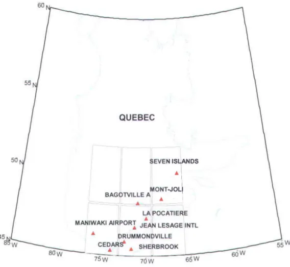
Figure 2 shows the area over southem Quebec, Canada where the studied stations are located. We worked with data sets issued from the following 9 stations located near the Gulf of St. Lawrence: Cedars, Drummondville, Seven Islands, Bagotville, Jean Lesage IntI., Sherbrooke, Maniwaki Airport, La Pocatière and Mont-Joli. For the predictor selection in statistical downscaling, the following data were employed in the CUITent study: 9 series of minimum and maximum temperatures issued from the daily meteorological data from Environment Canada stations, which were homogenized and rehabilitated by Vincent et al. (2002) as predictands (see Table 1 for stations), and a

series of daily normalized predictors from the NCEP-NCAR reanalysis spread over 6 grid-cells of longitude from -67.5° W to -75° W and latitude from 46.39° N to 50.10° N (see Table 2 for the CGCM3 grid-cells). The NCEPINCAR reanalysis data have a grid spacing of 2.5° latitude by 2.5° longitude (DAI MCCG3 predicteurs, 2008).

The predictor data set for the period of 1961 to 1990 was employed. (The data set issued from the NCEPINCAR reanalysis was already standardized for the period of 1961-1990, except for the wind direction.) A total of 25 normalized predictors issued from the NCEPINCAR reanalysis were used in this study aiming to select the most important

(35)

predictors that can fit as weIl as the whole data set using two methods, SWR and lasso; these variables are presented in Table 3. We note that the relative humidity is absent from the predictor list. Due to the high correlation between relative humidity and specific humidity, the relative humidity could be eliminated from the predictor data. However, it is difficult to ensure that these two variables are interchangeable. The predictors are issued from data collected every 6 hours and then standardized on a daily basis using the average (Jl) and the standard deviation (0") for the reference period of 1961-1990 and at the end, the predictors are interpolated linearly on the CGCM3 grid-cells (DAI MCCG3 predicteurs, 2008). The CGCM3 data correspond to the third version of the Canadian Center for Climate Modeling and Analysis (CCCma)-coupled Canadian global climate model. The atmospheric component of the CGCM3 has 31 verticallevels and a horizontal resolution of approximately 3.75° latitude and longitude (approximately 400 km).

5. Results

For aU stations, Tables 4, 5, 6 and 7 show the results of the predictor selection obtained by SWR and lasso for the minimum and maximum temperatures from 1961 to 1990. They present the most important predictors selected that can be used in further downscaling procedures. The predictor selection can be described by a subjective judgment depending on the analyzer. For aU ofthe stations and for both the minimum and maximum temperature, the mean sea level pressure, the geopotential at 850 hPa, the geopotential at 500 hPa, the specific humidity at 850 hPa and the temperature at 2 m can be considered to be the most dominant variables. This seems plausible because these parameters are strongly associated with significant modifications to the temperature characteristics in the boundary layer (see Hessami et al., 2008). The selected predictors

(36)

represent, at sorne level of confidence, almost aIl of the information provided by the whole data set.

Thus, depending on the location of a station relative to the Gulf of St. Lawrence, the selection ofthe most influential predictors can vary slightly. In fact, the selection of sorne meteorological variables at sorne stations depends on the location of the latter relative to the Gulf of St. Lawrence, such as the specific humidity, which represents the amount of water vapor in the air, defined as the ratio of water vapor to dry air at a particular mass. Based on the presence of water in a region, the specific humidity is highly related to temperature variations. In addition to the specific humidity, the temperature at 2 m may be affected by the presence of different air masses influencing temperature variations. F or the 9 stations presented in this work, the mean sea level pressure appears as a common selected predictor for the maximum temperature for both methods. It can be considered to be the most effective predictor, which regroups almost aIl of the predictors' information needed for downscaling; this is somewhat expected because of its great influence on local climate.

Furthermore, the selections by SWR and lasso included the same predictors for the La Pocatière and Maniwaki Airport stations. Otherwise, there is a smaIl difference in the predictor selection for the remaining stations between SWR (Table 4) and lasso (Table 5). Despite this difference, both methods give similar combinations of selected variables, but lasso has the advantage of its automatic aspect of selection. In addition, Lasso did not frequently select predictors 23 and 24 (see Table 3) at the same time as the most effective predictors. Indeed, the 850-hPa specific humidity and the near-surface specific humidity are highly correlated, and one of the specificities of lasso is that it is not affected by

(37)

correlations between predictors, which contributes to its robustness compared to SWR and may improve the selection quality.

According to the results for the minimum temperature, there is a slight difference between the predictors selected by SWR and those selected by lasso. The predictors selected by SWR and lasso are the same for only the Bagotville station: the mean sea level pressure, the geopotential at 850 hPa, the specific humidity at 850 hPa, the near-surface specific humidity and the temperature at 2 m. Otherwise, the predictors selected by SWR randomly differ between stations due to the subjective aspect of the selection process, which depends on the analyzer. Meanwhile, the lasso selection gives more accurate and interpretable models because the most important predictors chosen for aIl of the stations are nearly the same (see Table 6 and Table 7). The most important predictors selected by lasso for the minimum temperature are the mean sea level pressure, the geopotential at 850 hPa, the near-surface specific humidity and the temperature at 2 m, which is consistent with the predictor combinations found for the maximum temperature. The results found for the minimum temperature demonstrate the strength of the lasso technique in dealing with correlations between predictors and in eliminating redundancy. The differences between the lasso and SWR results can be explained by the improved selection achieved by lasso compared to other methods (Grandvalet and Canu, 1999); this improved selection arises from our use of a large data set. Thus, lasso is considered to be a method with enormous potential for extensions and modifications.

To compare the performances of SWR and lasso, a risk function was used (RMSE), incorporating the variance and the square of the estimate bias as weIl as the explained

(38)

variance (R2). Note that lower RMSE values and higher R2 values imply better

performance.

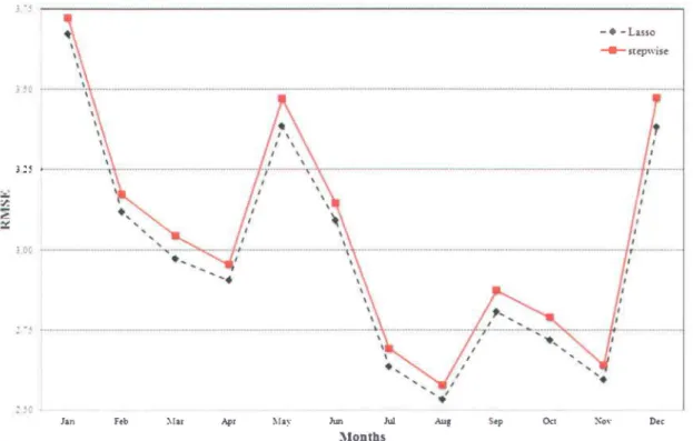
For aU stations over aU months, lasso has lower RMSE and higher R2 values compared to SWR, as shown in Tables 8 and 9 for the maximum temperature and Tables 10 and Il for the minimum temperature. Table 8 summarizes the RMSE results for lasso and SWR for the maximum temperature at aU stations. The RMSE of the maximum temperature varies from 2.01 (Cedars in July) to 4.39 (Bagotville in January) for SWR and from 1.95 (Cedars in July) to 4.25 (Bagotville in January) for lasso. Table 8 indicates that lasso performs better in terms of the RMSE for aU stations and throughout aU months. Figure 3 presents the RMSE for SWR and lasso corresponding to the maximum temperature at the Bagotville station, showing that the error found with SWR is always higher than the one corresponding to lasso. Figure 4 shows the RMSE for lasso and SWR for the maximum temperature at the La Pocatière station. The improved RMSE obtained by lasso is quite clear in this figure, showing that the error achieved by lasso is consistently lower than that obtained with SWR.

Table 9 presents the results of the explained variance (R2) for lasso and SWR for the

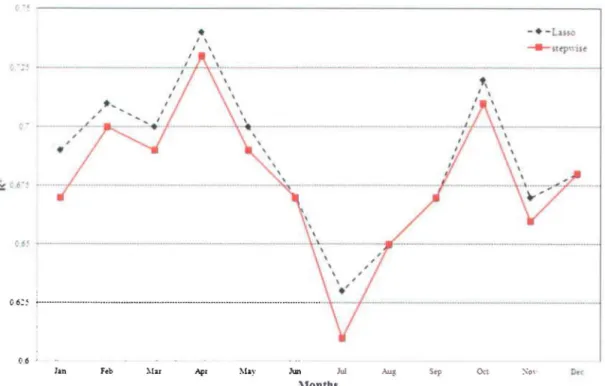
maximum temperature at aU stations. The R 2 value of the maximum temperature varies from 0.39 (Seven Islands in July) to 0.75 (Maniwaki Airport in March) for SWR and from 0.4 (Seven Islands in July) to 0.76 (Maniwaki Airport in March) for lasso. For aU stations and throughout aU months, lasso performs better than stepwise regression in terms of R2• The improvement achieved by lasso is clearly shown in Figure 5, which

presents R2 for both lasso and SWR for the maximum temperature at the Cedars station; the R2 value for lasso is always higher than the one corresponding to SWR. Figure 6

(39)

shows a comparison between lasso and SWR in tenns ofR2 for the maximum temperature at the Jean-Lesage station, emphasizing the improvement obtained by lasso, as weIl as Figure 7, illustrating the R2 values achieved by lasso and SWR for the maximum temperature at the Bagotville station.

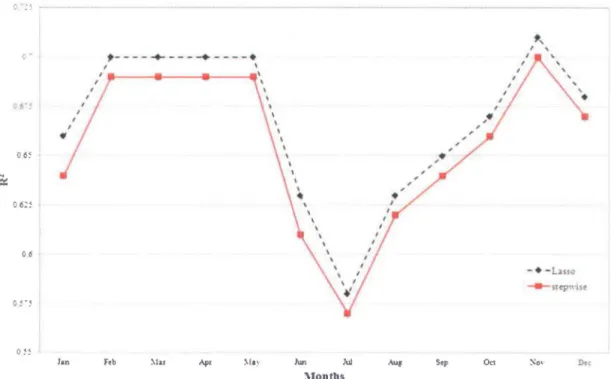
For the minimum temperature, the same trends were observed as for the maximum temperature. Table 10 presents the RMSE results for lasso and SWR for the minimum temperature. The RMSE varies from 1.8 (Seven Islands in July) to 5.67 (Sherbrook in January) for SWR and from 1.79 (Seven Islands in July) to 5.58 (Sherbrook in January) for lasso. Table 10 indicates that lasso perfonns better in tenns of the RMSE for aIl stations and throughout aIl months. In addition, Table 11 presents the R2 results for the minimum temperature for lasso and SWR. The R2 values vary from 0.48 (Seven Islands in July) to 0.72 (Seven Islands in March) for SWR and from 0.49 (Seven Islands in July) to 0.73 (Seven Islands in March) for lasso. The improvement achieved by lasso is c1early shown in Figure 8, which presents R2 for both lasso and SWR for the minimum temperature at the Bagotville station; the R2 values obtained by lasso are higher than those found with SWR. Figure 9 shows the difference between the R2 values found with SWR and those found with lasso for the minimum temperature at the Maniwaki Airport station, emphasizing the improvement in the selection achieved by lasso in tenns of R2.

Thus, lasso perfonned weIl in aIl cases and for aIl stations.

6. Discussion and conclusions

Despite the positive features of the SWR method, the lasso technique perfonned better with the data set employed herein for selecting predictors for downscaling of the

(40)

maXImum and minimum temperature data issued from 9 stations located in eastem Canada near the Gulf of St. Lawrence. Sorne limitations of SWR are overcome by lasso. SWR is based only on correlations and uses only one model throughout treatment of the whole data set. Rence, if the model does not perform well, the selection may not be optimal. Furthermore, with SWR, if a variable has already been eliminated, it cannot be reintroduced to the model, even if it becomes significant. SWR is considered as a highly instable method because the selection can vary strongly if the data are changed even slightly.

The lasso technique combines the positive features of subset selection and ridge regression using stable algorithms as ridge regression and by shrinking sorne coefficients and setting others to zero as the subset selection. Lasso provides easily interpretable models and improves the prediction accuracy.

Moreover, this technique works weIl with large data sets, mainly when p » n (the number of predictors is much higher than the predictand number). There are numerous reports of extensions and modifications of this method, which explains the existence of more than 8 formulations for the lasso technique (see Schmidt, 2005). The usefulness of the lasso method depends on the choice of the tuning parameter as the appropriate choice of t will allow avoiding "over fitting" or "under fitting" of lasso and successful development of the statistical theory.

Two different types of methods were presented in the current study for selecting predictors to compare their performances. Both methods appear to be appropriate to select the smallest number of predictors that can fit the data as well as if we had used the whole data set. Due to its sparseness and its computational advantages, lasso presented a

(41)

better alternative. It is an automated method that is unaffected by collinearity problems, such as correlations between predictors in the regression model, unlike SWR, for which collinearity problems are exacerbated. Thus, lasso achieved lower errors and higher R2 values. SWR behaved weIl in this case, but its results are strongly dependent on the data set used, while lasso can be considered as a more stable method that provides accurate predictions and easily interpretable models.

Both methods obtained good results, but more confidence can be placed in lasso. Many researchers have described the drawbacks of stepwise regression; for example, the R2 values have a high bias, the Fisher and X2 test statistics do not have the claimed distribution, and the standard errors of the parameter estimates are low, causing the confidence intervals around the parameter estimates to be too narrow. Hence, lasso presented a better alternative for predictor selection: it can be implemented in statistical downscaling models (SDSMs) that use SWR for predictor selection, so lasso may improve the accuracy of model outputs. The limitations of lasso include the difficulty encountered in choosing the regularization parameter, which defines the shrinkage rate as weIl as the set of sorne coefficients to zero. Further work may be directed towards implementing this technique in statistical downscaling models and applying lasso to other hydrological variables, such as precipitation.

(42)

Acknowledgments

The authors acknowledge the funding from the National Sciences and Engineering Research Council of Canada (NSERC), the Canada Research Chair Pro gram, and the Ministère du Développement Économique Innovation et Exportation du Québec. The authors acknowledge also the help provided by Dr. Mark Schmidt from l'École Normale Supérieure of Paris and Environment Canada.

(43)

REFERENCES

Breiman, L. 1995. Better subset selection using the non-negative garotte. Technometrics, Vol. 37, No. 4.

Cohen, J and Cohen, P. 1975. Analytic Strategies: Simultaneous, Hierarchical, and Stepwise Regression.pp. 1-18.

Copas, J.B. 1983. Regression, Prediction and Shrinkage. Journal of Royal Statistical Society 45, No 3, pp. 311-354.

DAI MCCG3 predicteurs. 2008: Ensembles de Données de Prédicteurs issus de la Réanalyse du NCEPINCAR et du MCCG3.1 T47. Document disponible via DAI (Données Accès et Integration), version 1.0, Avril 2008, Montréal, QC, Canada, 17 p. Draper, N. R. and Smith, H. 1966. Applied Regression Analysis. Wiley, New York. Efroymson, M.A. 1966. Stepwise Regression-a backward and forward look. Presented at

the Eastern Regional Meetings of the Inst. of Math. Statist., Florham Park, New-Jersey.

Efron. B., Hastie. T., Johnstone. 1. and Tibshirani. R. 2002. Least Angle Regression. Technical report, Standford University.

Fan. J. and Li. R. 2001. Variable Selection via Nonconcave Penalized Likelihood and its Oracle Properties. Journal of the American Statistical Association, Vol. 96, No. 456, Theory and Methods.

(44)

Flom. Peter Land Cassell. David L., NESUG 2007. Stopping stepwise: Why stepwise and similar selection methods are bad, and what you should use. Statistics and Data Analysis.

Frank. 1. E and Friedman. J. H. 1993. A Statistical View of Sorne Chemometrics Regression Tools. Technometrics 35, 109-135.

Goeman, J. 2011. LI and L2 Penalized Regression Models, March 2, 2011.

Grandvalet. 1 and Canu. S. 1999. Outcomes of the equivalence of adaptive ridge with least absolute shrinkage. In NIPS, pages 445-451.

Grandvalet. 1. 1998. Least Absolute Shrinkage is Equivalent to Quadratic Penalization. Hessami. M., Gachon. P., Ouarda. T. B.M.J. and St-Hilaire. A. 2008. Automated

regression-based statistical downscaling tool. Journal Environmental Modeling and Software 23, pp 813-834.

Hoerl. E. Arthur and Kennard. W. Robert. 1970. Ridge Regression: Applications to Nonorthogonal Problems. Technometrics Vo112. No. 1., pp. 69-82.

Hocking, R. R. 1976. A Biometries Invited Paper. The Analysis and Selection of variables in Linear Regression. Biometries, Vol. 32, No. 1., pp. 1-49.

Jennrich, R. 1. and Sampson P.F., 1968. Application of Stepwise Regression to Non-Linear Estimation. Technometrics, Vol. 10, No. 1, pp. 63-72.

Kyung, M., Gill. J., Ghosh, M. and Casella, G. 2010. Penalized Regression, Standard Errors, and Bayesian Lassos. Journal International Society for Bayesian Analysis 5, Number 2, pp. 369-412.

(45)

Lund. Iver. A. 1971. An Application ofStagewise and Stepwise Regression Procedures to a Problem of Estimating Precipitation in California. Journal of Applied Meteorology. Vol. 10, pp. 892-902.

Osborne, M. R., Presnell, B. and Turlach, B. A. 2000a. A new approach to variable selection in least squares problems. IMA Journal of Numerical Analysis 20, pp. 389-404.

Osborne, M. R., Presnell, B. and Turlach, B. A. 2000b. On the LASSO and !ts Dual. Journal ofComputational and Graphical Statistics, Vol. 9, No. 2, pp. 319-337.

Perkins. S., Lacker. K. and Theiler.J., 2003. Grafting: Fast, incremental feature selection by gradient descent in function space. Journal of Machine Learning Research, 3, pp. 1333-1356.

Schmidt, M. December 2005. Least Squares Optimization with LI-Norm Regularization. CS542B Project Report.

Tibshirani, R. 1996. Regression Shrinkage and Selection via the Lasso. Journal of the Royal Statistical Society. Series B (Methodological), Volume 58, Issue 1,267-288. Vincent, L., Zhang, X., Bonsal, B., and Hogg. W., 2002. Homogenization of daily

temperatures over Canada. Journal ofClimate, 15, pp. 1322-1334. Weisberg. S. 2010. Variable Selection and Regularization.

Wenjiang J.Fu. 1998. The Bridge versus the Lasso. Journal of Computational and Graphical Statistics, Vol. 7, No. 3, pp. 397-416.

(46)

APPENDIX 1: NOTATION SECTION

OLS: Ordinary Least Squares method Ale: Akaike Infonnation Criterion BIC: The Bayesian Infonnation Criterion GCM: Global Climate Model

SWR: Stepwise Regression

LASSO: Least Absolute Shrinkage and Selection Operator FS: Forward Selection

BE: Backward Elimination R2: Detennination coefficient

LARS: Least Angle Regression Selection

NCEP: National Center for Environmental Prediction NCAR: National Center for Atmospheric Research MSE: Mean Square Errors

RMSE: Root Mean Square Errors SDSM: Statistical Downscaling Model

(47)

TABLE LIST

Table 1.

Geographical Information of Environment Canada stations

STATION NAME LAT LON ELEV

1 CEDARS 45.30 -74.05 47.00

2 DRUMMONDVILLE 45.88 -72.48 82.00

3 SEVEN ISLANDS 50.22 -66.27 55.00

4 BAGOTVILLE 48.33 -71.00 158.00

5 JEAN LESAGE INTL 46.79 -71.38 74.00

6 SHERBROOKE 45.43 -71.68 240.00

7 MANIW AKI AIRPORT 46.27 -75.99 200.00

8 LA POCATIERE 47.36 -70.03 31.00

9 MONT-JOLI 48.60 -68.22 52.00

Table2.

Longitude, Latitude of the CGCM3 grid cells

Box Number Lon Lat

77X,11Y -75.00 50.10 77X,12Y -75.00 46.39 78X,11Y -71.25 50.10 78X,12Y -71.25 46.39 79X,11Y -67.50 50.10 79X,12Y -67.50 46.39

(48)

Table3.

NCEPINCAR predictor variables on CGCM3 grid

No. Predictor No. Predictor

1 Mean sea level pressure 14 500hPa divergence 2 Surface airflow strength 15 850hPa airflow strength 3 Surface zonal velo city 16 850hPa zonal velocity 4 Surface meridional velo city 17 850hPa meridional velo city 5 Surface vorticity 18 850hPa vorticity

6 Surface wind direction 19 850hPa geopotential 7 Surface divergence 20 850hPa wind direction 8 500hPa airflow strength 21 850hPa divergence 9 500hPa zonal velocity 22 500hPa specific Humidity 10 500hPa meridional velocity 23 850hPa specific Humidity

11 500hPa vorticity 24 Near surface specific Humidity 12 500hPa geopotential 25 Temperature at 2m

13 500hPa wind direction

Table 4.

Results of the most important predictors selected for the maximum temperature by SWR

Station Predictors

Cedars 1 5 19 23 24

Drummondville 1 19 23 24 25

Seven Islands 1 19 23 24 25

Bagotville 1 19 23 24 25

Jean Lesage IntI 1 19 23 24 25

Sherbrooke 1 19 23 24 25

Maniwaki Airport 1 19 23 24 25