arXiv:1707.02064v1 [astro-ph.SR] 7 Jul 2017
Astronomy & Astrophysicsmanuscript no. hd166734x c ESO 2017
July 10, 2017
An X-ray view of HD 166734, a massive supergiant system
⋆
Ya¨el Naz´e
⋆⋆, Eric Gosset
⋆⋆⋆, Laurent Mahy
†, and Elliot Ross Parkin
Groupe d’Astrophysique des Hautes Energies, STAR, Universit´e de Li`ege, Quartier Agora (B5c, Institut d’Astrophysique et de G´eophysique), All´ee du 6 Aoˆut 19c, B-4000 Sart Tilman, Li`ege, Belgium
e-mail: [email protected] Preprint online version: July 10, 2017
ABSTRACT
The X-ray emission of the O+O binary HD 166734 was monitored using Swift and XMM-Newton observatories, leading to the discovery of phase-locked variations. The presence of an f line in the He-like triplets further supports a wind-wind collision as the main source of the X-rays in HD 166734. While temperature and absorption do not vary significantly along the orbit, the X-ray emission strength varies by one order of magnitude, with a long minimum state (∆(φ) ∼ 0.1) occurring after a steep decrease. The flux at minimum is compatible with the intrinsic emission of the O-stars in the system, suggesting a possible disappearance of colliding wind emission. While this minimum cannot be explained by eclipse or occultation effects, a shock collapse may occur at periastron in view of the wind properties. Afterwards, the recovery is long, with an X-ray flux proportional to the separation d (in hard band) or to d2(in soft band). This is incompatible with an adiabatic nature for the collision (which would instead lead to FX∝1/d), but could be
reconciled with a radiative character of the collision, though predicted temperatures are lower and more variable than in observations. An increase in flux around φ ∼ 0.65 and the global asymmetry of the light curve remain unexplained, however.
Key words.stars: early-type – stars: winds – X-rays: stars – stars: individual: HD 166734
1. Introduction
Stellar winds are a key ingredient in the lives of massive stars, but their exact properties are still a subject of debate. To gain further insight into these winds, there are several observational opportunities, such as analyses of P Cygni profiles in the UV spectra of single stars or of colliding wind emission in binaries. Indeed, when two massive stars form a gravitationally bound pair, their winds collide, and the characteristics of this interac-tion depends on the relative strengths of the winds.
These collisions produce signatures over a wide range of wavelengths; in particular, for some massive binaries, the post-shock temperature is so high that X-rays are emitted. The main observational characteristics of such an emission is its variabil-ity due to a variety of factors (for a review, see Rauw & Naz´e 2016): the absorption towards the collision zone changes as it is seen through different wind densities over an orbital period, the collision strength depends on the stellar separation in eccen-tric binaries, and occultation of the collision zone by the stellar bodies may occur, as well as hysteresis effects. The observed variations thus depend on stellar and orbital parameters, but also on the orientation of the system with respect to Earth and on the details of plasma physics.
In this context, it would be extremely interesting to com-pare systems with similar orbits and orientations but different wind momentum ratios as they would provide a kind of “con-trolled experiment” to test our understanding of such wind-wind ⋆ Based on observations collected with Swift and the ESA science
mission XMM-Newton, an ESA Science Mission with instruments and contributions directly funded by ESA Member States and the USA (NASA).
⋆⋆ F.R.S.-FNRS Research Associate. ⋆⋆⋆ F.R.S.-FNRS Senior Research Associate.
† F.R.S.-FNRS Postdoctoral Researcher.
collisions. Recently, we have analysed the case of the eccen-tric binary WR21a (Gosset & Naz´e, 2016). Its period is ∼32 d and its eccentricity e ∼ 0.7, which are close to those of an-other massive binary: HD 166734. However, these binaries have very different wind momentum ratios: ˙M1v∞,1/ ˙M2v∞,2is about 7
for WR21a (Gosset & Naz´e, 2016), but only ∼3 for HD 166734 (Mahy et al., 2017, hereafter Paper I). Since HD 166734 has never been studied at X-ray wavelengths, we have undertaken a specific X-ray monitoring of this system, with the hope of con-straining the properties of its wind-wind collision.
This paper investigates the X-ray emission of HD 166734 as observed by Swift and XMM-Newton. Section 2 provides some information on the target, Sect. 3 presents the data and their duction, Sect. 4 explains the analysis, Sect. 5 discusses the re-sults, and Sect. 6 summarizes and concludes.
2. The target
The binarity of HD 166734 was first reported by Wolff (1963) but the monitoring of Conti et al. (1980) provided the first or-bital solution of the system. These authors found the period to be 34.54 d and the masses of the stars to be similar despite different spectral types (O7.5If+O9I). In view of their masses, Conti et al. (1980) also proposed that eclipses occur in HD 166734, and eclipses were indeed reported for the system by Otero & Wils (2005), although there is only one per orbit. No additional visual companion was detected around the central binary (Mason et al., 2009; Sana et al., 2014).
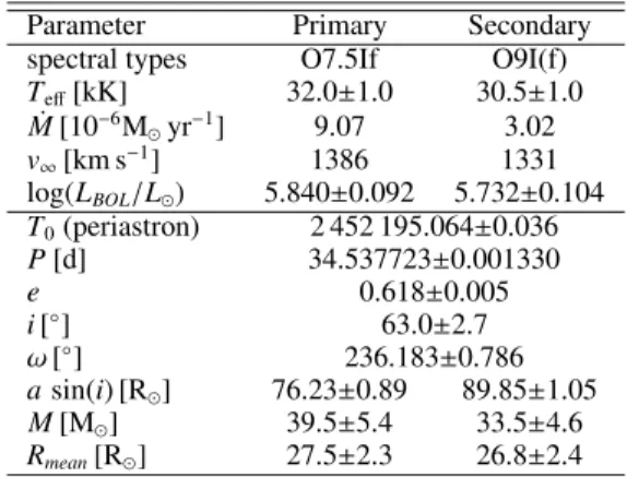
Recently, Paper I revisited the system using dedicated pho-tometric and spectroscopic monitorings. The orbital parameters of HD 166734 were then refined and the stellar characteristics of each of its components determined, thanks to the derivation of the individual spectra using disentangling methods and the spectral fitting made with atmosphere models. Table 1
summa-Table 1.Stellar and orbital parameters derived in Paper I.
Parameter Primary Secondary
spectral types O7.5If O9I(f)
Teff[kK] 32.0±1.0 30.5±1.0 ˙ M[10−6M⊙yr−1] 9.07 3.02 v∞[km s−1] 1386 1331 log(LBOL/L⊙) 5.840±0.092 5.732±0.104 T0(periastron) 2 452 195.064±0.036 P[d] 34.537723±0.001330 e 0.618±0.005 i[◦] 63.0±2.7 ω[◦] 236.183±0.786 asin(i) [R⊙] 76.23±0.89 89.85±1.05 M[M⊙] 39.5±5.4 33.5±4.6 Rmean[R⊙] 27.5±2.3 26.8±2.4
rizes the new parameters of the system, which we will use in this follow-up paper.
3. Observations and data reduction
3.1.XMM-Newton
The first XMM-Newton observation of HD 166734, available in the archives, was taken in March 2008 (Principal Investigator Valencic). It shows a bright source, with a count rate compatible with ROSAT values. However, in view of the variations seen in the Swift data (see below), we requested in March 2016 a sec-ond short exposure to sample the phase of minimum flux. It was granted under Director Discretionary Time. Both datasets were reduced with SAS (Science Analysis Software) v15.0.0 using calibration files available in Spring 2016 and following the rec-ommendations of the XMM-Newton team1.
The EPIC (European Photon Imaging Camera) observations, taken in the full-frame mode and with the medium filter (to reject optical/UV light), were filtered to keep only the best-quality data (pattern of 0–12 for MOS and 0–4 for pn). Background flares were detected in the first observation, and they were cut before engaging in further analyses. A source detection was performed on each EPIC dataset using the task edetect chain on the 0.5–1.5 (soft) and 1.5–10.0 (hard) energy bands and for a log-likelihood of 10. This task searches for sources using a sliding box and de-termines the final source parameters from point spread function (PSF) fitting; the final count rates correspond to equivalent on-axis, full PSF count rates (Table 2).
We then extracted EPIC spectra of HD 166734 using the task especget in circular regions of 36′′radius (to avoid nearby
sources) centred on the best-fit positions found for each ob-servation. For the background, a circular region of 40′′ radius
was chosen in a region devoid of sources and as close as pos-sible to the target; its relative position with respect to the tar-get is the same for both observations. Dedicated ARF (Ancillary Response File) and RMF (Redistribution Matrix File) response matrices, which are used to calibrate the flux and energy axes, re-spectively, were also calculated by this task. EPIC spectra were grouped with specgroup to obtain an oversampling factor of five and to ensure that a minimum signal-to-noise ratio of 3 (i.e. a minimum of 10 counts) was reached in each spectral bin of the background-corrected spectra.
EPIC light curves of HD 166734 were extracted for time bins of 100 s, 500 s, and 1 ks, in the same regions as the spectra, and
1 SAS threads, see
http://xmm.esac.esa.int/sas/current/documentation/threads/
in the same energy bands (plus the total one, 0.5–10. keV band) as the source detection. They were further processed by the task
epiclccorr, which corrects for loss of photons due to vignetting,
off-axis angle, or other problems such as bad pixels. In addi-tion, to avoid very large errors and bad estimates of the count rates, we discarded bins displaying effective exposure time lower than 50% of the time bin length. Our previous experience with XMM-Newton has shown us that including such bins degrades the results. As the background is much fainter than the source, in fact too faint to provide a meaningful analysis, three sets of light curves were produced and analysed individually: the raw source+background light curves, the background-corrected light curves of the source, and the light curves of the sole background region. The results found for the raw and background-corrected light curves of the source are indistinguishable.
The EPIC count rates of HD 166734 in the first observation (1.6 cts s−1for pn and 0.5 cts s−1for MOS) are close to the
pile-up limits (∼2 and ∼0.5 cts s−1for pn and MOS, respectively). We
therefore checked the presence of pile-up using the task epatplot, which did not show any clear evidence of pile-up. Furthermore, we extracted spectra of HD 166734 in an annulus centred on the source and considering only single events (pattern=0). Again, no evidence for pile-up is detected as spectral fitting provide re-sults in agreement with those found using spectra derived in the usual way.
Only RGS (Reflection Grating Spectrometer) spectra of the first observation have enough counts for a scientific analysis. No flare filtering was applied, however, as the background light curve showed an elevated level throughout the exposure rather than localized flares. The source and background spectra were extracted in the default regions as HD 166734 has no neighbour of similar X-ray brightness. Dedicated response files were cal-culated for both orders and both RGS, and were subsequently attached to the source spectra for analysis.
3.2. Swift
At our request, HD 166734 was observed 17 times by Swift be-tween February and April 2016 (Table 2). These data were re-trieved from the HEASARC (High-Energy Astrophysics Science Archive Research Center). Since the target is quite bright (V=8.42), UVOT (Ultraviolet/Optical Telescope) cannot be used and XRT (X-ray Telescope) data, which were taken in PC (Photon Counting) mode, could suffer from optical loading, re-quiring a check. Using the dedicated web tool2 for the
appro-priate properties of our target (Teff=30.5–32 kK, BC between –
2.8 and –3.0), we found that spurious events from optical load-ing would at most lead to 10−5cts s−1. This is well below the
detected values for the target, hence the optical loading can be considered negligible.
XRT data taken in PC mode were processed locally us-ing the XRT pipeline of HEASOFT (High-Energy Astrophysics Software) v6.18 with calibrations available in Spring 2016. Corrected count rates in the same energy bands as XMM-Newton were obtained for each observation from the UK online tool3
(Table 2). It also provided the best-fit position for the full dataset, which is similar to Simbad’s value. The Simbad position was thus used to extract the source spectra within Xselect in a circular region of 50′′radius (as recommended). They were binned using
grpphain a similar manner to that used for the XMM-Newton
spectra. Following the recommendations of the Swift team, the 2 http://www.swift.ac.uk/analysis/xrt/optical tool.php
Table 2.Journal of the X-ray observations: X for XMM-Newton observations and S for Swift exposures. HJD correspond to dates at mid-exposure, and the corresponding phases were calculated using the ephemeris of Paper I; exposure times correspond to on-axis values (for pn if XMM-Newton). The XMM-Newton count rates correspond to the sum of MOS1, MOS2, and pn values. We note that the Swift XID notation follows the ObsID naming scheme (there is thus no S-1 as 00034304001 has zero seconds of useful time).
XID ObsID (exp. time) HJD φ Count Rates (cts s−1)
0.5–1.5 keV 1.5–10.0 keV X-1 0500030101 (47.6 ks) 2454531.604 0.65 1.707±0.007 0.927± 0.005 X-2 0790180601 (8.0 ks) 2457480.796 0.04 0.131± 0.005 0.054± 0.004 S-2 00034304002 (0.7 ks) 2457428.242 0.52 0.0743± 0.0145 0.0395± 0.0100 S-3 00034304003 (3.2 ks) 2457429.903 0.57 0.0592± 0.0050 0.0403± 0.0040 S-4 00034304004 (3.4 ks) 2457433.340 0.67 0.0727± 0.0052 0.0508± 0.0043 S-5 00034304005 (2.3 ks) 2457436.002 0.75 0.0674± 0.0059 0.0467± 0.0049 S-6 00034304006 (1.0 ks) 2457438.692 0.82 0.0863± 0.0126 0.0462± 0.0085 S-7 00034304007 (3.7 ks) 2457441.646 0.91 0.0334± 0.0034 0.0251± 0.0030 S-8 00034304008 (2.8 ks) 2457444.605 0.99 0.0068± 0.0018 0.0040± 0.0014 S-9 00034304009 (3.8 ks) 2457447.656 0.08 0.0070± 0.0015 0.0035± 0.0011 S-10 00034304010 (2.8 ks) 2457453.179 0.24 0.0249± 0.0033 0.0228± 0.0031 S-11 00034304011 (2.0 ks) 2457455.908 0.32 0.0360± 0.0056 0.0331± 0.0052 S-12 00034304012 (1.4 ks) 2457456.626 0.34 0.0484± 0.0064 0.0429± 0.0061 S-13 00034304013 (1.4 ks) 2457476.611 0.92 0.0266± 0.0050 0.0293± 0.0054 S-14 00034304014 (1.9 ks) 2457480.297 0.03 0.0066± 0.0020 0.0036± 0.0016 S-15 00034304015 (1.5 ks) 2457484.685 0.16 0.0136± 0.0032 0.0158± 0.0035 S-16 00034304016 (0.8 ks) 2457486.085 0.20 0.0254± 0.0066 0.0164± 0.0053 S-17 00034304017 (0.3 ks) 2457486.887 0.22 0.0176± 0.0089 0.0087± 0.0063 S-18 00034304018 (3.8 ks) 2457494.506 0.44 0.0518± 0.0040 0.0349± 0.0033
largest possible background region was chosen, i.e. an annulus of outer radius 100′′. The most recent RMF matrix from the
cali-bration database was used while specific ARF response matrices were calculated for each dataset using xrtmkarf, considering the associated exposure map.
Because of the small number of counts and the excellent re-peatability with phase of the light curve (see next section), we combined some Swift spectra taken at similar phases using the ftoolsaddpha and addarf: 8, 9, and 14 (φ ∼ 0.03); S-10, S-15, and S-16 (φ ∼ 0.20); S-11 and S-12 (φ ∼ 0.33); S-7 and S-13 (φ ∼ 0.91). The weights for ARF combinations were in proportion to the number of counts in the individual spectra. In contrast, the spectra of datasets S-2, S-6, and S-17 had too few counts to be useful, so we discarded them from the spectral analyses.
4. Results
4.1. Light curves
At first glance, the data directly show large variations in the X-ray brightness of HD 166734 (see Table 2 and left panel of Fig. 1). The amplitude of the variations is very large: the ratio be-tween the extreme count rates exceeds one order of magnitude. To understand the nature of such changes, it is important to note that the Swift data were taken during two consecutive orbits of the system. Folding them with the orbital period yields a remark-able agreement, demonstrating the repeatability of these changes (Fig. 1). In particular, it is worth noting the quasi-identity be-tween two data points taken in different orbits (S-7 and S-13): as both belong to the steep descending branch, any phase shift would have been readily detected if the wrong timescale had been used. Moreover, the two XMM-Newton datasets, taken 8 years apart (corresponding to 85 orbits), also agree well with the
Swiftlight curve. Clearly, the variations of the X-ray emission
of HD 166734 are phase-locked in nature. Fortunately, the Swift data cover the full 34.54 d orbit in a homogeneous manner.
The light curve of HD 166734 shows a flat minimum lasting ∆(φ)=0.1 around periastron (from φ=0.99 to 0.08). This mini-mum is preceded by a steep, order-of-magnitude decrease, be-ginning after φ ∼ 0.8. It is followed by a shallower increase up to φ ∼ 0.5 and a quasi-flattening afterwards. The same behaviour is detected in both the soft and hard bands, so that there are no drastic changes in hardness (see right panel of Fig. 1): in the more sensitive XMM-Newton data, the ratio between hard and soft count rates only changes from 0.41±0.03 (at minimum flux) to 0.543±0.004, i.e. there is a significant (4σ) but limited soft-ening at minimum flux; in the Swift data, there is also a slight increase in hardness near φ=0.2–0.3, but it remains within 2σ of the other values.
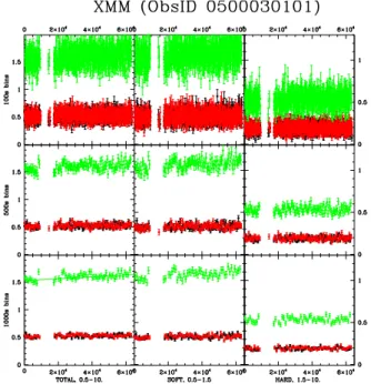
The first XMM-Newton observation covers half a day. We have thus analysed the intra-pointing variability of that dataset (Fig. 2) using χ2 tests for three different null hypotheses
(con-stancy, linear variation, quadratic variation). The improvement in the χ2when increasing the number of parameters in the model
(e.g. linear trend vs constancy) was also determined by means of Snedecor F tests (nested models; see Sect. 12.2.5 in Lindgren, 1976). While all light curves are formally compatible with a con-stant level (even for significance levels of 1%), we found that the soft and total pn light curves were significantly better fitted by a linear trend. This trend is also detected in soft and total MOS light curves, but at the 5% significance level only (which can be explained by the lower sensitivity of these cameras). The slope is 2.5×10⁻⁶cts s−2for the sum of all EPIC data. When
overplot-ted on the global light curve (left panel of Fig. 1), this increasing trend corresponds to the increase observed between the S-3 and S-4 datasets. It is, however, steeper than the overall shallow in-crease seen for φ=0.5–0.8.
4.2. Global spectral fitting
We fitted the spectra under Xspec v12.9.0i, considering refer-ence solar abundances from Asplund et al. (2009). As X-ray
0 0.2 0.4 0.6 0.8 1 0 1 2 3 (XMM-EPIC,Swift*21.6) 0.5 1 1.5 0 0.2 0.4 0.6 0.8 1 -200 -100 0 100 200 Primary in front
Count Rates (XMM-EPIC + Swift*21.6)
0 0.5 1 1.5 2 0 0.5 1 0 0.2 0.4 0.6 0.8 1 0 0.5 1
Fig. 1.Variation in the count rates and hardness ratio with orbital phase for XMM-Newton (black dots) and Swift data (empty green squares for S-2 to 12 from Feb-March 2016, blue triangles for S-13 to 18 from April 2016; see Table 2). For all energy bands, Swift count rates and their errors were multiplied by 21.6 to clarify the trends (no further treatment was made for adjustment). In the top left panel, the straight red line represents the trend detected in the intra-pointing light curve of X-1. To help the comparison with physical parameters, the bottom left panels provide the orbital separation (in units of the semi-major axis a) as well as a position angle defined as zero when the O7.5I star (primary) is in front and 180◦when the O9I star (secondary) is in front. The vertical lines
in the top left panel indicate the phases of the quadratures, conjunctions, and optical eclipse start/end. All data are phased according to the ephemeris of Paper I.
Fig. 2.Intra-pointing light curves of the first XMM-Newton ob-servations (pn in green, MOS1 in black, MOS2 in red). The top, middle, and bottom panels show the light curves with 100 s, 500 s, and 1000 s time bins, respectively, while the left, central, and right panels display the total, soft, and hard light curves. The ordinates in cts s−1 are given on the left side for the total light
curves, but on the right side for the soft and hard light curves. In the bottom left panel, the best-fit linear trend is superimposed onto the pn data.
lines are clearly detected on both low- and high-resolution spec-tra, absorbed optically thin thermal emission models (of the type
wabs × phabs ×Papec) were considered. The first absorption
component represents the interstellar contribution. It was fixed to 8.1 × 1021cm−2, calculated using the reddening of the target
(E(B − V) = 1.33, from B − V=1.07 and (B − V)0= −0.26), and
the conversion factor from Gudennavar et al. (2012).
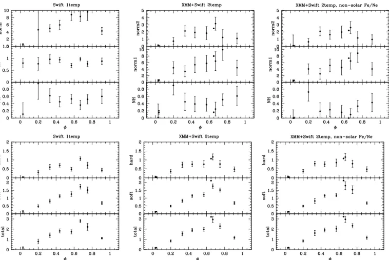
The Swift spectra have a low number of counts, they can thus be fitted with a single thermal component (Table 3, Fig. 3). The normalization factors and the fluxes follow the light curve based on count rates (see previous subsection and Fig. 1). The derived temperature appears constant at 0.85 keV on average. The ab-sorption appears slightly lower at minimum flux, slightly higher just afterwards, and very stable at other phases; however, these changes are at the 1–2σ level only. Fits forcing the absorption to remain at a constant value (the mean of the values obtained earlier) results in a marked (though not large) increase in the χ2
for the spectra taken at φ ∼ 0.15.
All XMM-Newton spectra were fitted simultaneously, i.e. all EPIC+RGS for X-1 and all EPIC for X-2. These spectra could not be fitted with a single temperature, but the sum of two ther-mal components provides an excellent fit except in the 1.–2. keV range for the EPIC spectra of X-1. For this dataset, using individ-ual absorptions for each thermal component does not improve the quality of the fit but the χ2 can be improved by changing
some abundances (not the global metallicity). Since the RGS spectra clearly show Ne, Mg, and Fe lines (see Sect. 4.3) and since these elements are responsible for lines in the 1.–2. keV range, we only allow the abundances of these elements to vary4. 4 Paper I found departures from solar abundances for HeCNO, but
Fig. 3.Results of the spectral fits for the three types of fits performed (Table 3). The three panels on the top line provide the variations with phase of the spectral parameters (norm in units 10−3cm−5, kT in keV, and N
Hin units 1022cm−2) while the three panels on the
bottom line yield observed fluxes in units 10−12erg cm−2s−1. The panel pairs in the left, middle, and right columns correspond to
results from single temperature fits, two-temperature fits with solar abundances, and two-temperature fits with non-solar abundances, respectively.
In all the trials we performed, the Fe abundance became subso-lar and the Mg abundance stayed close to 1. The Ne abundance has a mixed behaviour. It appears slightly subsolar when fitted on RGS data alone, but is clearly oversolar when fitted on EPIC or EPIC+RGS spectra. Physically, this result is puzzling, but we know from experience that abundances found in EPIC spectra are not to be trusted blindly and that they have limited informa-tive value. We therefore performed two sets of fits, one with solar abundances and a second set with Ne and Fe abundances fixed to the best-fit values found by fitting the full first XMM-Newton dataset (i.e. both EPIC and RGS data). Since we detect no clear change in temperature between the two XMM-Newton datasets, and since there was no significant temperature variation in the
Swiftdata, the temperatures were also fixed to the best-fit
val-ues found for the first XMM-Newton dataset. Results for both cases (solar and non-solar abundances) are provided in Table 3 and Fig. 3: the trends are similar in both cases. Furthermore, they agree well with the results from simple fits to the Swift spectra. It should be further noted that no significant change in absorption is detected between the two XMM-Newton datasets and that the average temperature varies by only 20% between the two
XMM-data cannot be used to constrain these abundances for the hot plasma, hence we kept these elements to solar values. However, as demonstrated below for Ne and Fe, changing abundances would not affect our con-clusions.
Newtondatasets (confirming the hardness ratio results). Finally,
the hard flux appears stable in the φ = 0.3 − 0.8 interval except for a peak at φ ∼ 0.65 which corresponds well to the increase detected in the first XMM-Newton dataset.
4.3. X-ray lines
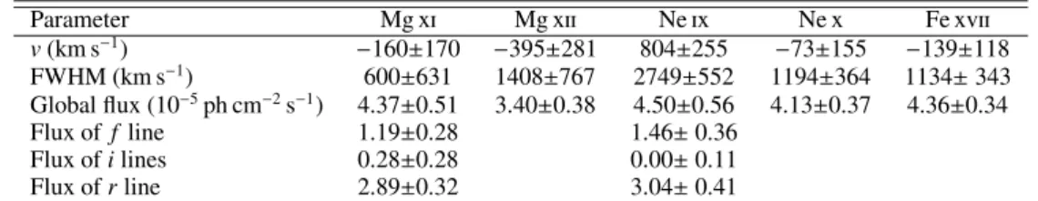
Because of the strong interstellar absorption in front of HD 166734 and the low sensitivity of RGS at high energies, the combined RGS spectrum (Fig. 4) only shows a few lines: the Lyman-α and He-like ratios of Ne and Mg, and some Fe xvii lines near 15Å and 17Å. Line fitting of the ungrouped raw (i.e. without background subtraction) spectra were performed using the Cash statistics and following two methods.
First, we used a flat power law (to represent the background level) combined with a sum of Gaussians. For Lyman-α and the Fe doublet at 15Å, two Gaussians were used with their respective amplitudes fixed to the theoretical value5. For He-like “triplets”
(with its f ir components), four Gaussians were used and only the relative amplitude of the central two intercombination lines was fixed to the theoretical value. In both cases, the widths and shifts of all Gaussians were assumed to be the same. Table 4 lists the results of these fits. The most reliable results come from the
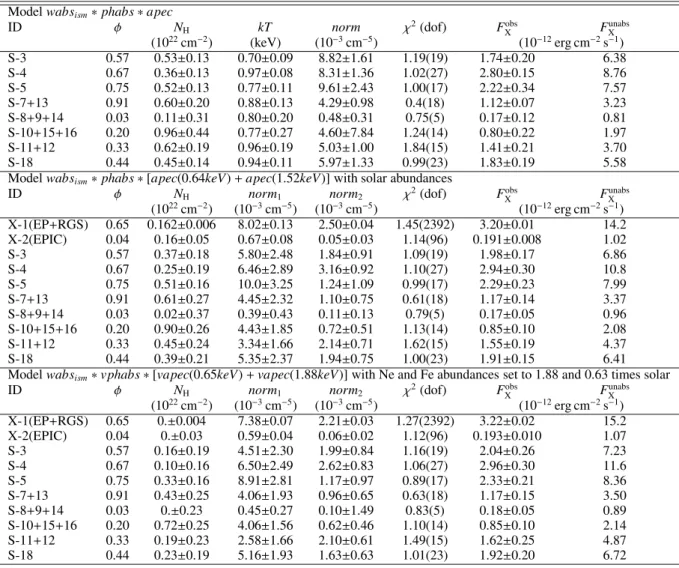
Table 3.Results of the global spectral fits.
Model wabsism∗phabs ∗ apec
ID φ NH kT norm χ2(dof) FXobs FXunabs
(1022cm−2) (keV) (10−3cm−5) (10−12erg cm−2s−1) S-3 0.57 0.53±0.13 0.70±0.09 8.82±1.61 1.19(19) 1.74±0.20 6.38 S-4 0.67 0.36±0.13 0.97±0.08 8.31±1.36 1.02(27) 2.80±0.15 8.76 S-5 0.75 0.52±0.13 0.77±0.11 9.61±2.43 1.00(17) 2.22±0.34 7.57 S-7+13 0.91 0.60±0.20 0.88±0.13 4.29±0.98 0.4(18) 1.12±0.07 3.23 S-8+9+14 0.03 0.11±0.31 0.80±0.20 0.48±0.31 0.75(5) 0.17±0.12 0.81 S-10+15+16 0.20 0.96±0.44 0.77±0.27 4.60±7.84 1.24(14) 0.80±0.22 1.97 S-11+12 0.33 0.62±0.19 0.96±0.19 5.03±1.00 1.84(15) 1.41±0.21 3.70 S-18 0.44 0.45±0.14 0.94±0.11 5.97±1.33 0.99(23) 1.83±0.19 5.58
Model wabsism∗phabs ∗[apec(0.64keV) + apec(1.52keV)] with solar abundances
ID φ NH norm1 norm2 χ2(dof) FXobs FunabsX
(1022cm−2) (10−3cm−5) (10−3cm−5) (10−12erg cm−2s−1) X-1(EP+RGS) 0.65 0.162±0.006 8.02±0.13 2.50±0.04 1.45(2392) 3.20±0.01 14.2 X-2(EPIC) 0.04 0.16±0.05 0.67±0.08 0.05±0.03 1.14(96) 0.191±0.008 1.02 S-3 0.57 0.37±0.18 5.80±2.48 1.84±0.91 1.09(19) 1.98±0.17 6.86 S-4 0.67 0.25±0.19 6.46±2.89 3.16±0.92 1.10(27) 2.94±0.30 10.8 S-5 0.75 0.51±0.16 10.0±3.25 1.24±1.09 0.99(17) 2.29±0.23 7.99 S-7+13 0.91 0.61±0.27 4.45±2.32 1.10±0.75 0.61(18) 1.17±0.14 3.37 S-8+9+14 0.03 0.02±0.37 0.39±0.43 0.11±0.13 0.79(5) 0.17±0.05 0.96 S-10+15+16 0.20 0.90±0.26 4.43±1.85 0.72±0.51 1.13(14) 0.85±0.10 2.08 S-11+12 0.33 0.45±0.24 3.34±1.66 2.14±0.71 1.62(15) 1.55±0.19 4.37 S-18 0.44 0.39±0.21 5.35±2.37 1.94±0.75 1.00(23) 1.91±0.15 6.41
Model wabsism∗vphabs ∗[vapec(0.65keV) + vapec(1.88keV)] with Ne and Fe abundances set to 1.88 and 0.63 times solar
ID φ NH norm1 norm2 χ2(dof) FXobs FXunabs
(1022cm−2) (10−3cm−5) (10−3cm−5) (10−12erg cm−2s−1) X-1(EP+RGS) 0.65 0.±0.004 7.38±0.07 2.21±0.03 1.27(2392) 3.22±0.02 15.2 X-2(EPIC) 0.04 0.±0.03 0.59±0.04 0.06±0.02 1.12(96) 0.193±0.010 1.07 S-3 0.57 0.16±0.19 4.51±2.30 1.99±0.84 1.16(19) 2.04±0.26 7.23 S-4 0.67 0.10±0.16 6.50±2.49 2.62±0.83 1.06(27) 2.96±0.30 11.6 S-5 0.75 0.33±0.16 8.91±2.81 1.17±0.97 0.89(17) 2.33±0.21 8.36 S-7+13 0.91 0.43±0.25 4.06±1.93 0.96±0.65 0.63(18) 1.17±0.15 3.50 S-8+9+14 0.03 0.±0.23 0.45±0.27 0.10±1.49 0.83(5) 0.18±0.05 0.89 S-10+15+16 0.20 0.72±0.25 4.06±1.56 0.62±0.46 1.10(14) 0.85±0.10 2.14 S-11+12 0.33 0.19±0.23 2.58±1.66 2.10±0.61 1.49(15) 1.62±0.25 4.87 S-18 0.44 0.23±0.19 5.16±1.93 1.63±0.63 1.01(23) 1.92±0.20 6.72
Notes.The first part of the table presents fits with a single thermal component (Swift data only), while the second and third parts list the fitting results for two thermal components of fixed temperatures for solar abundances and for non-solar Ne and Fe abundances. Unabsorbed fluxes are only corrected for the interstellar column (8.1 × 1021cm−2). Errors (found using the “error” command for the spectral parameters and the “flux
err” command for the fluxes) correspond to 1σ; whenever errors were asymmetric, the highest value is provided here. Fluxes are expressed in the 0.5–10.0 keV band.
doublets as they are the strongest and most isolated lines: no sig-nificant shift is detected and the line FWHMs are similar to the terminal wind velocity (∼1350 km s−1, see Table 1), as is usual
for O-stars (Waldron & Cassinelli, 2007). The noisier triplets agree with these results, within 2–3σ. These triplets can be used for two additional derivations. The temperature can be estimated from the G = ( f + i)/r ratios, and from the ratios between the Lyman-α intensities and the combined ( f + i + r) He-like triplet line strengths; however, the latter ratios must be corrected for the effect of (interstellar) absorption, as the Lyman-α and He-like triplet lines are at different wavelengths, hence they suf-fer from difsuf-ferent absorption effects. Following the method out-lined in Naz´e et al. (2012a), but considering the latest version of ATOMDB, we derive log(T )=6.9–7.0 for Mg and log(T )=6.6– 7.0 for Ne. These temperatures agree well with those found in spectral fits (Table 3 - 0.65, 0.85, and 1.88 keV correspond-ing to log(T )=6.9, 7.0, and 7.3, respectively). Furthermore, the
f /i line ratio can be used to constrain where the X-ray
emit-ting plasma lies with respect to the star (Porquet et al., 2001; Leutenegger et al., 2006). In our case, however, we have the problem that only an upper limit on the i line strength is
avail-able, so that only the lower limits of the ratios can be found:
f /i > 1.6 for Mg and > 10 for Ne, considering the upper limit
of the i line strength and the best-fit strength minus 1σ for the
f line. The former value agrees well with the expected
theoret-ical ratio without any depopulation of the upper level of the f line (1.–2. for temperatures in the log(T )=6.9–7.3 range). The latter value is too high with respect to the theoretical ratio, but considering a 3σ uncertainty on the strength of the lines rec-onciles the observed value with the expected ones. Despite the high uncertainty, it seems clear that the f line exists, and with a strength suggesting no depopulation by UV photons: the X-ray emitting plasma is thus located far from the stellar surfaces. This agrees well with an origin in a colliding-wind shock; in fact, de-tecting an f line but no (or faint) i line is usually considered as evidence for the presence of such collisions (e.g. Schild et al., 2004; Pollock et al., 2005; Sugawara et al., 2008; Zhekov et al., 2014).
Second, we used the windprofile package available for Xspec6. It models the line profiles expected for shocks
10 15 20 0 0.0002 0.0004 0.0006 Fe XVII 8.5 9 9.5 0 0.0001 0.0002 0.0003 0.0004 0.0005 Mg r i f 12 12.5 13 13.5 14 Ne r i f 15 Fe XVII
Fig. 4. The combined RGS spectrum for dataset X-1. The top panel shows a close-up on the strongest lines.
tributed throughout the wind (Leutenegger et al., 2006, and ref-erences therein). In addition to the line strength, its two most important parameters are τ∗, the characteristic continuum
opti-cal depth of the wind as defined in Owocki & Cohen (2001), and
R0, the radius at which the X-ray emission begins. For He-like
triplets, the relative strengths of the components are also derived. While the overall line strengths and the G ratios of the He-like triplets agree well with those found by the first method, the other parameters are ill-constrained; we are not able to draw more pre-cise conclusions from these models than we do from our simple fits.
5. Discussion
In this section, we try to interpret, one at a time, the observational results presented above.
First, HD 166734 presents an exceptionally deep (one or-der of magnitude) and long (∆(φ) ∼ 0.1) X-ray minimum. For comparison, WR21a shows no flat bottom and the X-ray flux changes only by a factor of 4 between apastron and pe-riastron (Gosset & Naz´e, 2016). In WR140, the flat minimum lasts only 0.01 in phase and a flux ratio of two is observed between apastron and periastron (Corcoran et al., 2011). Only ηCar appears to have a very low minimum, with a one or-der of magnitude decrease in the hard flux (Hamaguchi et al., 2014), but it lasts only 0.01–0.03 in phase (Corcoran et al., 2010). HD 166734 thus appears to be an extreme case and the cause for this long and deep minimum needs to be investigated. The question arises of whether the X-ray emission associated with the wind collision completely disappears at periastron in HD 166734. When the emission is bright, the high-resolution XMM-Newton spectra clearly indicate that the X-ray source is far from the photospheres, hence linked to a distant wind-wind collision. Unfortunately, no high-resolution spectrum is avail-able for the minimum flux phase, so we cannot formally prove that the X-ray source has changed position. However, there is an-other way to check whether X-rays come from a wind-wind
col-lision. Indeed, O-stars display an intrinsic X-ray emission whose origin lies in embedded shocks distributed throughout the wind. Its intensity is strongly correlated with the bolometric luminosity following log(LX/LBOL) ∼ −7 with a natural dispersion of a few
tenths of dex around that relation (Naz´e, 2009; Naz´e et al., 2011; Rauw et al., 2015, and references therein). For HD 166734, the minimum X-ray flux corresponds to log(LX/LBOL) ∼ −6.85. It
thus appears compatible with the “canonical” relation, hence a total extinction of the wind-wind emission seems possible.
A second question then naturally arises of the reason for that disappearance. In the binaries mentioned above, it is due to an increased absorption, sometimes combined to a collapse of the collision zone onto the companion. In our case, if the minimum was due to a strong extinction, the spectral fitting would reveal a large increase of the absorbing column, but that is not the case. In fact, NHappears quite stable, with only a small-amplitude
mod-ulation which cannot explain a flux that decreases by an order of magnitude (Fig. 3). Another way to decrease the observed flux is an eclipse (see e.g. the case of V444 Cyg, Lomax et al. 2015). HD 166734 is indeed an eclipsing system, at least near periastron (Otero & Wils, 2005)7. The problem is that this is a
grazing eclipse, so it is both short (duration ∆(φ) ∼ 0.01 for the flat bottom and ∆(φ)=0.04 between start and end; see also Fig. 1) and shallow (∆(V) ∼0.2 mag). Even without considering that the collision zone is larger than the stellar bodies, which would further decrease the impact of an eclipse, such an event thus appears incompatible with the long and deep minimum we observe at X-ray energies. An alternative scenario would be a collapse of the shock. For example, the X-ray emission could lie close to the photosphere of the star with the weakest wind, on the hemisphere facing its companion. In that case, occulta-tion would occur when the star “turns its back” towards us, as in CPD–41◦7742 (Sana et al., 2005). In our case, the minimum
occurs close to periastron, i.e. when the primary star is in front and the secondary behind, so that the heated stellar hemisphere would have to be on the primary star. There is, however, no in-dication from the spectral types and visible spectra analyses that this star has a particularly weak wind (Paper I). The only remain-ing possibility is a full shock disruption. The wind-wind colli-sion zone would be completely (or nearly completely) destroyed near periastron, erasing the source of X-rays. This possibility is supported by the estimate of the balance between the two winds (see below), as well as by the disappearance of the Hα emission detected in the optical domain at φ = 0 (Paper I).
The X-ray light curve of HD 166734 presents two other peculiarities: an event with a fast and localized increase near φ =0.65, and a global asymmetry (very long recovery after peri-astron, steep decrease before it). Regarding the former peculiar-ity, it is tentative to associate such a flux increase to the line of sight passing through the weaker (hence less absorbing) wind of the secondary star, i.e. the line of sight lies inside the shock cone. However, the observed absorption is not particularly smaller at that specific phase, and this could only occur around the second conjunction, and maybe somewhat afterwards in case of impor-tant Coriolis deflection (see the case of V444 Cyg, Lomax et al. 2015). In HD 166734, however, the second conjunction occurs at φ =0.77, i.e. ∆(φ) = 0.1 after the event: the short-term variation detected in the light curve of the long XMM-Newton observa-tion, confirmed by the change in normalization factors (Fig. 3), can thus not be explained in terms of the shock cone crossing the 7 Otero & Wils (2005) mentioned an eclipse reference time of
2 452 437.660, which corresponds to φ=0.02, a value compatible with the results of the more recent monitoring of Paper I.
Table 4.Results of the Gaussian line fits.
Parameter Mg xi Mg xii Ne ix Ne x Fe xvii
v(km s−1) −160±170 −395±281 804±255 −73±155 −139±118 FWHM (km s−1) 600±631 1408±767 2749±552 1194±364 1134± 343 Global flux (10−5ph cm−2s−1) 4.37±0.51 3.40±0.38 4.50±0.56 4.13±0.37 4.36±0.34 Flux of f line 1.19±0.28 1.46± 0.36 Flux of i lines 0.28±0.28 0.00± 0.11 Flux of r line 2.89±0.32 3.04± 0.41
Notes.The line fluxes are the observed ones, not corrected for (interstellar) absorption.
0 0.5 1 1.5 2 0 5 10 15 Separation/a 0 0.5 1 1.5 2 0 0.5 1 1.5 F~d Separation/a
Fig. 5.Soft (left) and hard (right) fluxes, after correction for the interstellar absorption and in units 10−12erg cm−2s−1, relative to
the separation between the components in HD 166734 (in units of a). Swift and XMM-Newton observations are shown by ma-genta crosses and black filled circles, respectively. The best-fit relations are shown by dotted lines (in green when taking errors into account, so XMM-Newton data are driving the fit; in blue when all points have the same weight).
view. A specific monitoring around this phase would be required to better characterize this variation (amplitude and duration of the event), hence to unveil its origin.
Concerning the latter peculiarity, the recovery after the min-imum takes more than a third of the orbit for HD 166734, a very strong departure from what is seen in η Car, WR140, or WR21a, three cases where shock collapses were also consid-ered (Corcoran et al., 2010, 2011; Gosset & Naz´e, 2016, respec-tively). If the minimum is linked to a collapse, HD 166734 would present the most extreme example of recovery, although its stars are not as extreme as WRs or LBVs. Furthermore, the decrease towards minimum and increase after it are not symmetric. While this is not unprecedented, in our case it seems correlated to the fact that the two conjunctions occur at φ = 0.02 and 0.77 (i.e. the minimum and maximum of the light curve better correlates with the conjunction phases than with the periastron/apastron phases). To investigate this point further, Fig. 5 plots the X-ray fluxes as a function of separation. We note that there is a small hysteresis, with a harder flux after apastron (as theoretically expected; see Pittard & Parkin 2010). However, the main result is the detec-tion of a strong correladetec-tion with separadetec-tion. The best-fit reladetec-tions are FX ∝ d2 and FX ∝ d for the soft and hard bands,
respec-tively (Fig. 5). In adiabatic collisions, a relation FX ∝ d−1 is
expected – as is observed for example in WR25 (Gosset, 2007; Pandey et al., 2014) or Cyg OB2 #9 (Naz´e et al., 2012b) – thus the collision in HD 166734 is certainly not adiabatic. The alter-native scenario, a radiative collision, may lead to a flux modu-lation which is proportional to separation, as was observed in Cyg OB2 #8A (Fig. 3 in Cazorla et al., 2014, and references therein), HD 152218, or HD 152248 (Fig. 3 in Rauw & Naz´e, 2016). However, in these systems, the hystereses appear more
important and the flux variations only reach a factor of about two between minimum and maximum, well below the one or-der of magnitude observed for HD 166734, even though these previous cases had much smaller eccentricities than HD 166734, which could possibly account for the difference. Moreover, we note that the X-ray luminosity of a radiative wind-wind collision is expected to be proportional to ˙Mv2 (Stevens et al., 1992). A
one order of magnitude change in flux would then correspond to a factor of three change in wind velocity. This would then lead to a one order of magnitude change in temperature since kT ∝ v2.
In HD 166734, however, spectral fits indicate that the temper-ature does not change much (Sect. 4.2); indeed, only a small change in hardness is detected between the two sensitive
XMM-Newton observations (see Sect. 4.1). In contrast, we recall that
for Cyg OB2 #9, a change in temperature (from 2.5 to 1.9 keV) was already clearly detected as the wind velocity dropped by 10% (Naz´e et al., 2012b). It would therefore be extremely sur-prising that a large change in wind velocity would go unnoticed in our data.
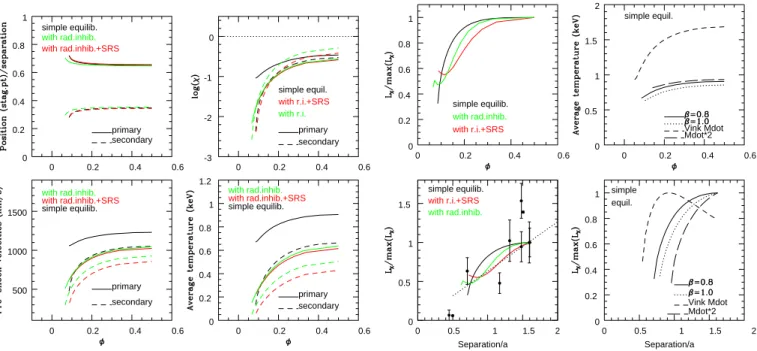
To further investigate this question, we calculated the ex-pected collision parameters in a way similar to that done for Cyg OB2 #9 (Naz´e et al., 2012b). To this end, we considered the stellar and orbital parameters listed in Table 1 (Paper I). We also assume a β-law (with β=0.8) for the wind velocities and re-peated the equilibrium calculation considering radiative inhibi-tion with or without self-regulated shocks (SRS, Parkin & Sim, 2013). The first two columns of Fig. 6 show the predicted col-lision parameters. The equilibrium between the two wind mo-menta is found to occur at about 65% of the separation, counting from the primary star, for φ > 0.1; no equilibrium between the two winds can be found at and close to periastron. In parallel, the pre-shock velocities decrease with phase, leading to a de-crease of at least 40% in the shocked plasma temperature, while observations suggest a smaller variation (see Sect. 4.2). Finally, the cooling parameter χ, which indicates the nature of the colli-sion (> 1 if adiabatic, radiative otherwise; Stevens et al., 1992), suggests that the collision always remains radiative.
In addition, we calculated the expected X-ray luminosities for each colliding wind using the formalism of Zabalza et al. (2011), and summed them to get the evolution with phase of the total X-ray luminosity associated with the collision. The re-sults are shown in the third column of Fig. 6: whatever the case, a maximum at apastron is expected, with a longer recovery after periastron if the effects of radiative inhibition and self-regulated shocks are included. In fact, when plotted relative to separation, theory and observation appear to follow similar trends, espe-cially if the data near φ ∼ 0.65 are excluded. In this context, we note that these predictions are sensitive to the chosen wind parameters. In particular, if the mass-loss rates of the Vink et al. (2000) recipe are used, implying a reduction of the primary value by a factor of two, then the collision becomes adiabatic during more than half the orbit, the temperatures are higher, wind
equi-0 0.2 0.4 0.6 500 1000 1500 primary secondary simple equilib. with rad.inhib.+SRS with rad.inhib. 0 0.2 0.4 0.6 0 0.2 0.4 0.6 0.8 1 1.2 primary secondary simple equilib. with rad.inhib.+SRS with rad.inhib. 0 0.2 0.4 0.6 0 0.2 0.4 0.6 0.8 1 primary simple equilib. secondary with rad.inhib.+SRS with rad.inhib. 0 0.2 0.4 0.6 -3 -2 -1 0 primary secondary simple equil. with r.i.+SRS with r.i. 0 0.2 0.4 0.6 0 0.2 0.4 0.6 0.8 1 simple equilib. with r.i.+SRS with rad.inhib. 0 0.5 1 1.5 2 0 0.5 1 1.5 simple equilib. with r.i.+SRS with rad.inhib. Separation/a 0 0.5 1 1.5 2 0 0.2 0.4 0.6 0.8 1 simple equil. Vink Mdot Mdot*2 Separation/a 0 0.2 0.4 0.6 0 0.5 1 1.5 2 simple equil. Vink Mdot Mdot*2
Fig. 6. Left and Middle panels:Theoretical evolution with phase of the position of the stagnation point, of the pre-shock velocities, of the cooling parameter χ (the dotted line in that panel indicating the limit between radiative and adiabatic collisions), of the average post-shock temperatures (kT ∼ 0.6[v/1000 km s−1]2), and of the X-ray luminosities (compared to their maximum values).
Luminosities are also shown as a function of separation rather than phase. In this panel, observed fluxes in the hard band, corrected for interstellar absorption and normalized by values closest to apastron, are shown with black dots to facilitate comparison with expectations. In the same panel, the best-fit linear relation to the predicted X-ray luminosities (including radiative inhibition and SRS) is added as a dotted line to highlight the predicted trend with separation. Right panels: Comparison of the temperatures (top, as a function of phase for the primary wind) and of the normalized X-ray luminosities (bottom, as function of separation) predicted for simple equilibrium using mass-loss rates from Table 1 with velocities following a β = 0.8 or 1.0 law (solid and dotted lines, respectively), using mass-loss rates derived from the recipe of Vink et al. (2000) with β = 0.8 (short dashed line), or using a mass-loss rate for the primary twice as high as that in Table 1 with β = 0.8 (long dashed line).
librium nearly always occurs, and the X-ray luminosity varies in a very different way, incompatible with observations (see the last column of Fig. 6). Increasing the mass-loss rate of the primary by a factor of two yields less dramatic changes, but the collapse occurs even earlier. The relative strengths of the winds are thus well constrained by the X-ray light curve. However, changing the exponent of the velocity law in simple equilibrium cases to β=1, as is better for supergiants, does not change the predictions much (see last column of Fig. 6). Nevertheless, the observed X-ray light curve is clearly not symmetric around φ = 0.5 as in our simple analytical models. Combined with the too low and vari-able expected temperatures, this underlines the need for a full hydrodynamic model of the system to secure our understanding of the collision in HD 166734.
6. Conclusion
Using Swift and XMM-Newton observatories, we performed an X-ray monitoring of the massive binary HD 166734. It revealed clear evidence of the presence of a wind-wind collision: high flux, presence of a f line combined to the absence of the i lines in triplets of He-like ions, and presence of phase-locked flux vari-ations. The observed changes have three important characteris-tics: (1) a long and deep minimum occurring at and very close to periastron (and to the time of the optical eclipse), (2) asymmet-ric decrease/increase in flux, and (3) a short interval of increasing flux after apastron but before conjunction. The spectral analysis
revealed no significant change in temperature nor absorption: the flux variations are mostly due to changes in the actual emission strength. Because of the long duration and the quasi-constancy of absorption, (wind) eclipse or occultation effects cannot ex-plain the deep flux decrease. When flux variations are compared to the varying separation, a small hysteresis is detected around trends of the form FX ∝dor d2for the hard and soft band,
re-spectively. The collision thus does not appear to be adiabatic in nature. Predictions from analytical models of the collision based on the orbital and stellar parameters of the system indeed favour a radiative nature, and seem to explain the observed trend in X-ray luminosity. The agreement is less good for temperatures (too low and variable in models), and some light curve peculiarities (asymmetric character, with an event between apastron and con-junction keeping the X-ray flux rather high) remain unexplained, calling for more sophisticated modelling as well as complemen-tary observations.
Acknowledgements. We acknowledge support from the Fonds National de la
Recherche Scientifique (Belgium), the Communaut´e Franc¸aise de Belgique, the PRODEX XMM-Newton and Integral contracts, and an ARC grant for concerted research actions financed by the French community of Belgium (Wallonia-Brussels Federation). We thank Norbert Schartel and the ESAC staff, as well as the Swift scientists for their kind assistance that made these observations pos-sible. ADS and CDS were used in preparing this document.
References
Cazorla, C., Naz´e, Y., & Rauw, G. 2014, A&A, 561, A92
Conti, P. S., Ebbets, D., Massey, P., & Niemela, V. S. 1980, ApJ, 238, 184 Corcoran, M. F., Hamaguchi, K., Pittard, J. M., et al. 2010, ApJ, 725, 1528 Corcoran, M.F., Pollock, A.M.T., Hamaguchi, K., & Russell, C. 2011,
arXiv:1101.1422
Gosset E. 2007, Abilitation thesis, University of Li`ege Gosset, E., & Naz´e, Y. 2016, A&A, 590, A113
Gudennavar, S. B., Bubbly, S. G., Preethi, K., & Murthy, J. 2012, ApJS, 199, 8 Hamaguchi, K., Corcoran, M. F., Russell, C. M. P., et al. 2014, ApJ, 784, 125 Leutenegger, M. A., Paerels, F. B. S., Kahn, S. M., & Cohen, D. H. 2006, ApJ,
650, 1096
Lindgren, B.W. 1976, Statistical theory - third edition, McMillan Pub. (New York)
Lomax, J. R., Naz´e, Y., Hoffman, J. L., et al. 2015, A&A, 573, A43
Mahy, L., Damerdji, Y., Gosset, E., Nitschelm, C., Eenens, P., Klotz, A., & Sana, H. 2017, A&A, in press (Paper I)
Mason, B. D., Hartkopf, W. I., Gies, D. R., Henry, T. J., & Helsel, J. W. 2009, AJ, 137, 3358
Naz´e, Y. 2009, A&A, 506, 1055
Naz´e, Y., Broos, P. S., Oskinova, L., et al. 2011, ApJS, 194, 7 Naz´e, Y., Zhekov, S. A., & Walborn, N. R. 2012a, ApJ, 746, 142 Naz´e, Y., Mahy, L., Damerdji, Y., et al. 2012b, A&A, 546, A37
Otero, S. A., & Wils, P. 2005, Information Bulletin on Variable Stars, 5644, 1 Owocki, S. P., & Cohen, D. H. 2001, ApJ, 559, 1108
Pandey, J.C., Pandey, S.B., & Karnakar, S. 2014, ApJ, 788, 84 Parkin, E. R., & Sim, S. A. 2013, ApJ, 767, 114
Pittard, J.M., & Parkin, E.R. 2010, MNRAS, 403, 1657
Pollock, A. M. T., Corcoran, M. F., Stevens, I. R., & Williams, P. M. 2005, ApJ, 629, 482
Porquet, D., Mewe, R., Dubau, J., Raassen, A. J. J., & Kaastra, J. S. 2001, A&A, 376, 1113
Rauw, G., & Naz´e, Y. 2016, Advances in Space Research, 58, 761 Rauw, G., Naz´e, Y., Wright, N. J., et al. 2015, ApJS, 221, 1 Sana, H., Antokhina, E., Royer, P., et al. 2005, A&A, 441, 213 Sana, H., Le Bouquin, J.-B., Lacour, S., et al. 2014, ApJS, 215, 15 Schild, H., G¨udel, M., Mewe, R., et al. 2004, A&A, 422, 177 Stevens, I.R., Blondin, J.M., & Pollock, A.M.T. 1992, ApJ, 386, 265 Sugawara, Y., Tsuboi, Y., & Maeda, Y. 2008, A&A, 490, 259
Vink, J. S., de Koter, A., & Lamers, H. J. G. L. M. 2000, A&A, 362, 295 Waldron, W. L., & Cassinelli, J. P. 2007, ApJ, 668, 456 (erratum ApJ, 680, 1595) Wolff, R. J. 1963, PASP, 75, 485
Zabalza, V., Bosch-Ramon, V., & Paredes, J. M. 2011, ApJ, 743, 7 Zhekov, S. A., Gagn´e, M., & Skinner, S. L. 2014, ApJ, 785, 8