TEST D'HOMOGÉNÉITÉ AVEC LES
L-MOMENTS MULTIVARIÉS
T
EST D'
HOMOGÉNÉITÉ AVEC LESL-
MOMENTS MULTIVARIÉSpar :
F. Chebana* et T.B.M.J. Ouarda
Chaire en hydrologie statistique (Hydro-Québec / CRSNG) Chaire du Canada en estimation des variables hydrologiques
INRS-ETE, Université du Québec
490, rue de la Couronne (Québec), Canada G1K 9A9
Rapport de recherche N° R-933
TABLE OF CONTENTS
TABLE OF CONTENTS...iv
LIST OF FIGURES... v
LIST OF TABLES...vii
ABSTRACT ...ix
1. INTRODUCTION AND LITERATURE REVIEW ... 1
2. THEORETICAL BACKGROUND ... 7
2.1 Multivariate L-moments... 7
2.2 Copulas ... 9
3. DEVELOPMENT OF THE PROPOSED MULTIVARIATE STATISTICS ... 13
3.1 Discordancy test ... 13 3.2 Homogeneity test... 15 4. ADAPTATION TO FLOODS... 19 5. SIMULATION STUDY ...23 6. SIMULATION RESULTS...29 7. CONCLUSIONS... 43 8. ACKNOWLEDGMENTS: ...45 9. REFERENCES ... 47 10. NOTATIONS ...53
LIST OF FIGURES
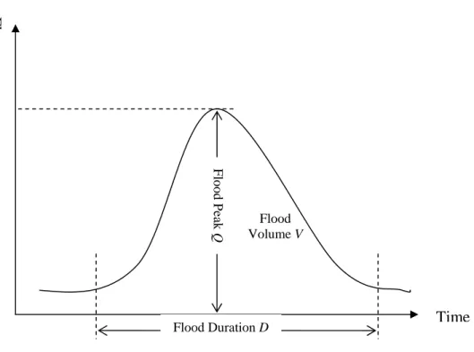
Figure 1. Typical flood hydrograph ...20
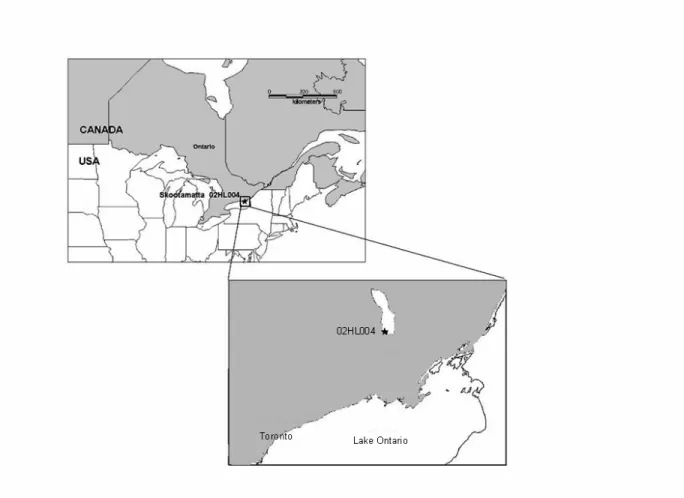
Figure 2. Geographical location of the Skootamatta basin in Ontario, Canada ...24
Figure 3.a. Test power for completely heterogeneous region with n = 30 ...34
Figure 3.b. Test power for marginally heterogeneous region with n = 30 ...345
Figure 3.c. Test power for dependence heterogeneous region with n = 30 ...346
Figure 4. Rates of heterogeneity measure for dependence heterogeneous region with n = 30...37
LIST OF TABLES
Table 1. Flood volume and peak models for some basins considered in the literature ... 20 Table 2. Discordancy values of sites in the described regions, n = 30, N = 20 ... 30 Table 3. Simulation results for homogeneity test when regions are homogeneous, n = 30... 32 Table 4. Simulation results for homogeneity test when regions are 50% heterogeneous
with n = 30 ... 33 Table 5. Simulation results for homogeneity test when regions are 30% bimodal with
n = 30 ... 40 Table 6. Simulation results for homogeneity test when regions are 50% heterogeneous
and variable n from site to site and N = 21 ... 41 Table 7. Simulation results for homogeneity test when n = 60 and N = 30... 42
ABSTRACT
Several types of hydrological events are described with multivariate characteristics (droughts, floods, rain storms, etc.). When carrying out a multivariate regional frequency analysis for these events it is important to jointly consider all these characteristics. The aim of this paper is to extend the statistical homogeneity test of Hosking and Wallis (1993) to the multivariate case. As a tool, multivariate L-moments are used to define the statistics and general copula models to describe the statistical behaviour of dependent variables. The usefulness of the methodology is illustrated on flood events. Monte-Carlo simulations are also performed for a bivariate Gumbel logistic model with GEV marginal distributions. Results illustrate the power of the proposed multivariate L-moment homogeneity test to detect heterogeneity on the whole structure of the model and on the marginal distributions. In a bivariate flood setting, a comparison is carried out with the classical homogeneity test of Hosking and Wallis based on several types of regions.
1. INTRODUCTION AND LITERATURE REVIEW
Hydrologic events are complex and often characterized by the joint behaviour of several random variables, which are not usually independent. Examples of multivariate representation of hydrologic phenomena include storm duration and intensity (Yue, 2001a; Salvadori and De Michele, 2004b); flood peak, volume and duration (Ashkar, 1980; Yue et al., 1999; Ouarda et al., 2000; Yue, 2001b; Yue and Rasmussen, 2002; Shiau, 2003; De Michele et al., 2005; Zhang and Singh 2006); and drought volume, duration and magnitude (Kim et al., 2003; Ashkar et al., 1998). This multivariate understanding of flood, storm or drought event characteristics is essential for several engineering planning, design, and management activities. Multivariate approaches represent these events better than classical univariate tools. Snyder (1962) and Wong (1963) realized the first applications of multivariate analysis tools in hydrological analysis.
A thorough understanding of multivariate hydrological events requires the study of the joint probabilistic behaviour of two or more correlated random variables that characterize the events (Yue et al., 2001). For investigating the statistical behaviour of dependent variables, copulas are recently shown to represent a useful mathematical tool for hydrological applications (El Adlouni et al., 2004; Salvadori and De Michele; 2004a). Several bivariate distributions were considered in the literature for local multivariate studies. For instance, an expression of the joint distribution function of the largest flood peak and its time of occurrence is developed by Gupta et al. (1976). To study rainfall intensity and the corresponding depth, Singh and Singh (1991) derived a bivariate probability density with marginal exponential distributions. Bacchi et al. (1994) modeled extreme rainfall duration and severity by using a bivariate distribution with marginal
exponential distributions. The bivariate normal distribution was investigated by Goel et al. (1998) to represent the joint distribution of flood peaks and volumes based on a partial duration series. To represent the joint probability distribution of flood peaks and volumes and the joint probability distribution of flood volumes and durations, Yue et al. (1999) used the Gumbel mixed model with standard Gumbel marginal distributions. Yue (2001b), Yue and Rasmussen (2002) and Shiau (2003) used the Gumbel logistic model with standard Gumbel marginal distributions to model flood volume and peak for different basins. Salvadori and De Michele (2004b) considered storm duration-intensity using the generalized Pareto distribution with suitable 2-copula Frank’s family. In the study by El Adlouni et al. (2004) several copulas are considered to model flood peak and volume with respectively Gumbel and Gamma marginal distributions.
Regional frequency analysis is commonly used for the estimation of extreme hydrological events, such as floods, at sites where little or no data are available. It allows to utilize data available from other stations in the same hydrologic region. In general a regional flood frequency procedure consists of two steps: delineation of hydrological homogeneous regions and regional estimation. This subject was investigated by several studies including Stedinger and Tasker (1986), Burn (1990), Hosking and Wallis (1993), Durrans and Tomic (1996), Nguyen and Pendey (1996), Alila (1999, 2000). GREHYS (1996a,b) presented the results of an intercomparison of various regional flood estimation procedures obtained by coupling four methods for delineating homogenous regions and seven regional estimation methods.
The size of a region is a factor that is closely related to the notion of degree of homogeneity. Indeed, the consideration of a region with few sites guarantees its high degree of homogeneity. However, in such a situation, the available data may not be sufficient to carry out a suitable
regional estimation. On the other hand, large regions may contain some dissimilar sites to the target one. In the region of influence approach (ROI), Burn (1990) proposed three options to select a threshold value combined with a weight function in order to define a convenient homogeneous region for a given site. Using a jack-knife resampling procedure, Ouarda et al. (2001) proposed to address this problem by optimizing the relative bias and the relative mean square error of quantile estimates. Hosking and Wallis (1993) proposed a procedure to deal with the issue of homogeneity testing in the univariate framework. Their procedure consists of three statistics to measure the discordancy of sites, the heterogeneity of the region and the goodness-of-fit of the regional distribution. The proposed statistics are defined on the basis of the L-moments of local data (Hosking, 1990).
Most literature related to multivariate representation of hydrological phenomena dealt with at-site (local) multivariate frequency analysis of hydrological events. Very little effort has been devoted to the joint representation of the characteristics of hydrological events in regional hydrological modeling at ungauged sites. Joint regional study of flood peaks and volumes using a canonical correlation analysis procedure was carried out by Ouarda et al. (2000) in the province of Quebec, Canada. It is possible to carry out a regional frequency analysis for each variable of the event, each having its own homogeneous region. However, it is of interest to identify a single homogeneous region for which the given variables have approximately the same joint distribution across sites. Univariate regional hydrological frequency analysis can only provide limited evaluation of these events at ungauged sites and is not sufficient to fully represent multiple hydrological event phenomena.
It is possible to treat the problem of testing the homogeneity of a region with several characteristics, from a statistical point of view, by using either one multivariate test or a series of
univariate tests. One important aspect of the use of a multivariate test in opposition to the use of a series of univariate tests concerns the control of first kind errors. If p independent univariate tests are carried out, each of which at the 5% significance level, then the probability of getting a
non significant result is0.95 .p Therefore, the probability of getting at least one significant result is
(1 0.95− p), which may be unacceptably large. On the other hand, a multivariate test using the 5% level of significance gives a 0.05 probability of first kind error, independently of the number of involved variables. This is a distinct advantage over a series of univariate tests, particularly when the number of variables is large. It can also be argued that the use of a single multivariate test provides a better procedure in many cases than making a large number of univariate tests. A multivariate test has also the additional advantage of taking proper account of the correlation between variables (See Manly, 2005).
The aim of the present paper is to extend the discordancy statistic and the homogeneity test of Hosking and Wallis (1993) to the multivariate case. This is considered as an important step in regional frequency analysis of multivariate events, and consists in testing whether a region is homogeneous or heterogeneous. A multivariate version of L-moments, defined by Serfling and Xiao (2006), is used to develop the multivariate discordancy and homogeneity statistics. The multivariate nature of hydrological events is modeled using copulas.
In the univariate context, Hosking and Wallis (1993) consider the index flood model originally proposed by Dalrymple (1960) for regional estimation. It is based on the assumption that floods at different sites within a region are identically distributed except for a scale factor. Hosking and Wallis (1993) treat their statistic as a heterogeneity measure. Therefore, they judge its performance with the evaluation of the relative root mean square error (RRMSE) of quantile estimates in an index flood model. However, Fill and Stedinger (1995) used the Hosking-Wallis
statistic as a statistical test to examine homogeneity and they evaluated its power for comparison with other tests. In this paper, both potential uses of the statistics are considered: homogeneity test and heterogeneity measure. Hence, the evaluation of the performance of the proposed tests is two folds: On one hand the power is used as a criterion when it is treated as a statistical homogeneity test, and on the other hand the occurrence rates of three kinds of regions (homogeneous, acceptably homogeneous and definitely heterogeneous) is used when it is treated as a heterogeneity measure. Recall that the power of a statistical test is the probability that a sample falls in the critical region when the alternative hypothesis is true. The reasons for this choice are: (a) a multivariate version of the index flood model has yet to be developed to allow the computation of quantiles and consequently their RRMSE, and (b) the evaluation based on quantiles RRMSE evaluates the whole regional frequency analysis procedure (the homogeneity test as well as the parameter and quantile estimation method). Consequently, when a result is not satisfactory, in the RRMSE sense, one can not identify the source of the poor performance which may be caused by the homogeneity test, the model or the parameter estimation method.
Monte Carlo simulations are drawn to validate and evaluate the results. The selected bivariate model for the local joint variable volume-peak is the Gumbel logistic model with Gumbel marginal distributions. Several kinds of heterogeneous regions are generated. When the generated regions are homogeneous, the parameters of the model are approximately those of the Skootamatta basin in Ontario, Canada (Yue and Rasmussen, 2002).
The paper is organized as follows. In Section 2, a short discussion of the theoretical background is presented: multivariate L-moments and copulas. The theoretical developments of the discordancy and homogeneity tests are presented in Section 3. Section 4 deals with the adaptation of the approach to flood events. The simulation experiment is presented in Section 5,
and Section 6 deals with the discussion and interpretation of results. Concluding remarks are presented in the last section.
2. THEORETICAL BACKGROUND
In this section the mathematical tools needed for the development of the multivariate homogeneity and discordancy tests are briefly presented. All notations used in the following are reported in Section 10.
2.1 Multivariate L-moments
The L-moment approach offers strong advantages for the modeling of heavy-tailed distributions such as some of the distributions used in hydrology. The properties and advantages of L-moments are presented in Hosking and Wallis (1997). Multivariate L-L-moments are principally developed by Serfling and Xiao (2006). In the following the bivariate L-moment case is briefly presented.
LetX( )j be a random variable with distributionF , for j=1,2. By analogy with a covariance j
representation of L-moments of order k ≥1, multivariate L-moments are matrices Λ with L-k
comoment elements defined by:
(
)
(
( ) * ( ))
[ ] Cov , 1 ( ) , , 1,2 and 2,3,... i j k ij X Pk F Xj i j kλ
= − = = (1)whereP is the so-called shifted Legendre polynomial. Note that the elements k* λk ij[ ] and λk ji[ ]are not necessarily equal. Particularly, the first L-comoment elements are:
(
)
(
)
(
)
(
) (
)
(
)
(1) ( 2) 2[12] 2 2 (1) ( 2) 3[12] 2 3 (1) (2) ( 2) 4[12] 2 2 2Cov , ( ) 6Cov , ( ) 1/ 2 Cov , 20 ( ) 1/ 2 3 ( ) 1/ 2 1 X F X X F X X F X F X λ λ λ = = − = − − − + (2)which are respectively the L-covariance, L-coskewness and L-cokurtosis.
Note that the kth L-comoment of X(1) with respect to X( 2)is translation invariant and scale
equivariant with respect to transformations of (1)
X and translation and scale invariant with
respect to transformations ofX( 2); that is for positive b and d, and arbitrary a and c, it satisfies:
(1) (2) (1) (2)
[12]( , ) [12]( , )
k a b X c d X b k X X
λ + + = λ (3)
The L-comoment coefficients are given by
[12] [12] (1) 2 , for 3 k k k
λ
τ
λ
= ≥ and 2[12] 2[12](1) 1λ
τ
λ
= (4) where ( ) [ ] j k k jjλ
=λ
is the classical kth L-moment of the variable X( )j , 1, 2j= as defined by Hosking (1990).A hierarchy of intuitively appealing analogues of the classical covariance and the central comoments is thus provided by L-comoments. Their interpretations and comparisons are
facilitated by the fact that they are defined in terms of the classical covariance operator. The matrix of the L-comoment coefficients is written as
( )
[11] [12] * [ ] , 1,2 [21] [22] k k k k ij i j k kτ
τ
τ
= ⎛τ
τ
⎞ Λ = = ⎜ ⎟ ⎝ ⎠ (5)Particularly, for k=2 the L-covariation matrix is given by: 2[11] 2[12] * 2 2[21] 2[22] τ τ τ τ ⎛ ⎞ Λ = ⎜ ⎟ ⎝ ⎠ (6)
and for k = 1, the first order bivariate L-moment corresponds to the mean vector
(1) ( 2)
1 ( , )
t
E X X
λ
= .As indicated by Serfling and Xiao (2006), the L-comoments are similar in structure and behavior
to the univariate L-moments and capture their attractive properties.
The multivariate L-moments defined previously are based on a theoretical population
distribution; however their finite sample versions are useful to define statistical tests and also to estimate multivariate distribution parameters. Their formulas and properties are presented in Serfling and Xiao (2006). In the R software package, William (2006) proposes an
implementation of these finite sample versions.
2.2 Copulas
To overcome the limitations of classical dependence measures, copulas have recently received increasing attention in various science fields (see for instance Nelsen, 1999). Copula is a description and a model of the dependence structure between random variables, independently of the marginal laws. The general development of copulas theory can be found in Nelsen (1999). A copula is a function C: I× → (I = [0, 1]) such that: I I
• for all u, v I∈ : C(u, 0) = 0, C(u, 1) = u, C(0, v) = 0, and C(1,v) = v; • for all u u1, , v , v2 1 2∈ such that I u1 ≤u2 and v1≤v2:
2 2 2 1 1 2 1 1
( , v ) ( ,v ) ( , v ) ( , v ) 0
C u −C u −C u +C u ≥ (7)
The link between copulas and bivariate distributions is provided by the following Sklar’s (1959) result which states that the most general marginal-free description of the dependence structure of
multivariate distributions is through its copula: Let F1 and F denote the marginal distribution 2
functions of the random variables (1)
X and ( 2)
X , let F be a joint distribution function with 1,2
marginals F1 and F . Then, there exists a copula C such that, for all real 2 x and 1 x , we have: 2
(
)
1,2( ,1 2) 1( ), (1 2 2)
F x x =C F x F x (8)
if F1 and F are continuous, then C is unique. 2
Archimedean and Extreme Value copulas represent classes of particular interest. The class of
extreme-value copulas arises as the possible limit of copulas of the variable
(
Mn1,Mn2)
where (1) ( 2) 1 2 1 1 max , max n i n i i n i n M X M X ≤ ≤ ≤ ≤ = = and(
(1) ( 2))
1 , i i i n X X≤ ≤ is a bivariate sample of independent
and identically distributed random variables. A useful representation proposed by Pickands (1981) facilitates the use of bivariate extreme-value copulas. Formally, a copula C is an
extreme-value copula if and only if there exists a real-extreme-valued function A on the interval [0, 1] such that:
(
)
log( , ) exp log log , 0 , 1
log log u C u v u v A u v u v ⎧ ⎛ ⎞⎫ = ⎨ + ⎜ ⎟⎬ < < + ⎝ ⎠ ⎩ ⎭ (9)
The case A≡ corresponds to independence, and 1 A t( )=max ,1
{
t −t}
corresponds to the copula ( , ) min( , )C u v = u v . Statistical inference on Pickand’s function A can summarize the inference on
its bivariate extreme-value copula C.
A bivariate Archimedean copula is characterized by a generator (.)ψ that is a convex decreasing function satisfying (1)ψ = where: 0
(
)
1
( , ) ( ) ( ) , 0 , 1
C u v =
ψ ψ
− u +ψ
v <u v< (10)Copulas that belong to this class are symmetric and associative.
A simple and popular model is the Gumbel logistic model, where the corresponding copula is the only one to meet at the same time the conditions of the extreme-value copula with:
(
)
1/( ) m (1 )m m, 1
A t = t + −t m≥ (11)
and the conditions of Archimedean copulas with:
(
)
( )t logt m, 1m
3. DEVELOPMENT OF THE PROPOSED MULTIVARIATE
STATISTICS
In this section, the proposed multivariate discordancy and homogeneity tests are presented in their general forms. It is important to note that, before proceeding with the multivariate regional procedure, it is advisable to test the independence between variables. The reader is referred to Ondo et al. (1997) for a review of such tests. In the case of independence, it is sufficient to use several univariate Hosking and Wallis (1993) tests according to the number of variables.
3.1 Discordancy test
The assessment of the discordancy measure of a site i among a set of N sites is a preliminary step before proceeding with the homogeneity analysis.
In the following the discordancy test proposed by Hosking and Wallis (1993) is extended to the
multivariate framework. For this purpose, the matrix Uit = Λ⎡⎣ 2*(i) Λ3*(i) Λ* (i)4 ⎤⎦ is considered for
each site i. It contains the three matrices Λ*(i)2 , Λ*(i)3 and Λ defined in equations (5) and (6). The * (i)4 following matrix Diis defined by:
(
) (
1)
1 3 t i i i D = U −U S− U −U (13) where(
)(
)
1 1 ( 1) N t i i i S N − U U U U = = −∑
− − (14)1 1 N i i U N− U = =
∑
(15)and At is the transpose of a matrix or a vector A.
The number 3 appearing in the denominator of expression (13) can be replaced by the value 12
which represents the number of elements in the three matrices *(i) *(i) * (i)
2 , 3 and 4
Λ Λ Λ , and it can be seen as the number of degrees of freedom of the chi-square distribution. However, simulations show that the use of the value 12 reduces the discordancy statistic values and prevents it to make discordant sites more evident.
In order to evaluate the discordancy of a site i, it is possible to use a norm Di of the matrixDi.
This transformation from the multidimensional space to the real line has the advantage of defining an intuitive distance in the vector space and reducing exactly to the usual univariate case.
Several matrix norms can be used for this purpose. For instance, the maximum absolute column
sum norm A1of a matrix A with elements a is defined as: ij
1 max ij
j i
A =
∑
a (16)The spectral norm A2 is the square root of the maximum eigenvalue of A At :
t
2 maximum eigenvalue of
A = A A (17)
The maximum absolute row sum norm is defined by:
max ij
i j
Finally, the Frobenius norm, sometimes called the Euclidean norm, is given by: , trace of t ij F i j A =
∑
a = A A (19)The reader can consult Horn and Johnson (1990) for more details about the matrix norms. These various matrix norms are tested in the simulation study of the present work.
A site i is discordant, with respect to the considered set of sites, if Di takes large values, where
. is one of the abovementioned norms. As a critical value for Di , the constant
1 0.05(3) 3 2.6049
c= χ− = may be considered for large regions, where χ1−α( )d is the quantile of a chi-square distribution of order α with d degrees of freedom.
As indicated in Hosking and Wallis (1997), it is advisable to examine the data for the sites with
the largest Di values, regardless of the magnitude of these values. Special attention should be
given to the definition of the critical value taken for small regions. For instance, these constants may be obtained for finite sample sizes by the use of the bootstrap technique, see e.g. Efron and Tibshirani (1994).
3.2 Homogeneity test
The proposed homogeneity test is described as a multivariate analogue of the statistic given by
Hosking and Wallis (1993). Following the same logic as in the above section, the statistic V. is
defined as: 1/ 2 1 2 * ( ) * 2 2 . 1 1 N N i i i i i V n n − = = ⎛⎛ ⎞ ⎞ =⎜⎜⎜ ⎟ Λ − Λ ⎟⎟ ⎝ ⎠ ⎝
∑
∑
⎠ (20)where . is one of the norms defined above, 1 * * ( ) 2 2 1 1 N N i i i i i n n − = = ⎛ ⎞ Λ =⎜ ⎟ Λ ⎝
∑
⎠∑
and * ( ) 2 i Λ defined in (6) is the L-covariation coefficient matrix for site i, with record length n , 1,...,i i= N. When handling only one variable the statistic V. reduces to the V statistic of Hosking and Wallis (1993)whatever the norm taken.
Similarly to the univariate case, the observed value of the statisticV. is standardized using the
mean and standard deviation values of V. computed on the basis of a large number of simulated
homogeneous regions. Hence, the statistic that measures the heterogeneity of a set of sites is given by: . . Vsim Vsim V H μ σ − = (21)
where μVsim and σVsimare the mean and standard deviation of the Nsim values of V.of simulated regions. The simulated regions are homogeneous with sites having the same record lengths as their observed counterparts. To avoid any subjective choice of the bivariate distribution on which
the simulations are carried out to compute μVsim and σVsim, this bivariate distribution should be as general as possible and include most distributions commonly used in hydrology.
Recall that in the univariate setting, a kappa distribution with 4 parameters is simulated by Hosking and Wallis (1993). If it exists, the extension of this distribution to the multivariate case requires a large number of parameters. Indeed, this distribution would possess at least 4 parameters for each variable along with the covariance parameters. To overcome these difficulties related to classical dependence measures, copulas are used at this level. In hydrology,
particular classes of copulas are defined: the extreme-value copulas characterized by a dependence function A, and the Archimedean copulas determined by a generator functionψ . The dependence function A may be estimated by several nonparametric methods existing in the
literature. The reader is referred to Segers (2004) for a review of these methods. On the other hand, a convenient choice behind the bivariate extreme value copula is the four parameter kappa distribution for the marginals. These marginal distributions do not necessarily need to be from the same family. Aside from avoiding the subjective choice of a distribution, this avoids committing errors in the goodness of fit test along with errors of parameter estimation of the fitted distribution.
In order to generate samples from the variables
(
X(1),X( 2))
according to extreme value copula with a general setting of the function A, Ghoudi et al. (1998) developed an algorithm of specialinterest when performing simulations. To summarize this algorithm, let U1, U be uniform 2
random variables and Z be a random variable with a cumulative distribution function G and Z
probability density function g where Z G zZ( )= +z z(1−z A z) '( ) / ( ),A z 0≤ ≤z 1.This algorithm consists of the following steps:
1. Simulate Z.
2. Given Z, take W =U1with probability ( )p Z and W =U U1 2with probability 1−p Z( ), where p z( )= z(1−z A z) ''( )
(
A z g( ) Z( ) .z)
It is important to take into consideration the numerical nonparametric smoothing when using this algorithm in practice, since it is also based on the first and second derivatives of the function A.
Despite the general validity of this procedure, extra information about the model, e.g. parametric form of A, can be useful to increase the speed and accuracy of the generation algorithm.
Depending on the value of H. a decision concerning the homogeneity of the observed region
can be taken. Two scenarios can then be considered. In the first scenario, H. is considered as a
statistical homogeneity test with first kind error 5%, as in Fill and Stedinger (2004) for univariate distributions. The rejection region of the homogeneity is then H. >1.64. In the second scenario,
.
H is considered as a measure of heterogeneity, as in Hosking and Wallis (1993). In this case, a
region of sites is declared to be homogeneous if H. <1, acceptably homogenous if 1<H. <2
and definitely heterogonous ifH. >2.
The extension of the univariate heterogeneity measure considered here concerns only the LCV measure of variation. Other measures used in Hosking and Wallis (1993) can also be considered for the extension by following the same procedure and using the same tools.
4. ADAPTATION TO FLOODS
The discordancy and homogeneity tests defined in the previous section are general and can be applied to several hydrological phenomena such as floods, droughts and rain storms. In this section, the focus is on flood events as multivariate random events that are characterized by their peak Q, volume V and duration D. These combined characteristics determine the severity of a
flood and can be correlated. Figure 1 illustrates a typical hydrograph with these characteristics. In general, there exists a close correlation between flood peak and volume and between food volume and duration, but there is little significant correlation between flood peak and duration, as noticed by Yue (2001b). Without loss of generality, the bivariate vector ( , )V Q is considered
in this study. In order to proceed to simulations, the joint distribution of the random vector ( , )V Q must be determined. In the remainder of the study, the univariate homogeneity tests for
flood volumes and peaks are respectively denoted by HV and H , and also the corresponding Q
discordancy statistics are Di V, and Di Q, for a site i.
In practice, flood peaks and flood volumes may be marginally represented by the Gumbel distribution, as illustrated by previous studies of real data from several sites. In Table 1, the cases studied by Yue et al. (1999), Yue (2001b), Yue and Rasmussen (2002) and Shiau (2003) are summarized. In the present study, both volume and peak variables are considered Gumbel marginally distributed. The Gumbel cumulative distribution function is given by:
( )
{
}
( ) exp exp x , real, 0 and real
Figure 1. Typical flood hydrograph
Table 1. Flood volume and peak models for some basins considered in the literature
α β model m and ρ Reference Basin n
Q (m3/s) 269.3 479.6 V (day.m3/s) 512.6 1256.7 Gumbel logistic m =1.294 ρ=0.403 Shiau (2003) Pachang river,
Taiwan (small basin) 39 Q (m3/s) 15.85 51.85
V (day.m3/s) 300.22 1239.8
Gumbel logistic
m =1.414
ρ =0.5 Yue and Rasmussen (2002)
Skootamatta,ON, CA 41 Q (m3/s) 34.43 168.43 V (day.m3/s) 2287 11106 Gumbel logistic m =1.969 ρ=0.742 Yue (2001b) Harricana, QC, CA 63 Q (m3/s) 280.5 1265 V (day.m3/s) 9707 46602 Gumbel*
mixed ρ=0.596 Yue et al. (1999)
Ashuapmushuan, QC,
CA 33
*
This model is not defined with a parameter m.
Flood Volume V Flow Time Flood Duration D Fl oo d Peak Q
The dependence between V and Q may be modeled by the so-called Gumbel logistic model, expressed according to the following copula:
{
1/}
( , ) exp ( log )m ( log )m m , 1 and 0 , 1 m
C x y = − −⎡⎣ x + − y ⎤⎦ m≥ ≤x y≤ (23)
where m is the dependence parameter, which is related to the correlation coefficient ρ by the relationship m=1/ 1−ρ, 0≤ <ρ 1. Fortunately, the corresponding Gumbel logistic copula
m
C is an extreme value copula with dependence function A t( )=
(
(1−t)m+tm)
1/m and it is also an Archimedean copula with generator function ψ( )t = −(
logx)
m.Zhang and Singh (2006) showed the superiority of the Gumbel logistic copula for modeling the flood volume and peak distribution, using the Akaike Information Criterion (AIC). They compared its performance with four other kinds of copulas and also with non-copula models such as the mixed Gumbel model and the Cox-Box transformation. The Gumbel logistic model is also considered by De Michele et al. (2005) with Frechet extreme value marginal distributions. The marginal distributions are not necessarily the same which is one of the advantages of copula modeling. An example of such situation is treated by El Adlouni et al. (2004).
5. SIMULATION STUDY
The objective of the simulation study is to evaluate the performance of the proposed
homogeneity test H. defined by equation (21) as well as to illustrate the use of the discordancy
statistic Di where Diis given by (13).
Once the model is defined by the marginal distributions (22) and the copula (23), the corresponding parameters must be specified. The parameters selected for simulation study are those of the Skootamatta basin in Ontario, Canada (Yue and Rasmussen, 2002). Figure 2 illustrates the geographical location of the Skootamatta basin in the province of Ontario, Canada. The gauging station 02HL004 is near the outlet of the basin at latitude 44.5494 N and longitude
77.3292 W. A homogenous region with parameters αV =300, βV =1240,αQ =16, 52βQ = and
1.41m= (which is equivalent to ρ =0.5) is hence defined.
The steps of the simulation concerning the homogeneity tests are presented herein. Several elements of the procedure are inspired by Hosking and Wallis (1993):
1. Simulation of regions: Generate a region for both variables volume V and peak Q with N
sites (N = 10, 15, 20 and 30) and a fixed record length ni = =n 30for each site i. In order to study the impact of the record length on the performance of the tests, the case
60 i
n = =n is investigated for N =30. Four cases are also considered when the record length is variable from site to site with N =21: 10,12,...,50ni = ; ni =50, 48,...,10;
10,14,...,50, 46,...,10 i
Figure 2. Geographical location of the Skootamatta basin in Ontario, Canada
To generate heterogeneous regions, without loss of generality, the location parameter
βin the Gumbel marginal distributions (22) is fixed since V is location invariant, and then different values of the parametersα αV, Q and mare considered. The variation of these parameters in the same region suggests several types of regions to be generated, and the following are selected:
b. Completely heterogeneous: All parameters increase linearly from the first to the
Nth site in the 50% range centered around the homogeneous region parameters,
e.g., for αV =300 the variation is in the range
[
300(1- 0.5 / 2), 300(1 0.5 / 2)+] [
= 225, 375]
.c. Heterogeneous on the marginal parameters: It is the same as the above region but the dependence parameter m is fixed and the variation is on the parametersαV and αQ.
d. Heterogeneous on the dependence parameter: The marginal parameters
and
V Q
α α are fixed and the variation is on the dependence parameter m. This region is marginally homogenous.
e. Completely bimodal: Two groups of parameters are defined by the two limits of a 30% range centered on the parameters of the homogeneous region; half the sites have high values of all parameters α αV, Q and m while the other half have low values of these parameters, e.g., for αV =300 the lower value is
300(1- 0.3 / 2)=255 and the higher one is 300(1 0.3 / 2)+ =345.
f. Bimodal on the marginal parameters: The dependence parameter m is fixed and
the marginal parameters αV and αQtake the two sided values similarly to the above region.
g. Bimodal on the dependence parameter: It is the same as the completely bimodal
region with fixed marginal parameters αV and αQ and the dependence parameter
In order to generate a bivariate Gumbel logistic sample with uniform marginal distributions, the algorithm of Ghoudi at al. (1998) described in section 3.2 is used.
Then, the desired sample is obtained with the quantile transformation F−1of the marginal distributions.
2. Computation of the homogeneity statistics: Assess the H statistics HV, HQ and H. with
each norm, on P = 100 generated regions as in step 1. Note that no significant differences have been observed with other values of P such as P = 150 or 200.
3. Performance evaluation: The rates of the values of each statistic H
(
H., HV or HQ)
found in step 2 are computed according to the corresponding conditionsto be satisfied. The rate is the ratio of the number of samples where the H value satisfies the desired condition to the total number of generated samples. That means, when the statistic is considered as a homogeneity test, its power is computed, that is the rate of
1 . 6 4
H > ; and when it is considered as a heterogeneity measure, the rates of the occurrences 1, H < 1 <H < and 2 H > are computed. 2
It is important to note that it is advised to use a kappa distribution to simulate the marginals. However, in the simulation study to evaluate the performances of the tests a Gumbel distribution is used. This is justified by the fact that the treated characteristics are specific variables and the "real regions to be tested" are simulated. Hence, sources of error are reduced since there is no goodness-of- fit testing or parameter estimation. Note that Hosking and Wallis (1993) used the GEV distribution rather than kappa to evaluate the performance of their test in a general univariate framework.
In order to illustrate the discordancy measure Di , regions are simulated which contain N =2 0
sites each of which with record lengthn=3 0. Due to space limitations, the exercise was not carried out for all cases of regions and values of n and N. On the basis of P = 100 generated
regions for each case, the mean values of Di V, , Di Q, and Di for each site are computed. In the
generated regions, all sites have the same parameters as the homogenous region a in the previous procedure except some discordant sites (sites number 1, 6, 11 and 16). These sites have different parameter values. Parameter values of these sites equal ten times the values of the other sites. The difference in these sites concerns all parameters (complete discordancy), marginal parameters (marginal discordancy) and only the dependence parameter (dependent discordancy). A set of P = 100 homogeneous regions is also generated for comparison.
6. SIMULATION RESULTS
The discordancy measure indicates the sites with gross errors that may cause the heterogeneity in
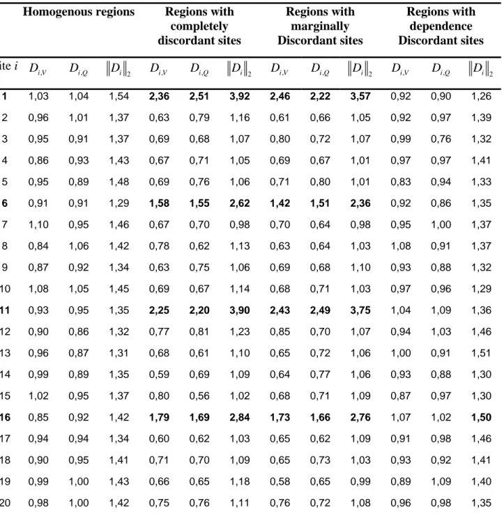
the generated regions. Table 2 illustrates the discordancy values Di V, , Di Q, and Di 2of sites in the
described regions for n=3 0 and N =2 0. Only results with the spectral norm .2 are presented since no significant difference with the other norms is observed. Results in Table 2 show that for the homogenous regions all sites have approximately the same values of the discordancy statistics in both univariate and bivariate cases. When the discordant sites are affected on all parameters, the six supposed discordant sites are detected with higher values of the bivariate statistics than the univariates which have close values. This is due to the fact that, in the bivariate samples, the dependence parameter m causes more discordancy. When the discordancy affects the marginal parameters, the six sites are detected also, with a slightly lower values in the bivariate cases compared to those of completely discordant sites. Finally, when the discordancy affects only the dependence parameter, none of the six sites is detected by the univariate statistics where the values are similar to homogeneous regions; whereas the bivariate statistic detects only one site among the six supposed to be discordant. This can be explained by the fact that there are no differences between sites on the marginals, and the discordancy caused by the dependence parameter alone is not enough to be detected by the discordancy test since it represents little information compared to all the information given by the remainder of non affected parameters.
Table 2. Discordancy values of sites in the described regions, n = 30, N = 20
Homogenous regions Regions with completely discordant sites Regions with marginally Discordant sites Regions with dependence Discordant sites Site i Di V, Di Q, 2 i D Di V, Di Q, Di 2 Di V, Di Q, Di 2 Di V, Di Q, Di 2 1 1,03 1,04 1,54 2,36 2,51 3,92 2,46 2,22 3,57 0,92 0,90 1,26 2 0,96 1,01 1,37 0,63 0,79 1,16 0,61 0,66 1,05 0,92 0,97 1,39 3 0,95 0,91 1,37 0,69 0,68 1,07 0,80 0,72 1,07 0,99 0,76 1,32 4 0,86 0,93 1,43 0,67 0,71 1,05 0,69 0,67 1,01 0,97 0,97 1,41 5 0,95 0,89 1,48 0,69 0,76 1,06 0,71 0,80 1,01 0,83 0,94 1,33 6 0,91 0,91 1,29 1,58 1,55 2,62 1,42 1,51 2,36 0,92 0,86 1,35 7 1,10 0,95 1,46 0,67 0,70 0,98 0,70 0,64 0,98 0,95 1,00 1,37 8 0,84 1,06 1,42 0,78 0,62 1,13 0,63 0,64 1,03 1,08 0,91 1,37 9 0,87 0,92 1,34 0,63 0,75 1,06 0,69 0,68 1,10 0,93 0,88 1,32 10 1,08 1,05 1,45 0,69 0,67 1,14 0,68 0,71 1,03 0,97 0,96 1,29 11 0,93 0,95 1,35 2,25 2,20 3,90 2,43 2,49 3,75 1,04 1,09 1,36 12 0,90 0,86 1,32 0,77 0,81 1,23 0,85 0,70 1,07 0,94 1,03 1,46 13 0,96 0,87 1,31 0,68 0,61 1,10 0,65 0,72 1,06 1,00 0,91 1,51 14 0,99 0,89 1,35 0,59 0,69 1,09 0,64 0,77 1,06 0,93 0,88 1,30 15 1,02 0,95 1,37 0,80 0,56 1,02 0,68 0,71 1,09 0,87 0,97 1,30 16 0,85 0,92 1,42 1,79 1,69 2,84 1,73 1,66 2,76 1,07 1,02 1,50 17 0,94 0,94 1,34 0,60 0,62 1,03 0,65 0,62 1,09 0,91 0,98 1,46 18 0,90 0,95 1,41 0,71 0,70 1,09 0,65 0,73 1,03 0,93 0,92 1,41 19 0,99 1,00 1,43 0,66 0,65 1,18 0,58 0,65 0,99 0,89 1,09 1,40 20 0,98 1,00 1,42 0,75 0,76 1,11 0,76 0,72 1,08 0,96 0,98 1,35
Numbers written in bold character in the first column indicate prior discordant sites, in the other columns they represent the detected discordant sites.
Tables 3 to 7 present the simulation results for homogeneity testing for all configurations of regions and for the various values of n and N. Selected illustrations of the test power and the
rates of heterogeneity measure are presented respectively in Figures 3.a to 3.c and Figure 4 for
the considered regions and for n=3 0. The statistic H.
∞ corresponding to the . ∞norm leads
almost always to the lowest power value among the various statistics H.. The corresponding
loss of power may reach 20%; nevertheless, H.
∞leads to relatively good performances under
homogeneity. Due to space limitations, results about H.
∞are not presented in Figures 3.a-3.c.
Given the similarity in the results of
1 2 . , . and . F H H H , only results of 2 . H are presented in Tables 3-7.
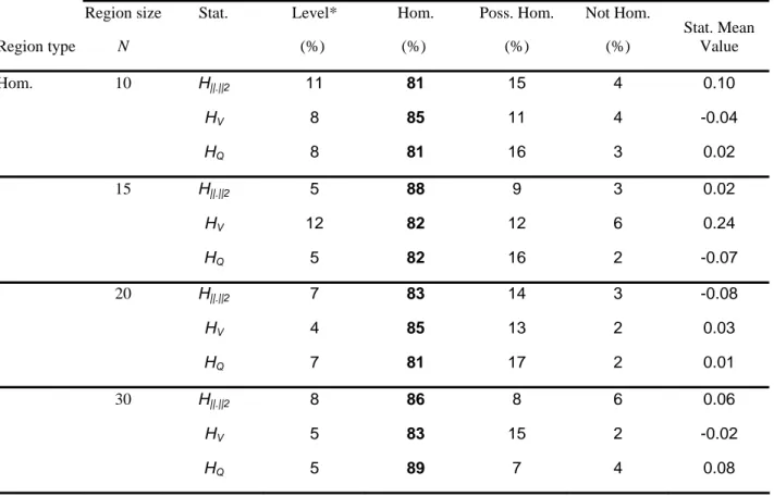
In the case of generated homogeneous regions, the levels (first kind errors) of the H statistics are presented in Table 3. The H statistics mean values are close to zero even for small regions
(
N =1 0)
and the regions are actually identified to be homogeneous. More than 81% of the samples are identified to be homogeneous with both univariate and bivariate statistics. Therefore, there are no significant differences between the results of the univariate and bivariate tests. Note that, occasionally, small negative values of the H statistics are obtained for homogeneous regions. From the relation (21), this may happen when the region is less dispersed, in the sense of.
V , than what would be expected from the simulated homogeneous regions that serve to
compute μVsim.
Results concerning the three 50% heterogeneous regions with record length sites n=30are presented in Table 4. For a given region with size N, the power, the rates and the statistic mean values are presented for each statistical test H. The corresponding powers are illustrated in Figures 3.a-3.c and the occurrence rates of the heterogeneity on the dependence are presented in Figure 4. Similar figures can be produced from Table 4.
Table 3. Simulation results for homogeneity test when regions are homogeneous, n = 30 Region type Region size N Stat. Level* (%) Hom. (%) Poss. Hom. (%) Not Hom. (%) Stat. Mean Value Hom. 10 H||.||2 11 81 15 4 0.10 HV 8 85 11 4 -0.04 HQ 8 81 16 3 0.02 15 H||.||2 5 88 9 3 0.02 HV 12 82 12 6 0.24 HQ 5 82 16 2 -0.07 20 H||.||2 7 83 14 3 -0.08 HV 4 85 13 2 0.03 HQ 7 81 17 2 0.01 30 H||.||2 8 86 8 6 0.06 HV 5 83 15 2 -0.02 HQ 5 89 7 4 0.08
Stat.: Statistic. Hom.: Homogeneous. Poss. Hom.: Possibly Homogeneous.
*Under the homogeneity, the computed probability corresponds to the empirical first kind error.
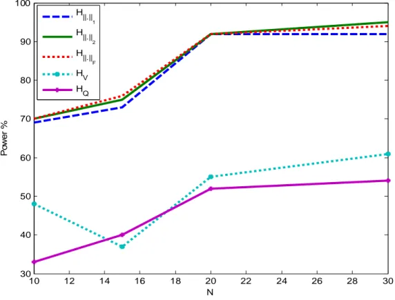
For the completely heterogeneous regions and for any fixed N, the mean value of
2
.
H is larger
than those of HV and HQ as can be seen in the first part of Table 4. Using
2
.
H , with mean
values larger than 2, the region is correctly indicated to be definitely heterogeneous even for
small values of N. In contrast, the univariate statistics HV and HQ, with mean values between
1.36 and 2, wrongly indicate that the region is possibly homogeneous. From Figure 3.a, the
bivariate tests H. lead to equivalent powers which increase from 70% to 90% with respect to N.
The power of both HV and HQ increases also but in the range 30%-60%. This indicates the
superiority of
2
.
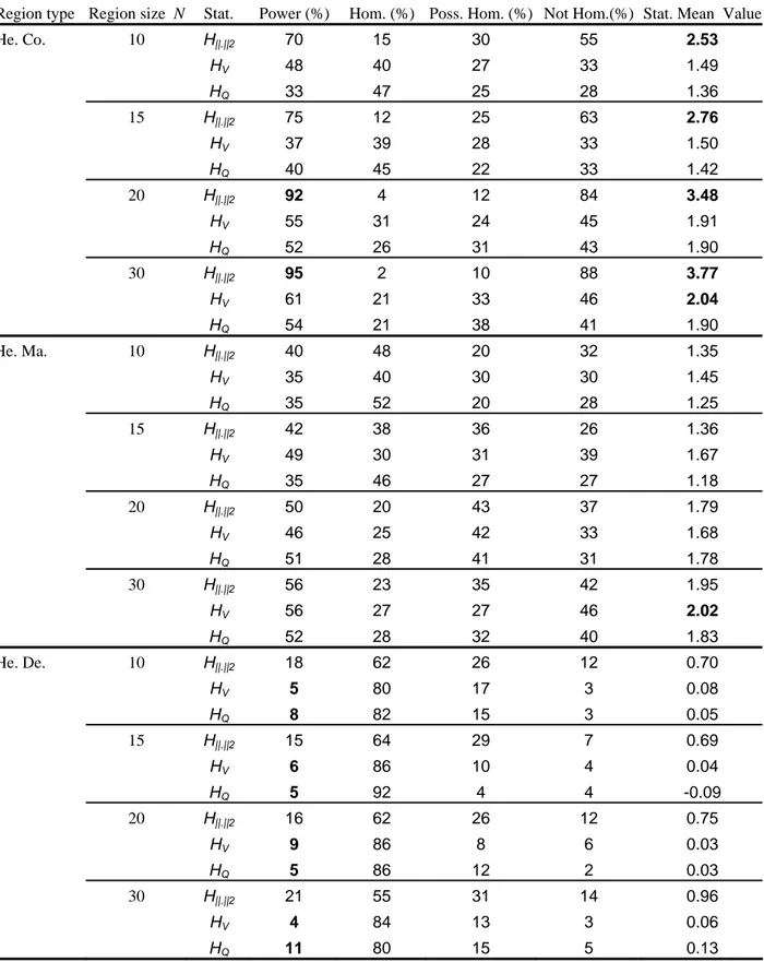
Table 4. Simulation results for homogeneity test when regions are 50% heterogeneous with n = 30
Region type Region size N Stat. Power (%) Hom. (%) Poss. Hom. (%) Not Hom.(%) Stat. Mean Value
He. Co. 10 H||.||2 70 15 30 55 2.53 HV 48 40 27 33 1.49 HQ 33 47 25 28 1.36 15 H||.||2 75 12 25 63 2.76 HV 37 39 28 33 1.50 HQ 40 45 22 33 1.42 20 H||.||2 92 4 12 84 3.48 HV 55 31 24 45 1.91 HQ 52 26 31 43 1.90 30 H||.||2 95 2 10 88 3.77 HV 61 21 33 46 2.04 HQ 54 21 38 41 1.90 He. Ma. 10 H||.||2 40 48 20 32 1.35 HV 35 40 30 30 1.45 HQ 35 52 20 28 1.25 15 H||.||2 42 38 36 26 1.36 HV 49 30 31 39 1.67 HQ 35 46 27 27 1.18 20 H||.||2 50 20 43 37 1.79 HV 46 25 42 33 1.68 HQ 51 28 41 31 1.78 30 H||.||2 56 23 35 42 1.95 HV 56 27 27 46 2.02 HQ 52 28 32 40 1.83 He. De. 10 H||.||2 18 62 26 12 0.70 HV 5 80 17 3 0.08 HQ 8 82 15 3 0.05 15 H||.||2 15 64 29 7 0.69 HV 6 86 10 4 0.04 HQ 5 92 4 4 -0.09 20 H||.||2 16 62 26 12 0.75 HV 9 86 8 6 0.03 HQ 5 86 12 2 0.03 30 H||.||2 21 55 31 14 0.96 HV 4 84 13 3 0.06 HQ 11 80 15 5 0.13
Stat.: Statistic. Hom.: Homogeneous. Poss. Hom.: Possibly Homogeneous. He. : Heterogeneous. Co.: Completely. Ma.: Marginally. De.: Dependence.
10 12 14 16 18 20 22 24 26 28 30 30 40 50 60 70 80 90 100 Po wer % N H||.|| 1 H||.|| 2 H||.|| F HV HQ
Figure 3.a. Test power for completely heterogeneous region with n = 30
In the second part of Table 4, results about marginal heterogeneity are presented. For a fixed N, the H mean values are approximately in the same order for all statistics. On the other hand, for each H statistic, the corresponding mean value increases with respect to N. Since all mean values range between 1 and 2, all procedures partially fail to indicate the right kind of heterogeneity. In terms of power, Figure 3.b shows that all the H homogeneity tests indicate the heterogeneity on the marginals with approximately the same power. Generally, powers increase with N in the range 35%-60%.
10 12 14 16 18 20 22 24 26 28 30 35 40 45 50 55 60 Po w e r % N H ||.|| 1 H ||.|| 2 H ||.|| F H V H Q
Figure 3.b. Test power for marginally heterogeneous region with n = 30
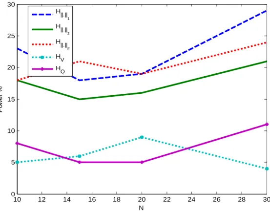
The simulation results, when the generated regions are heterogeneous on the dependence
parameter m, are presented in the last part of Table 4. The
2
.
H mean values increase slightly
with N whereas the mean values ofHV and HQ are almost constant. With mean values of H less
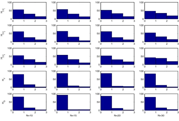
than 1, the bivariate and univariate approaches fail to indicate the right kind of heterogeneity. In Figure 3.c, we observe that, despite the low power of the bivariate tests, they perform clearly better than the univariate tests which fail to indicate any heterogeneity in that region. The power values concerning the univariate tests are around 5% which corresponds to the first kind error. Therefore, these results are not necessarily expected to be increasing with respect to N, since under the univariate tests, the regions are viewed as “homogeneous”. Figure 4 illustrates clearly the gain of the bivariate tests compared to the univariate tests, in terms of the occurrence rates.
Indeed, the first bar in each cell of Figure 4 is very high for the univariates in comparison with those of the bivariates. This means that the univariate tests lead to false conclusions concerning the heterogeneity on the dependence parameter.
10 12 14 16 18 20 22 24 26 28 30 0 5 10 15 20 25 30 Po w e r % N H ||.|| 1 H||.|| 2 H ||.|| F HV HQ
0 1 2 3 0 50 100 H||. ||1 0 1 2 3 0 50 100 0 1 2 3 0 50 100 0 1 2 3 0 50 100 0 1 2 3 0 50 100 H||. ||2 0 1 2 3 0 50 100 0 1 2 3 0 50 100 0 1 2 3 0 50 100 0 1 2 3 0 50 100 H|| .| |F 0 1 2 3 0 50 100 0 1 2 3 0 50 100 0 1 2 3 0 50 100 0 1 2 3 0 50 100 HV 0 1 2 3 0 50 100 0 1 2 3 0 50 100 0 1 2 3 0 50 100 0 1 2 3 0 50 100 HQ N=10 0 1 2 3 0 50 100 N=15 0 1 2 3 0 50 100 N=20 0 1 2 3 0 50 100 N=30
Figure 4. Rates of heterogeneity measure for dependence heterogeneous region with n = 30
From the previous remarks, it is important to make the following observation: When the
heterogeneity is on the two marginal parameters αV and αQ, the statistical test H has a lower power than in complete heterogeneity on all three parameters α αV, Q and m. However, powers in both above cases are higher than in heterogeneity on the only one dependence parameter m. This can be explained by the fact that the higher the heterogeneity in terms of the number of parameters to be varied, the higher the power will be.
The arguments previously developed for heterogeneous regions can also be presented when the regions are bimodal. Hence, the following discussion will be brief. The results of the homogeneity tests for the various 30% bimodal regions with site record length n=30 are
presented in Table 5 from which illustrations similar to Figures 3.a-3.c can be derived for powers. As shown in the fist part of Table 5, for the completely bimodal regions, the power of
the H. statistics ranges between 70% and 90%. These values are considerably higher than the
power of HV andHQ. The second part of Table 5 shows that, when the bimodality is on the
marginals, both univariate and bivariate tests have similar power values, generally less than 55%. The last part of Table 5 indicates that the bimodality on the dependence parameter m can not be detected by the univariate tests. On the other hand, bivariate tests identify the heterogeneity on dependence parameter m but with a low power. This power ranges between 15% and 30% for
30 n= .
The total record length of sites in the region has an effect on the performance of homogeneity tests. That is, the larger the total record length in the region, the higher the power will be. Indeed,
from Table 6, it can be seen that the power of
2
.
H is very high (96%) when
50, 46,...,10,14,...,50 i
n = where the total record length is 650. Both regions with 10,12,...,50
i
n = and ni =50, 48,...,10 correspond to moderate powers (69% and 78% respectively) where the total record length is 630. Finally, whenni =10,14,...,50, 46,...,10, the power is low (57%) as this corresponds to the shortest total record length of 610. In all these
variations of n, the power of
2
.
H is always higher than the power of both HV and H . Table 7 Q
shows that when site record lengths are high (n=60), except for the case of heterogeneity on the dependence parameter m, the power of all tests is very high and can reach 100% for
2
.
H . The
first kind error is then very close to the theoretical value of 5% for both univariate and bivariate tests. For dependence heterogeneous or dependence bimodal regions, the power of
2
.
considerably from 20% when n=30to 50% for n=60. On the other hand, for such regions, and
V Q
H H give always false results.
Finally, if a choice has to be made among the various norms, the authors suggest the adoption of
the . 2norm for both the homogeneity and discordancy tests. The reason for this choice is that,
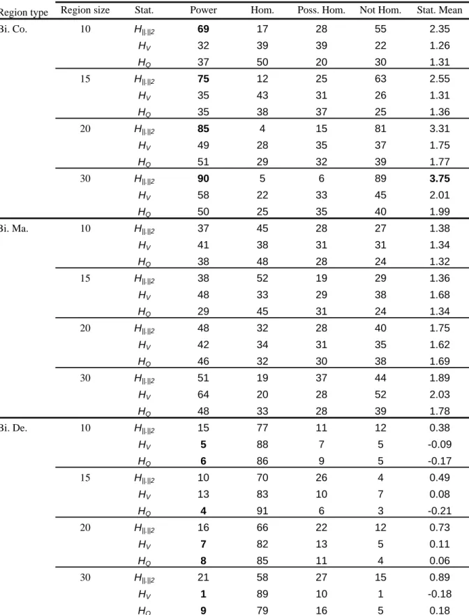
Table 5. Simulation results for homogeneity test when regions are 30% bimodal with n = 30
Region type Region size Stat. Power Hom. Poss. Hom. Not Hom. Stat. Mean
Bi. Co. 10 H||.||2 69 17 28 55 2.35 HV 32 39 39 22 1.26 HQ 37 50 20 30 1.31 15 H||.||2 75 12 25 63 2.55 HV 35 43 31 26 1.31 HQ 35 38 37 25 1.36 20 H||.||2 85 4 15 81 3.31 HV 49 28 35 37 1.75 HQ 51 29 32 39 1.77 30 H||.||2 90 5 6 89 3.75 HV 58 22 33 45 2.01 HQ 50 25 35 40 1.99 Bi. Ma. 10 H||.||2 37 45 28 27 1.38 HV 41 38 31 31 1.34 HQ 38 48 28 24 1.32 15 H||.||2 38 52 19 29 1.36 HV 48 33 29 38 1.68 HQ 29 45 31 24 1.34 20 H||.||2 48 32 28 40 1.75 HV 42 34 31 35 1.62 HQ 46 32 30 38 1.69 30 H||.||2 51 19 37 44 1.89 HV 64 20 28 52 2.03 HQ 48 33 28 39 1.78 Bi. De. 10 H||.||2 15 77 11 12 0.38 HV 5 88 7 5 -0.09 HQ 6 86 9 5 -0.17 15 H||.||2 10 70 26 4 0.49 HV 13 83 10 7 0.08 HQ 4 91 6 3 -0.21 20 H||.||2 16 66 22 12 0.73 HV 7 82 13 5 0.11 HQ 8 85 11 4 0.06 30 H||.||2 21 58 27 15 0.89 HV 1 89 10 1 -0.18 HQ 9 79 16 5 0.18
Stat.: Statistic. Hom.: Homogeneous. Poss. Hom.: Possibly Homogeneous. Bi.: Bimodal. Co.: Completely. Ma. : Marginally. De.: Dependence.
Table 6. Simulation results for homogeneity test when regions are 50% heterogeneous and variable n from site to site and N = 21
Region type Stat. Power (%) Hom. (%) Poss. Hom. (%) Not Hom. (%) Stat. Mean Value
He. Co. (a) H||.||2 69 1 21 61 2.33
HV 39 35 38 27 1.46 HQ 29 52 27 21 1.09 He. Co. (b) H||.||2 78 8 25 67 3.02 HV 48 3 30 40 1.98 HQ 43 47 17 36 1.63 He. Co. (c) H||.||2 57 22 33 45 2.28 HV 27 50 28 22 1.11 HQ 32 55 18 27 1.32 He. Co. (d) H||.||2 96 2 7 91 3.76 HV 70 14 31 55 2.26 HQ 63 21 28 51 1.99 (a) ni=10,12,…,50; (b) ni=50,48,…,10; (c) ni=10,14,…,50,46,…,10; (d)ni=50,46,…,10,14,…,50
Stat.: Statistic. Hom. : Homogeneous. Poss. Hom.: Possibly Homogeneous. He.: Heterogeneous. Co.: Completely.
Table 7. Simulation results for homogeneity test when n = 60 and N = 30 Region type Stat. Power (%) Hom. (%) Poss. Hom. (%) Not Hom. (%) Stat. Mean Value Hom. H||.||2 3 88 10 2 0.09 HV 7 84 14 2 0.02 HQ 6 87 9 4 0.14 He. Co. 50% H||.||2 100 0 0 100 7.19 HV 98 1 4 95 3.83 HQ 90 1 15 84 3.50 He. Ma.50% H||.||2 96 0 7 93 4.07 HV 96 2 6 92 3.95 HQ 94 2 8 90 3.68 He. De. 50% H||.||2 55 19 36 45 1.82 HV 6 86 12 2 -0.04 HQ 2 91 9 0 -0.09 Bi. Co. 30% H||.||2 100 0 0 100 7.22 HV 100 0 7 93 3.84 HQ 95 0 9 91 3.58 Bi. Ma. 30% H||.||2 97 0 6 94 4.06 HV 98 1 3 96 4.10 HQ 94 2 9 89 3.67 Bi. De. 30% H||.||2 53 28 31 41 1.79 HV 3 86 12 2 -0.02 HQ 10 81 15 4 0.11
Stat.: Statistic. Hom.: Homogeneous. Poss. Hom.: Possibly Homogeneous. He.: Heterogeneous. Bi.: Bimodal. Co.: Completely. Ma.: Marginally. De.: Dependence.
7. CONCLUSIONS
The approach presented in this paper is an extension to the multivariate context of the homogeneity test and discordancy statistic developed by Hosking and Wallis (1993) in a univariate setting. A bivariate version is applied on flood events described by their peaks and volumes, where the model is the Gumbel logistic with Gumbel marginal distributions. The approach is based on multivariate L-moments to define the statistics and on copula techniques for the modeling of the hydrological events. The multivariate tests have several advantages, including the control of the first kind error and the consideration of the correlation between variables. The proposed statistics are also easy to implement and to use. Simulations, based on the generation of bivariate samples from several kinds of regions, are used to illustrate the advantages of the homogeneity test and its usefulness in multivariate regional flood frequency analysis.
Results show that the Di 2 statistics give better indications about the discordant sites in a
heterogeneous region than both Di V, and Di Q, especially for sites where the whole structure of the
distribution is affected. Furthermore, the power of the proposed bivariate homogeneity tests
2
.
H
is very high, especially for regions with large sizes or large total record lengths. Both univariate
homogeneity tests HV and HQ lead to inferior performances compared to the bivariate test
2
.
H .
The difference is more significant when the heterogeneity is related to the dependence structure of the bivariate samples.
The performances of the proposed tests are influenced by various factors, such as the size of the
region N, the sites record lengths ni, the degree of regional heterogeneity and the kind of
heterogeneity (complete, marginal or on the dependence). For small regions or sites with short record lengths, these tests need to be improved in order to indicate heterogeneity that affects the dependence structure of the multivariate model. However, for these types of regions, univariate tests give false indications.
8. ACKNOWLEDGMENTS:
Financial support for this study was graciously provided by the Natural Sciences and Engineering Research Council (NSERC) of Canada, under funding to the Canada Research Chair on the estimation of hydrological variables. The authors wish to thank the Editor, Associate Editor and three anonymous reviewers whose comments helped improve the quality of the paper.
9. REFERENCES
Alila, Y. (1999) A hierarchical approach for the regionalization of precipitation annual maxima in Canada. J. Geophys. Res., 104, 31,645-31,655.
Alila, Y. (2000) Regional rainfall depth-duration-frequency equations for Canada. Water
Resour. Res., 36, 1767-1778.
Ashkar, F. (1980) Partial duration series models for flood analysis. PhD thesis, Ecole Polytechnique of Montreal, Montreal, Canada.
Ashkar, F.; El Jabi, N. and Issa, M. (1998) A bivariate analysis of the volume and duration of low-flow events. Stoch. Hydrol. Hydraul., 12, 97-116.
Bacchi, B.; Becciu, G. and Kottegoda, N. T. (1994) Bivariate exponential model applied to intensities and duration of extreme rainfall. J. Hydrol., 155, 225-236.
Burn, D. H. (1990) Evaluation of regional flood frequency analysis with a region of influence approach. Water Resour. Res., 26, 2257-2265.
Dalrymple, T. (1960) Flood frequency methods. United States Geological Survey Water-Supply
Paper, 1543 A, 11-51.
De Michele, C.; Salvadori, G.; Canossi, M.; Petaccia, A. and Rosso, R. (2005) Bivariate Statistical Approach to Check Adequacy of Dam Spillway. J. Hydrologic Engrg., 10, 50-57.
Durrans, S.R. and Tomic, S. (1996) Regionalization of low-flow frequency estimates: an Alabama case study. Water Resour. Bull., 32, 23-37.
Efron, B. and Tibshirani, R. (1994) An Introduction to the Bootstrap. Chapman & Hall/CRC.
El Adlouni, S.; Favre, A-C. and Bobée, B. (2004) Multivariate frequency analysis using Copulas.
DeMoSTAFI Conference “Dependence Modelling Statistical Theory and Application in
Finance and Insurance”. Québec, Canada 20-22 Mai 2004.
Fill, H. D. and Stedinger, J. R. (1995) Homogeneity tests based upon Gumbel distribution and a critical appraisal of Dalrymple's test. J. Hydrology, 166, 81-105.
Ghoudi, K.; Khoudraji, A. and Rivest, L-P. (1998) Propriétés statistiques des copules de valeurs extrêmes bidimensionnelles. Canad. J. Statist., 26, 87-197.
Goel, N. K.; Seth, S.M. and Chandra, S. (1998) Multivariate modeling of flood flows. ASCE J.
Hydraul. Eng., 124,146–155.
GREHYS (1996a) Presentation and review of some methods for regional flood frequency analysis. J. Hydrology, 186, 63-84.
GREHYS (1996b) Inter-comparison of regional flood frequency procedures for Canadian rivers.
J. Hydrology, 186, 85-103.
Gupta, V. K.; Duckstein, L. and Peebles, R. W. (1976) On the joint distribution of the largest flood and its time of occurrence. Water Resour. Res., 12, 295–304.
Horn, R. A. and Johnson, C. R. (1990) Matrix Analysis. Norms for Vectors and Matrices Ch. 5. Cambridge University Press. 575 pages.
Hosking, J. R. M. (1990). L-moments: analysis and estimation of distributions using linear combinations of order statistics. J. R. Stat. Soc. Ser. B, 52, 105-124.
Hosking, J. R. M. and Wallis, J. R. (1993) Some statistics useful in regional frequency analysis.
Water Resour. Res., 29, 271-282.
Hosking, J. R. M. and Wallis, J. R. (1997) Regional Frequency Analysis: An Approach Based on
L-Moments. Cambridge University Press. 240 pages.
Kim, T.; Valdés, J. B. and Yoo, C. (2003) Nonparametric Approach for Estimating Return Periods of Droughts in Arid Regions. J. Hydrologic Engrg., 8, 237-246.
Manly, B.F.J. (2005) Multivariate statistical methods, a primer, 3rd edition Chapman & Hall/CRC. 214 pages.
Nelsen, R. B. (1999) An introduction to copulas. Lecture Notes in Statistics, 139. Springer-Verlag, New York.236 pages.
Nguyen, V.-T.-V. and Pandey, G. (1996) A new approach to regional estimation of floods in Quebec. In: Delisle, C.E., Bouchard, M.A. (Eds.), Proceedings of the 49th Annual Conference of the CWRA, June 26–28, Quebec City. Collection Environnement de l'U. de M., 587–596.
Ondo, J-C.; Ouarda, T.B.M.J. and Bobée, B. (1997) Literature review of homogeneity and independent tests, in French, Research report INRS-Eau N° R-500. 78 pages.
Ouarda, T. B. M. J.; Haché, M.; Bruneau, P. and Bobée, B. (2000) Regional Flood Peak and Volume Estimation in Northern Canadian Basin. ASCE J. Cold. Reg. Engrg., 14, 176-191.