Abundance determination in massive stars: challenges for mixing processes

Département d’Astrophysique,

Université de Liège

Géophysique et Océanographie

Faculté des Sciences

Groupe d’AstroPhysique des

STAR Institute

Hautes Énergies (GAPHE)

Abundance determination in massive stars:

challenges for mixing processes

Thesis for the Degree of

Philosophiæ Doctor

Constantin Cazorla

Jury:

Dr. Yaël Nazé (supervisor)

University of Liège

Dr. Thierry Morel (co-supervisor)

University of Liège

Pr. Marc-Antoine Dupret

University of Liège

Dr. Sylvia Ekström

Observatory of Geneva

Dr. Yves Frémat

Royal Observatory of Belgium

Pr. Éric Gosset

University of Liège

Dr. Fabrice Martins

University of Montpellier

Pr. Gregor Rauw

University of Liège

v

Abstract:

Massive stars, the most luminous stars, are the true “cosmic engines” of

our Universe. They eject large quantity of material throughout their life,

which strongly influences their evolutionary path as well as their environment.

An important feature of massive stars is their high rotational velocities

that are either acquired at birth or due to the influence of a companion.

Rotation is believed to transport nitrogen-rich and carbon/oxygen-poor

material generated in the stellar core through the CNO cycle, to the surface.

A way to test the efficiency of rotational mixing is to study the chemical

composition at the surface of stars, in particular the fastest rotators.

The incentive for this study was the discovery, in the context of the

VLT-FLAMES Survey of Massive Stars, of fast rotators exhibiting an unenriched

nitrogen composition at their surface, contrary to predictions from single-star

evolutionary models including rotation. However, their multiplicity may

affect this conclusion, since both rotation and abundances can change as a

result of binary interactions. In this work, we combined, for the first time, a

detailed surface abundance analysis with a radial-velocity study to quantify

the importance of binary effects. This work was conducted for a sample of

40 bright, OB fast rotators in our Galaxy. Statistical tests and period-search

techniques revealed that ≥ 40% of our targets whose multiplicity status

can be probed, are binary or binary candidates. We derived the projected

rotational velocity of our targets and model atmosphere codes were then

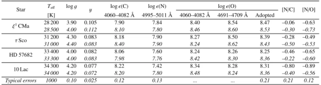
used to derive stellar parameters and surface abundances of all sample stars.

This abundance study revealed a correlation between the helium and nitrogen

abundances of our targets, which is predicted by the rotational mixing theory.

Finally, we compared our results to predictions of single-star evolutionary

models. We found that 10 – 20% of our 40 targets exhibit no enhancement of

the [N/O] abundance ratio, in line with results of the VLT-FLAMES Survey

of Massive Stars. The properties of only half of our sample are explained

by such models, and surprisingly we also uncovered a quite common large

abundance of helium at the surface of our targets. Modifying the diffusion

coefficient in single-star models and models of non-rotating mergers did

not reproduce simultaneously both the observed helium abundances and the

[N/O] abundance ratios. Binary models considering a mass-transfer episode

can, however, reproduce the [N/O] values of the majority of our targets and

even the helium abundances of some of the most helium-enriched targets,

but they cannot explain stars displaying little helium enrichment but high

vi

[N/O] values. In conclusion, we found that not every feature of massive stars

can be explained by models, suggesting that they lack a physical ingredient

and thus require further improvements.

The second part of this thesis aimed at improving our knowledge of the X-ray

emission of early B-type stars. We studied 11 such stars at high resolution

thanks to two X-ray facilities, XMM-Newton and Chandra, doubling the

number of B-stars analysed at high resolution. In many aspects, our study

confirmed previous ones: early B-stars display rather narrow and unshifted

lines arising from a warm (of typically 0.2 – 0.6 keV) plasma located at a few

stellar radii over the stellar surface. We also found that abundances derived in

the X-ray domain are in fair agreement with photospheric ones derived in the

optical domain. Furthermore, most early B-stars are moderately bright X-ray

emitters – though we also unexpectedly found that this X-ray emission varies,

on short and/or long timescales, for half of our sample. A few stars display

peculiar features: the presence of a very hot (1.6 – 4.4 keV) component and

strong variations. These features suggest that the recorded X-ray emission

may not be entirely linked to the B-stars, but could be contaminated by

emission from a companion or an interaction with it. Indeed, in one case,

HD 79351, a flare was detected, of a luminosity compatible with those from

PMS stars, and which could be associated to its companion. Finally, the

data used also led to the discovery of the second case of X-ray pulsations

associated to — Cephei activity.

Résumé :

Les étoiles massives, qui sont les étoiles les plus lumineuses, sont les véritables

“moteurs cosmiques” de notre Univers. Elles éjectent de grandes quantités

de matière au cours de leur vie, ce qui influence fortement leur évolution

ainsi que leur environnement. Une caractéristique importante de ces étoiles

massives est leur vitesse de rotation élevée qu’elles acquièrent à leur naissance

ou suite à l’influence d’un compagnon. Cette rotation est censée induire

un transport de la matière riche en azote et pauvre en carbone/oxygène,

créée au coeur des étoiles massives au travers du cycle CNO, à leur surface.

Une façon de tester l’efficacité d’un tel mélange rotationnel est d’étudier la

composition chimique à la surface d’étoiles, en particulier celles présentant

la rotation la plus rapide.

La motivation de cette étude était la découverte, dans le contexte du projet

VLT-FLAMES Survey of Massive Stars, de rotateurs rapides montrant une

composition chimique non-enrichie en azote à leur surface, contrairement

à ce qui est prédit par les modèles d’évolution d’étoiles isolées considérant

la rotation de ces étoiles. Cependant, leur multiplicité peut affecter cette

conclusion, du fait que la rotation et les abundances peuvent être modifiées

à la suite d’interactions au sein de systèmes binaires. Dans ce travail, nous

avons combiné, pour la première fois, une analyse détaillée des abondances de

surface avec une étude des vitesses radiales pour quantifier l’importance des

effets de binarité. Ce travail a été réalisé pour un échantillon de 40 rotateurs

rapides brillants, de type spectraux OB et faisant partie de notre Galaxie.

Des tests statistiques ainsi que des techniques de recherche de périodes ont

révélé que ≥ 40% de nos cibles dont la multiplicité a pu être déterminée

sont des binaires ou des candidats binaires. Nous avons déterminé la vitesse

de rotation projetée de nos cibles. Des codes de modèles d’atmosphère

ont ensuite été utilisés pour déterminer les paramètres stellaires ainsi que

les abondances de surface des étoiles de notre échantillon. L’étude des

abondances a révélé une correlation entre les abondances d’hélium et d’azote

de nos cibles, comme prédit par la théorie du mélange rotationnel. Enfin,

nous avons comparé nos résultats avec les prédictions de modèles d’évolution

d’étoiles isolées. Nous avons trouvé que 10 – 20% de nos 40 cibles ne

montre pas d’élévation du rapport d’abondance [N/O], en accord avec les

résultats du VLT-FLAMES Survey of Massive Stars. Seule la moitié des

étoiles de notre échantillon ont leur propriétés expliquées par ces modèles,

viii

et, étonnamment, une importante abondance d’hélium a fréquemment été

trouvée à la surface de nos cibles. La modification du coefficient de diffusion

dans les modèles d’étoiles isolées ainsi que les modèles résultant de la fusion

de deux étoiles n’ont pas permis de reproduire simultanément les abondances

d’hélium et les rapports d’abondance [N/O] observés. Les modèles d’étoiles

binaires considérant un épisode de transfert de masse peuvent, cependant,

reproduire les valeurs du rapport [N/O] de la majorité de nos cibles et même

les abondances d’hélium de certaines étoiles qui présentent le plus important

enrichissement en hélium, mais ils ne peuvent pas expliquer le fait que

des étoiles présentent un faible enrichissement en hélium mais des rapports

[N/O] élevés. En conclusion, nous avons trouvé que l’ensemble des propriétés

des étoiles massives ne peut pas être expliqué par les modèles d’évolution

actuels, ce qui suggère qu’un ingrédient physique nécessite d’y être intégré,

nécessitant donc un développement supplémentaire.

La seconde partie de cette thèse avait pour but d’améliorer notre connaissance

sur l’émission X d’étoiles de type spectral B précoces. Nous avons étudié 11

de ces étoiles grâce à deux télescopes (XMM-Newton et Chandra) permettant

l’acquisition de données de haute résolution, ce qui a permis de doubler le

nombre d’étoiles B étudiées à haute résolution. À bien des égards, notre étude

a confirmé plusieurs études antérieures: les étoiles B précoces présentent des

raies non décalées et plutôt étroites, qui sont créées par un plasma chaud (à

typiquement 0.2 – 0.6 keV) localisé à plusieurs rayons stellaires à partir de

la surface. Nous avons aussi trouvé que les abondances déterminées dans

le domaine des rayons X sont en bon accord avec celles déterminées pour

la photosphère dans le domaine visible. De plus, la plupart des étoiles B

précoces sont des émetteurs de rayons X modérément brillantes – bien que

nous ayons trouvé de manière inattendue une variation de cette émission

X sur de courtes et/ou longues périodes de temps pour la moitié de notre

échantillon. Certains objets montrent des propriétés particulières: la présence

d’une composante très chaude (de 1.6 – 4.4 keV) et de fortes variations de

l’émission X. Ces propriétés suggèrent que l’émission X observée peut ne pas

être entièrement liée à l’étoile B, mais peut être contaminée par de l’émission

par un compagnon ou une interaction avec celui-ci. En effet, dans le cas de

HD 79351, une éruption stellaire a été détectée, avec une luminosité en accord

avec celles des éruptions d’étoiles pré-séquence principale : le changement de

luminosité est donc peut-être lié à son compagnon. Finalement, les données

que nous avons utilisées ont aussi mené à la découverte d’un second cas de

pulsations X associées à une activité — Cephei.

List of Papers

Referred publications related to the thesis:

I Cazorla, C., Morel, T., Nazé, Y., Rauw, G., Semaan, T., Daflon, S.,

Oey, M. S., 2017a,

Chemical abundances of fast-rotating massive stars. I. Description of

the methods and individual results

A&A, 603, A56

II Cazorla, C., Nazé, Y., Morel, T., Georgy, G., Godart, M., Langer, N.,

2017b,

Chemical abundances of fast-rotating massive stars. II. Interpretation

and comparison with evolutionary models

A&A, accepted

III Cazorla, C. & Nazé, Y., 2017c,

B-stars seen at high resolution by XMM-Newton

A&A, submitted

Unreferred publications not related to the thesis:

I Proceedings following the IAU Symposium 307 (Geneva, 23rd – 27th June

2014): New windows on massive stars: asteroseismology, interferometry,

and spectropolarimetry,

Cazorla, C., Morel, T., Nazé, Y., Rauw, G., 2015,

Chemical abundances of fast-rotating OB stars,

G. Meynet, C. Georgy, J.H. Groh & Ph. Stee, eds., 307, 94

II Poster exhibiting results obtained in the X-ray domain with

XMM-Newton, during the X-ray Universe 2017 Symposium (Rome, 6th – 9th

June 2017)

Nazé, Y., Cazorla, C., Rauw, G., Morel, T., 2017,

A legacy survey of early B-stars using the RGS

xii

Referred publications not related to the thesis:

I Cazorla, C., Nazé, Y., Rauw, G., 2014,

Wind collisions in three massive stars of Cygnus OB2

A&A, 561, A92

II Nazé, Y., Rauw, G., Cazorla, C., 2017,

fi

Aqr is another “ Cas object

Contents

Abstract

v

List of Papers

xi

List of Abbreviations

xv

List of Tables

xix

List of Figures

xxi

1 Background and motivation

1

1.1 General context

. . . .

2

1.1.1 Massive stars

. . . .

2

1.1.2 Stellar rotation

. . . .

4

1.1.2.1 Stellar shape and critical velocities

. . . . .

6

1.1.2.2 Gravity darkening effect

. . . .

9

1.1.2.3 Transport of angular momentum and

chem-ical elements

. . . 16

1.1.3 Multiplicity

. . . 23

1.1.4 X-rays from massive stars

. . . 24

1.2 Thesis outline

. . . 27

1.2.1 Rationale of the study

. . . 27

2 Optical study

31

2.1 Derivation of abundances

. . . 32

2.1.1 Methods and tools

. . . 32

2.1.1.1 Projected rotational velocity

. . . 32

2.1.1.2 Turbulence broadening

. . . 33

2.1.1.3 Atmospheric parameters and He, CNO

abundances

. . . 34

2.1.2 Published paper

. . . 40

2.1.2.1 Complementary information

. . . 98

2.2 Comparison with evolutionary models

. . . 106

2.2.1 Stellar models

. . . 106

2.2.2 Published paper

. . . 113

2.2.2.1 Complementary information

. . . 137

3 X-ray study

141

3.1 Used X-ray facilities

. . . 142

xiv

Contents

3.2 Some X-ray properties of stars

. . . 144

3.3 Published paper

. . . 147

4 Conclusions and Perspectives

163

5 Acknowledgements

169

Bibliography

171

List of Abbreviations

ACIS Advanced CCD Imaging Spectrometer

ALI

Accelerated Lambda Iteration

ATHENA/X-IFU Advanced Telescope for High-ENergy

Astrophysics/X-ray Integral Field Unit

BONNSAI BONN Stellar Astrophysics Interface

CCD Charge-Coupled Device

CLÉS Code Liégeois d’Évolution Stellaire

CMFGEN CoMoving Frame GENeral

CPU Central Processing Unit

ELT

Extremely Large Telescope

EPIC European Photon Imaging Camera

ESA

European Space Agency

eV

Electron-Volt

EW

Equivalent Width

FASTWIND Fast Analysis of STellar atmospheres with WINDs

FIP

First Ionisation Potential

FLAMES Fibre Large Array Multi-Element Spectrograph

FWHM Full-Width at Half Maximum

GSF

Goldreich-Schubert-Fricke

HEG High Energy Grating

HETGS High Energy Transmission Grating Spectrometer

HMXB High Mass X-ray Binary

xvi

Contents

HRC High Resolution Camera

HRI

High Resolution Imager

HR

Hertzsprung-Russell

LBV Luminous Blue Variable

LETGS Low Energy Transmission Grating Spectrometer

LMC Large Magellanic Cloud

LOSP Liège Orbital Solution Package

MCWS Magnetically-Confined Wind Shock

MC

Magellanic Cloud

MEG Medium Energy Grating

MESA Modules for Experiments in Stellar Astrophysics

MiMeS Magnetism in Massive Stars

MOS Metal Oxide Semi-conductor

MS

Main Sequence

NASA National Aeronautics and Space Administration

NLTE Non-Local Thermodynamic Equilibrium

NS

Neutron Star

OM

Optical Monitor

PMS Pre-Main Sequence

PoWR Potsdam Wolf-Rayet

PSPC Position Sensitive Proportional Counters

RASS ROSAT All Sky Survey

Contents

xvii

RGA Reflection Grating Array

RGS Reflection Grating Spectrometer

RLOF Roche-Lobe Overflow

RV

Radial Velocity

SB1

Single-lined Spectroscopic Binary

SB2

Double-lined Spectroscopic Binary

sdO

Subdwarf O star

UV

UltraViolet

VLT

Very Large Telescope

WFC Wide Field Camera

WR

Wolf-Rayet

XMM-Newton X-ray Multi-Mirror Mission-Newton

XRT X-Ray-Telescope

List of Tables

1.1 Predicted Eddington factor for MS stars (for a core hydrogen

mass fraction of 0.30) at the middle of the MS phase and

the first critical velocity as a function of the initial stellar mass

9

1.2 Galactic fast-rotating stars whose surface CNO abundances

had been studied prior to our work

. . . 29

2.1 Differences in atmospheric parameters and He, CNO

abun-dances found for HD 163892 when the broadening of

DE-TAIL/SURFACE spectra is not only due to the stellar rotation

(and microturbulence), but also to macroturbulence

. . . 35

2.2 Changes in the atmospheric parameters and surface

abun-dances when HD 163892 is analysed with Kurucz models

using a helium abundance twice solar

. . . 100

2.3 Impact of the uncertainty in effective temperature on CNO

abundances

. . . 102

2.4 Tentative orbital solutions, presented for completeness,

ob-tained with the LOSP program for two stars of our sample

. 104

2.5 Information on the X-ray emission for our targets

. . . 105

2.6 Rotating single stellar models, starting from 2000

. . . 108

2.7 Comparison between the observed helium abundance and

[N/O] abundance ratios with predicted values by BONNSAI,

as a function of input parameters

. . . 138

3.1 List of our studied X-ray emitters

. . . 147

List of Figures

1.1 HR diagram

. . . .

3

1.2 Illustration of the energy transport processes at work in

solar-type and more massive stars

. . . .

3

1.3 CNO cycle

. . . .

4

1.4 Illustration of the projected rotational velocity

. . . .

6

1.5 Probability density of equatorial and projected rotational

velocities for 496 stars with spectral types O9.5 – B8

. . . .

6

1.6 Illustration of the stellar distorsion of a rotating star as a

function of the Ê ratio

. . . 10

1.7 Illustration of v

as a function of the stellar masses, for

different Z

. . . 11

1.8 Predicted v sin i as a function of log g

. . . 11

1.9 Derived v sin i as a function of the log g

for field and

cluster stars

. . . 12

1.10 Illustration of the variation in T

over the surface of a

rotating star as a function of ◊

. . . 13

1.11 Near-infrared intensity image of Altair

. . . 13

1.12 Illustration of the rotational broadening of a line profile.

Im-pact of the rotational velocity on line profiles. Line widths of

the He I 4471 line profile predicted for a B2-type spherical or

flattened star as a function of v sin i/v

. . . 14

1.13 Variation of the luminosity as a function of the Ê ratio for

several stellar masses

. . . 15

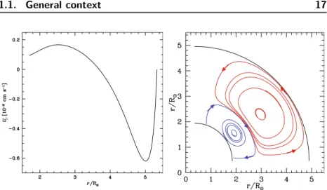
1.14 Illustration of the meridional circulation within a 20 M

rotating star with an initial rotational velocity of 300 km s

₁₇

1.15 Illustration of the differential rotation

. . . 19

1.16 Comparison of the diffusion coefficients in a 20 M

rotating

star with an initial rotational velocity of 300 km s

_{at the}

beginning of the MS phase

. . . 20

1.17 Surface nitrogen abundance at the middle and at the end of

the MS phase as a function of the initial stellar mass

. . . . 22

1.18 Schematic evolution of a massive close binary system

. . . . 25

1.19 Nitrogen abundance as a function of the projected rotational

velocity for stars with log g Ø 3.20 dex in extended regions

xxii

List of Figures

2.1 Illustration of the way the projected rotational velocity was

estimated, for HD 93521, with the He I 6678 line profile

. . 33

2.2 Illustration of the variation of the EW of some Si III line

profiles as a function of ›

. . . 35

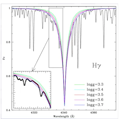
2.3 Illustration of the broadening of the wings of H“ with log g

. 39

2.4 Illustration of the curve of growth: evolution of the EW as a

function of the number of absorbing atoms

. . . 40

2.5 Predicted distribution of v sin i for MS massive stars

assum-ing the binary properties of Sana et al. (2012)

. . . 99

2.6 Illustration of the determination of v sin i and v

of HD

93521 thanks to spectral synthesis, using the He I 4921 line

100

2.7 Grid of synthetic spectra used to derive the atmospheric

parameters and helium abundance for the cooler stars

. . . . 101

2.9 Fourier periodogram derived from the RVs of HD 28446A.

Phase diagram of the RV values of HD 28446A folded with

a 3.37730 d period

. . . 103

2.10 Fourier periodiogram derived from the RVs of HD 41161.

Phase diagram of the RV values of HD 41161 folded on a

3.26594 days period

. . . 104

2.11 Difference between our parameter estimates and those found

by Martins et al. (2015a,b) as a function of the difference in

temperature

. . . 106

2.12 Difference between our parameter estimates and those found

by Martins et al. (2015a,b) as a function of the difference in

surface gravity

. . . 107

2.13 Difference between our [N/O] abundance ratio estimates and

those found by Martins et al. (2015a,b) as a function of the

difference in [N/C]

. . . 109

2.14 Histograms of the differences between our results and those

derived by Martins et al. (2015a,b), normalised by the errors

110

2.15 Predicted v sin i as a function of log g

by the Geneva and

Bonn models

. . . 111

2.16 Difference between the predicted [N/O] abundance ratios

by BONNSAI when first and second sets and first and third

sets of input parameters are used as a function of difference

1

Background and

motivation

The first chapter introduces massive stars, some of their properties, as well

as the rationale for this thesis.

2

1. Background and motivation

1.1

General context

1.1.1

Massive stars

Massive stars are stars whose mass is greater than 8 solar masses and with

spectral types O and early-B when on the main sequence. They are therefore

situated in the upper left part of the Hertzsprung-Russell (HR) diagram, as

shown in Fig.

1.1

. These massive stars are the true “cosmic engines” of our

Universe. These stars are the most luminous ones and are able to ionise the

interstellar medium. They eject large quantities of material in the interstellar

medium throughout their life (through a clumped stellar wind) following the

action of their strong ultraviolet (UV) radiation. Such winds modify their

evolutionary path, shape the interstellar medium, trigger or halt neighbouring

stellar formation, and largely contribute to the chemical enrichment of their

surroundings. Their mass-loss rates amount to ƒ 10

_M

§

yr

for O-type

star on the main-sequence (MS,

Martins et al. 2004

) with wind velocities of

several thousands km s

_{, and up to 10}

_M

§

yr

for short-lived luminous

blue variable (LBV) stages (

Vink & de Koter 2002

;

Smith et al. 2004

;

de

Koter 2006

;

Groh et al. 2009

). Massive stars finally explode in supernovae,

this phenomenon having a large impact on their surroundings. For all these

reasons, it is essential to get an in-depth comprehension of massive stars.

This work is aimed at modestly contributing to a better understanding of

these fascinating objects.

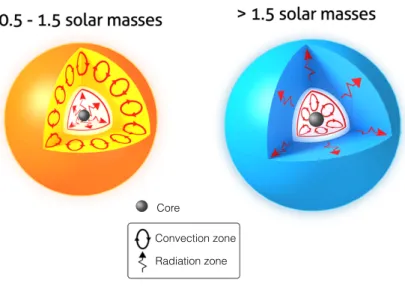
Massive stars have a different internal structure than that of solar-type stars,

as illustrated in Fig.

1.2

. Stars similar to the Sun have, from the core to the

surface, first a radiative zone and then a convective envelope. The situation

is opposite for massive stars as they have a convective zone near their core

and a radiative envelope. A thin convective zone due to opacity peaks linked

with iron and helium ionisations is also present in the outer layers of some

very luminous massive MS stars, but it contains a negligible amount of mass

(

Iglesias et al. 1992

;

Stothers & Chin 1993

;

Iglesias & Rogers 1996

;

Cantiello

et al. 2009

). Matter in the outer layers is therefore not mixed except if some

additional process takes place.

Massive stars burn their central hydrogen content through the CNO cycle

(Fig.

1.3

). Stars whose mass does not exceed ≥ 40 M

experience the

CNO-I cycle, which starts by converting atoms of

1.1. General context

3

Figure 1.1: HR diagram. OB stars are highlighted with the red rectangle. Source:

Astronomy magazine c .

Core

Convection zone Radiation zone

Figure 1.2: Illustration of the energy transport processes at work in solar-type

(left) and massive stars (right). Source: adapted from

http://www.sun.org/

images/heat-transfer-in-stars

4

1. Background and motivation

17

8

O

17

9

F

16

8

O

13

6

C

13

7

N

12

6

C

15

7

N

15

8

O

(p, )

14

7

N

(p, )

18

9

F

18

8

O

(p, )

19

9

F

(p, )

(p, )

(p, )

(p, )

I

II

III

IV

(p, )

(p, )

(p, )

Figure 1.3: CNO cycle. The part of the diagram highlighted in gray shows the

CN- and ON-cycles. Carbon and nitrogen, oxygen-17 and nitrogen, and oxygen-18

and nitrogen are the catalysts for the CN,

_{ON, and}

_{ON cycles, respectively.}

The different branches of the CNO cycle are indicated by the roman numbers.

The limiting reaction that follows is the source of an excess of nitrogen and

a depletion of carbon in the stellar core. This cycle is also called the CN

cycle because it does not involve a stable isotope of oxygen. Heavier stars go

even further by entering into the ON cycles (also called CNO-II & III cycles),

in which the atoms of

8

O are slowly destroyed to produce

N atoms. The

number of atoms of

6

C can be considered as constant in these cycles, but

it also leads to a nitrogen excess in the core.

1.1.2

Stellar rotation

Understandably, the first star that has been studied by astronomers is the

Sun. Thomas Harriot was probably the first European to notice the presence

of spots at the surface of the Sun, as demonstrated by drawings from 8th

December 1610 found in his notebook. Johannes Fabricius was the first to

observe the motion of sunspots on the solar surface and to publish these

1.1. General context

5

observations, in De Maculis in Sole Observatis, et Apparente earum cum

Sole Conversione Narratio, 1611. His findings were in disagreement with

the views of Christopher Scheiner, who proposed that the spots might be

small planets revolving around the Sun. Galileo Galilei confirmed in 1612

the discovery of Fabricius, by noticing a change in the size and shape of

sunspots as they move towards the solar equator, which is incompatible

with the view of Scheiner, and that proves that the Sun is rather a rotating

object. The Sun is not the only star to rotate, of course. In this context,

it is important to note the high rotational velocities of massive stars. They

are characterised by projected rotational velocities, v sin i (where v is the

stellar rotational velocity at the equator and i the angle between the line of

sight and the rotation axis; see Fig.

1.4

), typically a hundred times the Sun’s

value (Fig. 1.5). Such fast rotation can be acquired at birth, as a result

of their formation in molecular clouds under the action of gravity. The size

r

of these clouds is drastically reduced during the collapse (from typically

a few parsecs to a few solar radii), which implies a severe increase of their

angular velocity

according to the angular momentum conservation law

r

= constant – it has nevertheless to be noted that a significant amount

of angular momentum is lost during the stellar formation process though

interactions with the accretion disk. Fast rotation can also develop during

the stellar evolution when a star interacts with its companion (see Sect.

1.1.3

). The importance of rotation on the evolution of massive stars is now

considered to be comparable to that of stellar winds, influencing all aspects

of stellar evolution models (

Meynet & Maeder

,

2000

). The next subsections

briefly present these consequences.

6

1. Background and motivation

i

v

v sin i

i

v

v sin i

Figure 1.4: Illustration of the

pro-jected rotational velocity.

Source:

adapted from

https://en.wikipedia.

org/wiki/Stellar_rotation

B. Impact on the early chemical evolution

of galaxies 55

C. The carbon-enhanced metal-poor stars 58

D. The chemical anomalies in globular clusters 58

XIII. Conclusions 59

I. INTRODUCTION

It may be surprising that we emphasize the need of ac-counting for the effects of rotation in stellar evolution, since in practice all stars are rotating around their axis. However, it must be recalled that the so-called ‘‘standard theory’’ of stellar evolution generally ignores the effects of stellar rota-tion and treats the stars as nonrotating bodies, despite the fact that stars more massive than about 1:5M_!rotate fast on the average (Fig.1).

Recent progresses in astrophysical observations, particu-larly in high resolution spectroscopy and in asteroseismology, show many significant deviations from the standard models, for example, the many large nitrogen enrichments resulting from mixing in massive stars (Sec.VII). These observations show the need to also account for the various effects of rotation in stellar modeling. All model outputs are finally modified by the proper account of rotation: the stellar lumi-nosities and radii, the lifetimes, the chemical abundances at the surface, the helioseismology and asteroseismology re-sponses, the nature of supernova explosions, the amounts of nucleosynthetic products, the nature of the final remnants, etc.

For practical purposes, it is often convenient to distinguish four main groups of rotational effects in stellar physics.

(1) The equilibrium configuration of rotating stars: It results from the centrifugal force on the stellar equilibrium. The equipotentials are modified and, in particular, the shape of the stellar surface, which affects the surface Teff and

gravity distributions.

(2) The effects of rotation on mass loss or accretion: In fast-rotating stars, the isotropy of mass loss (or accretion when present) is destroyed and anisotropies appear and are effectively observed.

(3) The rotational mixing: The internal distortion induces circulation currents which transport the elements and angular momentum, while differential rotation may produce several instabilities which also contribute to the transport processes. (4) The interactions with magnetic field: The presence of an internal magnetic field may produce an internal coupling of rotation, leading to solid body rotation, while external fields produce some magnetic braking. A major uncertainty concerns the existence of a dynamo in radiative regions with differential rotation. We examine some properties of such a dynamo.

The above distinction is evidently a simplification since the various effects are related. For example, it is the modification of the internal equilibrium structure which drives the mixing. In turn, the mixing modifies the internal distribution of the elements and this also influences the equilibrium structure.

In this review, we focus on the rotational effects in the main sequence (MS) and post-MS phases, i.e., in the nuclear phases. The effects of rotation in star formation are also a most important chapter of astrophysics, but they would de-serve another specific review. We consider here the case of single stars, the many effects of rotation in relation with tidal interactions in binaries are also beyond the scope of this review. Most of the effects discussed here in the case of single stars evidently have their counterparts in binaries, however their modeling is still in its infancy.

Recent reviews on the observational and theoretical as-pects of stellar rotation are given in IAU symposium 215 (Maeder and Eenens, 2004) and the theoretical aspects have recently been extensively reviewed (Maeder, 2009).

II. THE MECHANICAL AND THERMAL EQUILIBRIUM OF ROTATING STARS

The equilibrium and stability configurations of rotating stars were reviewed long ago (Lebovitz, 1967). In practice, except for stars with little internal density contrast, such as white dwarfs or neutron stars, the approximation of the Roche model is acceptable. It assumes that the effective gravity results from the matter centrally condensed, in addition to the effect of the centrifugal force. For all stellar masses, the rotational energy of the Roche model represents at most about 1% of the absolute value of the potential energy.

The properties of rotating stars depend on the distribution of the angular velocity !_{ðrÞ inside the stars. The simplest} case is that of solid body rotation, i.e., !_{¼ const, while more} elaborate models include differential rotation.

A. The mechanical equilibrium for uniform rotation

We first consider the case of a constant angular velocity ! in the Roche model in hydrostatic equilibrium. The gradient of pressure P is given by 1 %rP ¼ % ~r" þ~ 1 2! 2_{rðr sin#Þ}~ 2_{; (1)}

% is the local density, " is the gravitational potential, which is unmodified by rotation in the Roche approximation and which gives the gravitational acceleration ~g¼ % ~r" ¼ %ðGMr=r2Þ~r=r, r being the distance to the center. The

FIG. 1. Probability density by km s%1of rotation velocities for

496 stars with types O9.5 to B8, i.e., masses between about 3M_!

and 20M_!. FromHuang and Gies, 2006a.

26 Andre´ Maeder and Georges Meynet: Rotating massive stars: From first stars to . . .

Rev. Mod. Phys., Vol. 84, No. 1, January–March 2012

Figure 1.5: Probability density of

rota-tional velocities for 496 stars with

spec-tral types O9.5–B8 (

Maeder & Meynet

2012

, with data from

Huang & Gies

2006

). For comparison, the Sun’s

rota-tional velocity is ≥ 2 km s

_.

1.1.2.1

Stellar shape and critical velocities

In the Roche approximation, in which the mass inside an isobar can be

considered as point-like, the total potential  is the sum of the gravitational

„

and the centrifugal ‰ potentials:

Â

(r, ◊) = ≠

GM

r

¸ ˚˙ ˝

≠

1

₂

r

sin

(◊)

¸

˚˙

˝

,

where r is the distance to the stellar centre, ◊ the colatitude, M

the mass

inside the radius r, and

is the angular velocity. The stellar surface is an

equipotential Â(r, ◊) = constant.

At the pole, r = R

, ◊=0, and one can write

Â

(R

,

0) = ≠

GM

R

1.1. General context

7

to the constant of the equipotential at the stellar surface. Thus, one has

GM

R

=

GM

r

+

1

2

r

sin

(◊)

(1.1)

Because of rotation, the effective gravity is thus modified:

˛g

= ˛g

+ ˛g

.

In spherical coordinates, the centrifugal and gravitational acceleration can

be expressed as

˛g

=

r

sin(◊)[sin(◊)˛e

+ cos(◊)˛e

];

˛g

= ≠

GM

r

e

˛

,

so that the effective gravity becomes

˛g

=

3

≠

GM

_r

+

r

sin

(◊)

4

˛

e

+

r

sin(◊) cos(◊)˛e

,

the modulus of ˛g

being

g

( , ◊) =

Û3

≠

GM

_r

+

r

sin

(◊)

4

+ (

_r

_{sin(◊) cos(◊))}

_(1.2)

One can define the critical, or break-up, angular velocity

, which is

reached when the modulus of the centrifugal acceleration ˛g

becomes

equal to the modulus of the gravitational acceleration ˛g

at the equator.

In this case, g

= 0 at the equator (for which ◊ = fi/2), so from Eq.

1.2

one obtains

2

crit

=

_R

GM

E,crit

(1.3)

where R

is the equatorial radius at critical velocity. Evaluating the Eq.

1.1

at the equator and introducing the expression of the critical angular

velocity leads to

R

R

=

3

2

.

(1.4)

This means that, at critical velocity, the equatorial radius is 1.5 times larger

than the polar one. The stellar shape for different angular velocities is

8

1. Background and motivation

illustrated in Fig.

1.6

. The stellar distorsion was investigated in some

interferometric studies, through the estimation of the R

/R

ratio. For

example, for the fast-rotating star Achernar (– Eri; B6Vpe,

Levenhagen &

Leister 2006

; v sin i ƒ 207 km s

_,

_{Yudin 2001}

_{), the measurements yield}

R

/R

≥ 1.4 – 1.5 (

Carciofi et al.

,

2008

), in agreement with the Roche

model with Ê = /

= 0.992.

One can now define with Eqs.

1.3

and

1.4

the first critical velocity:

v

=

R

=

GM

R

=

2

3

GM

R

.

(1.5)

This relation is valid under the Roche approximation (thus for solid body

rotation). Figure

1.7

illustrates the variation of v

as a function of the

initial stellar mass, for different metallicities.

Rotation is, however, not the only important physical ingredient. The

radiation pressure also plays a significant role inside massive stars by

coun-terbalancing the gravity. In this context, it can be shown that the validity

domain of Eq.

1.5

is limited to

<

0.639, where

is the local

Eddington factor at the surface of a rotating star. It typically describes the

anisotropy of a radiation field, and is defined by

Edd

( , ◊) =

Ÿ

( , ◊)L(P )

4ficGM

1

1 ≠

2fiG¯flM

2 ,

(1.6)

where Ÿ( , ◊) is the electron scattering opacity, c the celerity, and ¯fl

the

average stellar density. The first critical velocity does not depend on the

Eddington factor. This is due to the fact that as rotation increases, the

effective gravity at the equator decreases, thus, thanks to the von Zeipel

theorem, its effective temperature at the equator decreases accordingly,

keeping the radiation pressure negligible. However, the above expression

of the first critical velocity is no longer valid for stars with high radiation

pressure. For

>

0.639, one defines the second critical velocity as:

v

=

3

2

R

GM

R

E

(Ê)

_V

1 ≠

_(Ê)

.

with V

(Ê) = V (Ê)/#4/(3fiR

P,crit

)$, where V (Ê) is the total stellar volume.

The critical velocity decreases as

increases, so that a star with intense

radiation can rotate at its break-up velocity even if its rotational velocity is

low. Table

1.1

provides the Eddington factor for stars at the middle of the

1.1. General context

9

Table 1.1: Predicted Eddington factor for MS stars (for a core hydrogen mass

fraction X

of 0.30) at the middle of the MS phase (

) and the first critical

velocity v

as a function of the initial stellar mass. Source:

Maeder

(

2009b

).

Initial M

v

[M

]

[km s

]

120

0.544

711

85

0.436

646

60

0.343

623

40

0.239

586

25

0.136

536

20

0.098

513

15

0.060

487

12

0.039

466

9

0.021

439

MS phase, as well as the first critical velocity v

, as a function of the

initial stellar mass.

Evolution of the rotational velocity. Single-star models predict a

de-crease of the rotational velocity of a rotating star during its MS evolution,

as shown in Fig.

1.8

(see an example of observations in Fig.

1.9

). This is

due to the loss of angular momentum by stellar winds and the increase of

the radius during the stellar evolution. Note, however, that the predicted

rotational velocity in the models of

Brott et al.

(

2011

) for stellar masses

M

. 20 M

does not drastically change during the MS phase. This is due to

a competition of two effects: the increase of the rotational velocity thanks to

the transport of angular momentum to the surface, and the decrease of the

rotational velocity due to envelope expansion. This different behaviour in the

evolution of the stellar rotational velocity, compared to the Geneva models,

comes from the very different treatment of rotation, as the Geneva models

consider a less strong coupling between the stellar core and the envelope,

so that the spin-down by stellar winds is more effective (see Sect.

2.2.1

for

further comparisons between these two types of models).

1.1.2.2

Gravity darkening effect

The stellar deformation due to rotation induces a higher effective gravity

and a larger temperature at the stellar poles, hence a higher radiative flux

10

1. Background and motivation

2.1 Equilibrium Configurations

23

Fig. 2.2 The shape R(

ϑ) of a rotating star in one quadrant. A 20 M star with Z = 0.02 on the

ZAMS is considered with various ratios

ω = Ω/Ω

crit

of the angular velocity to the critical value

at the surface. One barely notices the small decrease of the polar radii for higher rotation velocities

(cf. Fig. 2.7). Courtesy of S. Ekstr¨om

Fig. 2.3 The variation of the ratio R

_e

/R

p

of the equatorial to the polar radius as a function of the

rotation parameter

ω in the Roche model

g

eff

=

_R

GM

₂

(

ϑ

)

+

Ω

2

_R(

_ϑ

_{) sin}

2

_ϑ

_e

r

+

Ω

2

R(

ϑ

) sin

ϑ

cos

ϑ

e

ϑ

.

(2.11)

The gravity vector is not parallel to the vector radius as shown in Fig. 2.1. The

modulus g

_eff

=

_|g

eff

| of the effective gravity is

Figure 1.6: The centrifugal forces triggered by rotation affect the stellar shape,

since their effect is to increase the equatorial radius, while slightly decreasing the

polar one (e.g.,

Collins 1963

;

Domiciano de Souza et al. 2003

). Illustration of the

distorsion of a rotating star of 20 M

on the zero age main sequence (ZAMS),

with Z = 0.020, as a function of the /

ratio. Source:

Maeder

(

2009b

).

(gravity darkening effect; Fig.

1.10

). A confirmation of this effect is given

by the observation of Altair, whose projected rotational velocity is ≥ 240

km s

_{and for which the ratio between its polar and equatorial effective}

temperatures is 1.23 – 1.27 (Fig.

1.11

,

Monnier et al. 2007

). Equation

1.2

shows that the effective gravity varies over the stellar surface. Since the

von Zeipel theorem provides a relation between the radiative flux (hence the

effective temperature) and the effective gravity, the effective temperature

will follow

T

( , ◊) =

3

_L

4fi‡GM

4

(g

)

_,

(1.7)

with

M

= M

3

1 ≠

_2fiG¯fl

4

,

where ‡ is the Stefan-Boltzmann constant. Note that another formulation

has been proposed by

Espinosa Lara & Rieutord

(

2011

), which implies a less

1.1. General context

11

S. Ekström et al.: Origin of Be stars

473

Fig. 10. Relation between /

and

=

/

obtained in the

frame of the Roche model. The continuous line is obtained assuming

R

/

R

= 1 (see text and Eqs. (9) and (11)). The dot-dashed lines

show the relations for the Z = 0.020 models with 1 and 60 M using

Eq. (8). The dotted line is the line of slope 1.

Fig. 11. Variations in the critical equatorial velocity on the ZAMS as a

function of the initial mass, for various metallicities.

3.3. Relations between /

_crit

and /

_crit

The relations between /

crit

and /

crit

obtained in the frame

of the Roche model (see Eq. (11)) for the 1 and 60 M stellar

models at Z = 0.02 are shown in Fig. 10. In case we suppose that

the polar radius remains constant (R

p,crit

/

R

p

= 1), then Eq. (9)

can be used and one obtains a unique relation between /

crit

and /

crit

, independent of the mass, metallicity, and

evolution-ary stage considered (continuous line). One sees that the values

of /

crit

are lower than that of /

crit

by at most ⇠25%. At the

two extremes, the ratios are of course equal.

3.4. Velocities on the ZAMS:

crit

,

Table 1 gives the angular velocity, the period, the polar radius,

and the equatorial velocity at the critical limit on the ZAMS for

the various models. Let us note that, for obtaining the value of

crit

or of whatever quantities at the critical limit, it is

neces-sary to compute models at the critical limit. Here we have

com-puted models very near, but not exactly at, the critical limit,

since at that point numerical singularities are encountered. As

explained in Sect. 2.2, using Eq. (9) we could have estimated

Table 1. Angular velocity, rotational period, polar radius, and equatorial

velocity at the critical limit on the ZAMS (solid body rotation).

M

Z

P

R

M

s

_h

_R

_{km s}

1

0

4.9E 04

3.6

0.8

400

1

10

_{4.9E 04}

_3.6

_0.8

₄₀₀

1

0.002

4.6E 04

3.8

0.8

390

1

0.020

4.6E 04

3.8

0.8

395

3

0

5.3E 04

3.3

1.1

595

3

10

_{5.1E 04}

_3.4

_1.1

₅₈₅

3

0.002

3.4E 04

5.1

1.4

515

3

0.020

2.2E 04

8.1

2.0

440

9

0

6.5E 04

2.7

1.4

920

9

10

_{3.5E 04}

_4.9

_2.0

₇₅₀

9

0.002

2.2E 04

8.1

2.8

635

9

0.020

1.5E 04

11.7

3.6

560

20

0

7.3E 04

2.4

1.6

1245

20

10

_{2.5E 04}

_7.0

_3.3

₈₇₀

20

0.002

1.6E 04

11.1

4.6

745

20

0.020

1.2E 04

15.2

5.6

670

60

0

4.6E 04

3.8

3.2

1540

60

10

_{1.7E 04}

_10.6

_6.4

₁₀₉₅

60

0.002

1.0E 04

16.9

8.7

935

60

0.020

7.0E 05

24.9

11.3

820

Fig. 12. Variations in the surface equatorial velocity on the ZAMS as a

function of initial rotation rate

=

/

for various metallicities and

masses. The coding for Z is the same as in Fig. 11.

crit

from whatever model was computed with a lower initial

ve-locity. Doing this for the whole range of initial masses,

metallic-ities and velocmetallic-ities, we would have obtained values within 10%

of those shown in Table 1. For the models between 3 and 20 M ,

the error would always be inferior to 3.5% because in this mass

range, R

p

( )/R

p

(0) remains very near 1 (see Fig. 2) and Eq. (9)

is a good approximation of Eq. (8). For the 1 and 60 M , the

er-rors would be larger, amounting to a maximum of 9.3 and 6.7%

respectively, showing the need to use instead Eq. (8) if

1.

In general the error decreases drastically when

increases, so

to obtain the values given in Table 1, we have used our faster

rotating model, deriving the value of

crit

(using Eq. (9)) with

an error less than 0.001%. The critical period, P

crit

is then

sim-ply given by P

crit

= 2⇡/

crit

. The polar radius is obtained

Figure 1.7: Illustration of the first critical velocity as a function of the initial stellar

mass, for different metallicities. Source:

Ekström et al.

(

2008b

).

log g [dex]3.6 3.4 3.2 3 3.8 4 4.2 v sin i [km s − 1] 100 150 200 250 300 350 400 M/M⊙= 15, vZAMS= 400 km s−1 M/M⊙= 20, vZAMS= 421 km s−1 M/M⊙= 25, vZAMS= 441 km s−1 M/M⊙= 32, vZAMS= 614 km s−1 M/M⊙= 40, vZAMS= 647 km s−1 M/M⊙= 60, vZAMS= 714 km s−1 log g [dex]3.6 3.4 3.2 3 3.8 4 4.2 M/M⊙= 15, vZAMS= 379 km s−1 M/M⊙= 20, vZAMS= 376 km s−1 M/M⊙= 25, vZAMS= 374 km s−1 M/M⊙= 30, vZAMS= 372 km s−1 M/M⊙= 40, vZAMS= 367 km s−1 M/M⊙= 60, vZAMS= 361 km s−1

Figure 1.8: Predicted projected rotational velocity as a function of the surface

gravity by

Georgy et al.

(

2013a

) and private comm. with Dr Georgy (left) and

Brott et al.

(

2011

, right). We assume i = 70

_{as fast rotators are preferentially}

12

1. Background and motivation

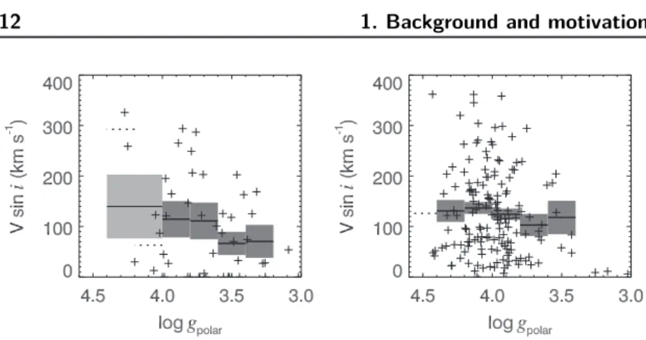
610

HUANG, GIES, & McSWAIN

Vol. 722

Figure 5. Scatter plots of V sin i as a function of log g

for the field (left column) and cluster samples (right column) and for three mass ranges: 2 < M/M

<

4 (top), 4

M/M

<

8 (middle), and M/M

8 (bottom). The solid horizontal lines indicate the mean V sin i of each bin containing six or more stars, while

dotted lines indicate the same for the bins containing fewer. Shaded areas illustrate the standard deviation of the mean for each bin.

matched pairs have similar mean V sin i (within one standard

deviation) except for one set with 3.6 < log g

<

3.8 in the

mid-mass subgroup. Note, however, that the number of field B

stars in the high-mass group (>8 M

) is small (a total of only

46 field B stars), and a larger sample would help establish the

details of the spin-down for this group. These results are very

similar to our previous findings (Huang & Gies

2008

), which

were based on a smaller sample of field stars. Thus, since the

spin-down trends appear to be similar in the field and cluster

stars and since the field stars tend to be more evolved (lower

log g

), we again conclude that the lower rotation rates of

the field stars are primarily the result of evolutionary spin-down

changes.

In contrast to our results, Wolff et al. (

2007

) did not detect a

significant evolutionary change in stellar rotation among their

sample of stars, and they concluded that differences in initial

conditions and mass densities of star-forming regions are key

to explaining the differences in rotational properties. Wolff

et al. (

2007

) compared rotational properties of B0–B3 stars

(corresponding to an approximate mass range of 6–12 M

) in

young and old clusters and associations in both low-density (ρ <

1 M

pc

_{) and high-density (ρ > 1 M}

⊙

pc

) environments.

They found that a small spin-down was evident when comparing

the cumulative distribution functions of V sin i for young and

old dense clusters (see their Figure 3). This relatively small

spin-down rate probably results in part because their sample

consists mainly of more massive B stars and because the

spin-down rates may be slower (as a function of log g

) among

massive B stars (see Figure

5

). Furthermore, some of the

spin-down trend may be lost when samples are binned according to

cluster age. The timescale of interest for evolutionary changes

is the MS lifetime, which depends sensitively on stellar mass,

τ

∝ M

. According to Schaller et al. (

1992

), a 6 M

star

has τ

= 63 Myr while a 12 M

star has τ

= 16 Myr. Thus,

while the young age group of cluster stars (1–6 Myr) considered

by Wolff et al. consists of mainly unevolved stars, the group of

older cluster stars (11–16 Myr) probably includes some evolved

massive stars (69%–100% τ

for M = 12 M

) and many

unevolved, lower mass stars (17%–25% τ

for M = 6 M

).

Thus, depending on the mass distribution of stars, the rotational

properties of the older group may show little or no evidence of

evolutionary spin-down because of the mixture of evolutionary

states represented within the sample.

Wolff et al. (

2007

) found much larger differences in the

rotational properties between stars in high and low-density

environments. By their criterion, all the cluster stars that we

Figure 1.9: Projected rotational velocity as a function of the polar surface gravity

for field (left) and cluster (right) stars with masses in the range 8ÆM.20 M

(plus signs). Solid horizontal lines represent the mean v sin i of each bin having

six or more stars, while dotted lines show the mean value for the bins containing

fewer stars. Shaded rectangles illustrate the standard deviation of the mean v sin i

for each bin. Source:

Huang et al.

(

2010

).

steep variation in T

.

One can also interpret the difference in flux (thus in effective temperature)

along the stellar surface as a consequence of the variation in the distance

between equipotentials. Several consequences of the gravity darkening effect

induced by rotation are worth mentioning.

Impact on the line widths. Rotation significantly modifies the emergent

spectrum of a rotating star as the Doppler effect broadens the spectral lines

(Figs.

1.12a

and

1.12b

). The gravity darkening effect induces a decrease

in the continuum emission of the equatorial regions, leading to smaller line

widths than in an uniform model. The line width even becomes insensitive

to rotation for very fast rotators, suggesting that the observational estimate

of their v sin i may systematically be underestimated (Fig.

1.12c

).

Impact on the luminosity. The flattening of a rotating star is also the

cause of a decrease in its surface averaged temperature, hence its luminosity.

An illustration of this effect is shown in Fig.

1.13

. The position in a

HR diagram of a rotating star is thus affected since the derived effective

temperature and luminosity depend on the angle of view under which the

star is seen.

1.1. General context

13

74

4 The Energy Conservation and Radiative Equilibrium in Rotating Stars

Fig. 4.1 Illustration of the von Zeipel theorem. The local T

eff

as a function of the colatitude

ϑ

for

models of 20 M on the ZAMS with various ratios

Ω

/

Ω

crit

of the angular velocity to the critical

value. The stellar shape is shown in Fig. 2.2. Courtesy G. Meynet

4.2.3 Interferometric Observations of Stellar Distortion

and Gravity Darkening

Interferometric observations by Domiciano de Souza et al. [164] of the Be star

Achernar (

α

Eri) with the VLTI indicate a ratio R

e

/R

p

1.5. After various claims,

a recent analysis of the data by Carciofi et al. [94] confirms that the observations

well agree with a rigidly rotating star at

_ω

= 0.992 in the Roche model, provided it

is surrounded by a small disk.

VLTI observations [165] of the fast rotating star Altair (M

1.8 M , A7IV-V)

confirm a gravity darkening as predicted by the von Zeipel theorem. A successful

fitting of the Roche model with a surface temperature following the von Zeipel

gravity darkening law is also reported by Peterson et al. [465] for Altair, which

rotates at 90% of its break-up angular velocity; this result is further confirmed [466].

The basic picture of gravity darkening is also supported by Monnier et al. [427],

but instead of an exponent 0.25 as in (4.23), an exponent 0.19 is favored. Also,

they notice an equatorial darkening stronger than predicted, which might result

from faster equatorial rotation, of differences due to convection or opacity

ef-fects, etc. Let us note that an exponent as small as 0.08 is found by van Belle

et al. [588] in the case of Alderamin (

α

Cep, type A7IV-V), which rotates at

83% of its break-up velocity. At this stage, we conclude that the possible

devia-tions from von Zeipel theorem is a subject of further theoretical and observational

investigations.

Figure 1.10: Illustration of the variation in effective temperature over the surface

of a rotating star of 20 M

on the ZAMS, with Z = 0.020, as a function of the

colatitude. Different Ê ratios are considered. Source:

Maeder

(

2009b

).