Improving configuration and planning optimization : towards a two tasks approach

HAL Id: hal-01847753

https://hal.archives-ouvertes.fr/hal-01847753

Submitted on 8 Nov 2018

HAL is a multi-disciplinary open access

archive for the deposit and dissemination of

sci-entific research documents, whether they are

pub-lished or not. The documents may come from

teaching and research institutions in France or

abroad, or from public or private research centers.

L’archive ouverte pluridisciplinaire HAL, est

destinée au dépôt et à la diffusion de documents

scientifiques de niveau recherche, publiés ou non,

émanant des établissements d’enseignement et de

recherche français ou étrangers, des laboratoires

publics ou privés.

Improving configuration and planning optimization :

towards a two tasks approach

Paul Pitiot, Michel Aldanondo, Élise Vareilles, Thierry Coudert, Paul Gaborit

To cite this version:

Paul Pitiot, Michel Aldanondo, Élise Vareilles, Thierry Coudert, Paul Gaborit. Improving

configu-ration and planning optimization : towards a two tasks approach. 15th International Configuconfigu-ration

Workshop, Aug 2013, Vienna, Austria. pp.43-50. �hal-01847753�

Abstract

This paper deals with mass customization and the association of the product configuration task with the planning of its production process while trying to minimize cost and cycle time. Our research aims at producing methods and constraint based tools to support this kind of difficult and constrained prob-lem. In some previous works, we have considered an approach that combines interactivity and optimiza-tion issues and propose a new specific optimizaoptimiza-tion algorithm, CFB-EA (for constraint filtering based evolutionary algorithm). This article concerns an improvement of the optimization step for large prob-lems. Previous experiments have highlighted that CFB-EA is able to find quickly a good approxima-tion of the Pareto Front. This led us to propose to split the optimization step in two sub-steps. First, a “rough” approximation of the Pareto Front is quickly searched and proposed to the user. Then the user in-dicates the area of the Pareto Front that he is inter-ested in. The problem is filtered in order to restrain the solution space and a second optimization step is done only on the focused area. The goal of the arti-cle is to compare thanks to various experimentations the classical single step optimization with the two sub-steps proposed approach.

1 Introduction

This article is about the concurrent optimization of product configuration and production planning. Each problem is considered as a constraint satisfaction problem (CSP) and these two CSP problems are also linked with some con-straints. In a previous paper [Pitiot et al., 2013], we have shown that this allows to consider a two-step process: (i) interactive configuration and planning, where non-negotiable user requirements (product requirements and production process requirements) are first processed thanks to constraint filtering and reduce the solution space (ii) op-timization of configuration and planning, where negotiable

requirements are then used to support the optimization of both product and production process.

Given this problem, product performance, process cycle time and process plus product cost can be optimized, we therefore deal with a multi-criteria problem and our goal is to propose to the user solutions belonging to the Pareto front. For simplicity we only consider cycle time and total cost (product cost plus process cost), consequently the two-step process can be illustrated as shown in figure 1.

Figure 1 - Two-step process

Some experimental studies, reported last year [Pitiot et al., 2012], discusses optimization performance according to problem characteristics (mainly size and constraint level). That last paper proposes to divide the step 2 (Pareto front computation) in two tasks, particularly in the case of large problems: (i) a first rough computation that permit to have a global idea of possible compromises (ii) a second computa-tion on a restricted area that is selected by the user. The goal of this article is to present experimental results that show that this idea allows to significantly reducing optimization duration while improving optimization quality.

In this introduction, we clarify with a very simple example what we mean by concurrent configuration and planning problem and relevant optimization needs. Then the second section formalizes the optimization problem, presents the optimization algorithm and describes the experimental study. The third section is dedicated to various experimenta-tions.

Improving configuration and planning optimization:

Towards a two tasks approach

Paul Pitiot

, Michel Aldanondo

, Elise Vareilles

, Thierry Coudert

, Paul Gaborit

University Toulouse – Mines Albi, France

2

3IL-CCI Rodez, France

3

University Toulouse – INP-ENI Tarbes, France

Paul.pitiot@mines-albi.fr

1.1

Configuration and planning processes.

Many authors, since [Mittal and Frayman, 1989], [Soininen

et al., 1998] or [Aldanondo et al., 2008] have defined

con-figuration as the task of deriving the definition of a specific or customized product (through a set of properties, sub-assemblies or bill of materials, etc…) from a generic prod-uct or a prodprod-uct family, while taking into account specific customer requirements. Some authors, like [Schierholt 2001], [Bartak et al., 2010] or [Zhang et al. 2013] have shown that the same kind of reasoning process can be con-sidered for production process planning. They therefore consider that deriving a specific production plan (opera-tions, resources to be used, etc...) from some kind of generic process plan while respecting product characteristics and customer requirements, can define production planning. Many configuration and planning studies (see for example [Junker, 2006] or [Laborie, 2003]) have shown that each problem could be successfully considered as a constraint satisfaction problem (CSP). We proposed to associate them in a single CSP in order to process them concurrently. This concurrent process and the supporting constraint framework present three main interests. First they allow considering constraints that links configuration and planning in both directions (for example: a luxury product finish re-quires additional manufacturing time or a given assembly duration forbids the use of a particular kind of component). Secondly they allow processing planning requirements even if product configuration is not completely defined, and therefore avoid the traditional sequence: configure product then plan its production. Thirdly, CSP fit very well on one side, interactive process thanks to constraint filtering tech-niques, and on the other side, optimization thanks to various problem-solving techniques. However, we assume infinite capacity planning and consider that production is launched according to each customer order and production capacity is adapted accordingly.

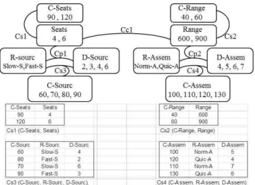
In order to illustrate the problem to solve we recall the very simple example, proposed in [Pitiot et al., 2012], dealing with the configuration and planning of a small plane. The constraint model is shown in figure 2. The plane is defined by two product variables: number of seats (Seats, possible values 4 or 6) and flight range (Range, possible values 600 or 900 kms). A configuration constraint Cc1 forbids a plane with 4 seats and a range of 600 kms. The production process contains two operations: sourcing and assembling. (noted Sourc and Assem). Each operation is described by two pro-cess variables: resource and duration: for sourcing, the re-source (R-Sourc, possible rere-sources “Fast-S” and “Slow-S”) and duration (D-Sourc, possible values 2, 3, 4, 6 weeks), for assembling, the resource (R-Assem, possible resources “Quic-A” and “Norm-A”) and duration (D-Assem, possible values 4, 5, 6, 7 weeks).

Two process constraints linking product and process varia-bles modulate configuration and planning possibilities: one

linking seats with sourcing, Cp1 (Seat, R-Sourc, D-Sourc), and a second one linking range with the assembling, Cp2 (Range, R-Assem, D-Assem). The allowed combinations of each constraint are shown in the 3 tables of figure 2 and lead to 12 solutions for both product and production process.

Figure 2 - Concurrent configuration and planning CSP model

1.2

Optimization needs

With respect to the previous problem, once the customer or the user has provided his non-negotiable requirements, he is frequently interested in knowing what he can get in terms of price and delivery dates (performance is not considered any more). Consequently, the previous model must be updated with some variables and numerical constraints in order to compute the two criteria. The cycle time matches the ending date of the last production operation of the configured prod-uct. Cost is the sum of the product cost and process cost.

Figure 3 - CSP model to optimize

The model of figure 2 is completed in figure 3. For cost, each product variable and each process operation is associ-ated with a cost parameter and a relevant cost constraint: (C-Seats, Cs1), (C-Range, Cs2), (C-Sourc, Cs3) and (C-Assem, cs4) detailed in the tables of figure 3.

The total cost and cycle time are obtained with a numerical constraint as follows:

Total cost = C-Seats + C-Range + C-Sourc + C-Assem. Cycle time = D-Sourc + D-Assem

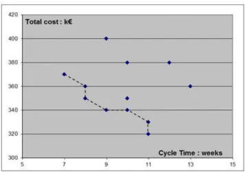
The twelve previous solutions are shown on the figure 4 with the Pareto front gathering the optimal ones. The goal of this article is to improve the computation of this Pareto front with respect to the user preference.

Figure 4 – Problem solutions and Pareto front

2

Optimization problem and techniques

2.1

Optimization problem

The optimization problem can be generalized as the one shown in figure 5.

Figure 5 – Constrained optimization problem

The constrained optimization problem (O-CSP) is defined by the quadruplet <V, D, C, f > where V is the set of deci-sion variables, D the set of domains linked to the variables of V, C the set of constraints on variables of V and f the multi-valued fitness function. The set V gathers: the product variables and the resource process variables (we assume that duration process variables are deduced from product and resource). The set C gathers: only configuration constraints (Cc) and process constraints (Cp). The variables operation durations and cycle time are linked with a numerical con-straint that does not impact solution definition and therefore does not belong to V and C. The same applies to the prod-uct/process cost variables and total cost, which are linked with cost constraints (Cs) and total cost constraints. The filtering system allows dynamically updating the domain of all these variables with respect to the constraints. The varia-bles belonging to V are all symbolic or at least discrete. Du-ration and cost variables are numerical and continuous. Therefore, constraints are discrete (Cc), numerical (cycle time and total cost) or mixed (Cp and Cs). Discrete straints filtering is processed using a conventional arc sistency technique [Bessiere, 2006] while numerical con-straints are processed using bound consistency [Lhomme, 1993].

2.2

Optimization algorithm

A strong specificity of this kind of optimization problem is that the solution space is large. [Amilhastre et al, 2002] re-port that a configuration solution space of more than 1.4*1012 is required for a car-configuration problem. When planning is added, the combinatorial structure can become huge. Another specificity lies in the fact that the shape of the solution space is not continuous and, in most cases, shows many singularities. Furthermore, the multi-criteria problem and the need for Pareto optimal results are also strong problem expectations. These points explain why most of the articles published on this subject, as for example [Hong et al., 2010] or [Li et al., 2006] consider genetic or evolutionary approaches to deal with this problem. In this article we will use “CFB-EA” (for Constraint Filtering Based Evolutionary Algorithm) a promising algorithm that we have designed specifically for this problem.

CFB-EA is based on the SPEA2 method [Zitzler et al., 2001] which is one of the most useful Pareto-based meth-ods. It’s based on the preservation of a selection of best so-lutions in a separate archive. It includes a performing evalu-ation strategy that brings a well-balanced populevalu-ation density on each area of the search space, and it uses an archive trun-cation process that preserves boundary solution. It ensures both a good convergence speed and a fair preservation of solutions diversity.

To deal with constrained problems, we completed this method with specific evolutionary operators (initialization, uniform mutation and uniform crossover) that preserve fea-sibility of generated solutions.

This provides the six steps following approach:

1. Initialization of individual set that respect the con-straints (thanks to filtering),

2. Fitness assignment (balance of Pareto dominance and solution density)

3. Individuals selection and archive update 4. Stopping criterion test

5. Individuals selection for crossover and mutation opera-tors (binary tournaments)

6. Individuals crossover and mutation that respect the con-straints (thanks to filtering)

7. Return to step 2.

For initialization, crossover and mutation operators, each time an individual is created or modified, every gene (deci-sion variable of V) is randomly instantiated into its current domain. To avoid the generation of unfeasible individuals, the domain of every remaining gene is updated by constraint filtering. As filtering is not full proof, inconsistent individu-als can be generated. In this case a limited backtrack process is launched to solve the problem. This approach doesn’t need any additional parameter tuning for constraint han-dling. In the following, we will briefly remind the principles and operators used in CFB-EA.

Many research studies try to integrate constraints in EA. C. Coello Coello proposes a synthetic overview in [Mezura-Montes and Coello Coello 2011]. The current tendencies in the resolution of constrained optimization problem using EAs are penalty functions, stochastic ranking, ε-constrained, multi-objective concepts, feasibility rules and special opera-tors. CFB-EA belongs to this last family.

The special operators class gathers methods that try to deal only with feasible individuals like repairing methods, preservation of feasibility methods or operator that move solutions within a specific region of interest within the search space as for example the boundaries of the feasible region. Generally and has we verified on our last experi-mentations, these methods are known to be performing on non-over-constrained problems (i.e. a feasible solution can be obtained in a reasonable amount of time to be able to generate a population of solutions).

CFB-EA aims at preserving the feasibility of the individuals during their construction or modification. Proposed specific evolutionary operators prune search space using constraint filtering. The main difference between our approach and others is that we do not have any infeasible solution in our population or archive. Each time we modify an individual, the constraints filtering system is used in order to verify consistency preservation of individuals.

Previous experimentations [Pitiot et al., 2012] allowed us to verify that the exact approaches are limited to problems of limited size and that CFB-EA is completely competitive for the level of constraint of the models which interest us. In this article, we propose a new two sub-step optimization approach that takes advantage of the three following charac-teristics: (i) EA are anytime algorithms, e.g. they can supply a set of solutions (Pareto Front) at any time after

initializa-tion, (ii) we have an user who can possibly refine his criteria requirements with regard to the solutions obtained during optimization process ; (iii) CFB-EA is relevant for the range of concurrent configuration and planning problems required (size and constraints level) and more particularly it can pro-pose, in a reasonable amount of time, a good approximation of the Pareto Front that allows the user to decide about his own cost/cycle time compromise.

2.3

Two-task optimization approach.

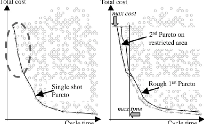
As explained in the introduction, the goal of this article is to evaluate, for large problem, the interest of replacing the single shot Pareto front computation by two successive tasks: (i) a first rough computation that provides a global idea of possible compromises (ii) a second computation on a restricted area selected by the user.

This is shown in the illustration of figure 6. The left part of figure 6 shows a single shot Pareto. The right part of figure 6 shows a rough Pareto quickly obtained (first task), fol-lowed by a zoom selected by the user (max cost and max time) and a second Pareto computation only on this restrict-ed area (second task). The restrictrestrict-ed area is obtainrestrict-ed by con-straining the two criteria total cost and cycle time (or inter-esting area) and filtering these reductions on the whole problem.

Figure 6 – Single shot and two-task optimization principles

The second optimization task does not restart from scratch. It benefits from the individuals of the archive that belongs to the restrained area founded during first task. We thus re-placed the initialization of our CFB-EA (constitution of the first population) by a selection of a set of the best solutions obtained during the first rough optimization.

This provides the following process:

1. Interactive configuration and planning using non-negotiable requirements of the user (as before),

2.1 - 1st global optimization task on negotiable requirements of the user

2.2 - 2nd optimization on interesting area initialized with individuals of the previous step.

Total cost Cycle time Single shot Pareto Total cost Cycle time Rough 1rst _Pareto 2nd _{Pareto on} restricted area max cost max time

3

Experimentations

3.1

Model used and performance measure

The goal of the proposed experiments is to compare these two optimization approaches (single-shot and two-task op-timization approaches) in terms of result quality and compu-tation time. In terms of quality we want to compare the two fronts and will use the Hypervolume measurement proposed by [Zitzler and Thiele 1998] which is illustrated in figure 7. It measures the hypervolume of the space dominated by a set of solutions. It thus allows evaluating both convergence and diversity proprieties (the fittest and most diversified set of solutions is the one that maximizes hypervolume). In terms of computation time, we want to evaluate, for a given Hypervolume result the time reduction provided by the se-cond approach.

Figure 7 – Hyper volume definition

In terms of problem size, we consider a model called “full_ aircraft” that gathers 92 variables (symbolic, integer or float variables) linked by 67 constraints (compatibility tables, equations or inequalities). Among these variables, we find 21 decision variables that will be manipulated by the opti-mization algorithms (chromosome in EAs):

- 12 variables (each with 6 possible discrete values) that describe product customization possibilities,

- 9 variables (each with 9 possible discrete values) that describe production process possibilities. In fact, the nine values aggregate 3 resource types and 3 resource quantities for each of the 9 process operations that compose the production process.

Without any constraints, this provides a number of possible combinations around 1018 (≈ 612 x 99). An average constraint level (around 93% of solutions rejected) allows 7.3*1016 feasible solutions. Results of experimentation’s with other model sizes and other constraint levels can be consulted in [Pitiot et al., 2012].

Figure 8 shows the Pareto Fronts obtained with CFB-EA after 3 and 24 hours of computation. The rough Pareto front obtained after 3 hours of computation allows the user to decide in which area he is interested in. In the next sub-section, we will study a division of this Pareto front in three restricted area:

- Aircraft_zoom_1: area that correspond to solutions with a cycle time less than 410 (solutions with shortest cycle times),

- Aircraft_zoom_2: area that correspond to solutions with a cycle time less than 470 and a total cost less than 535 (compromise solutions),

- Aircraft_zoom_3: area that correspond to solutions with a total cost less than 475 (solutions with lowest total costs).

Figure 8 –Pareto-fronts obtained on “full aircraft model” after 3

and 24 hours of computation

These three areas correspond with a division of the final Pareto front obtained after 24h of computation in three equal parts. These areas have been selected in order to evaluate performance of the proposed two-task approach, but it also corresponds with some classical preference of a user who could wish: (i) a less expensive plane, (ii) a short cycle time, (iii) a compromise between total cost and cycle time. We will discuss this aspect in section 3.3.

The optimization algorithms were implemented in C++ pro-gramming language and interacted with the filtering system coded in Perl language. All tests were done using a laptop computer powered by an Intel core i5 CPU (2.27 Ghz, only one CPU core is used) and using 2.8 Go of ram.

3.2

T

evolutionary settings

For a first experimentation of the two-task approach, we use classical evolutionary settings (e.g. the same evolutionary settings used for the single-shot approach: Population size: 80, Archive size: 100, Individual Mutation Probability: 0.3, Gene Mutation Probability: 0.2, Crossover Probability: 0.8). The main difference with the single-shot approach is with the backtrack limit (e.g. number of allowed backtrack in mutation or crossover operator). This limit has been set to 100 in the one-shot approach and to 30 in the two-step ap-proach.

Indeed in the two-step approach, it could be time consuming to obtain a valid solution. For example with the single-shot optimization, only 2.5% of filtered individuals were unfea-sible and none of them were abandoned; while with the two-task approach and a lower backtrack limit, around 7% of filtered individuals were unfeasible and 0.3% of them were abandoned. So a lower backtrack limit reduces the time spend to try to repair unfeasible individuals.

The only other difference between single-shot CFB-EA and two-task CFB-EA is the stopping criterion. While in single-shot approach, we use a fix time limit (24hours), the two-task approach uses a bcondition stopping test that stops ei-ther if ei-there is no HV improvement after 2 hours or after 12 hours of computation (that must be added to the three initial hours for getting the rough Pareto Front).

3.3

Experimental results

The goal of this section is to evaluate the two-task optimiza-tion on the three selected areas of figure 8 (zoom 1, zoom 2 and zoom3) with respect to the single-shot optimization.

First result illustrations

Figure 9 illustrates an example of the Pareto fronts that can be obtained on the zoom 1 area :

- rough Pareto obtained after 3 hours (fig 9 squares), - two-task, after 3+12 hours (fig 9 triangles),

- single-shot, stopped after 24 hours (fig 9 diamonds).

Figure 9 –Example of Pareto fronts obtained on zoom1

The Pareto Fronts obtained by the two approaches (single-shot and two-task) are very close when the cycle is greater than 355. For lower cycle times, the proposed two-task ap-proach is a little better. However, these curves correspond with a specific run. In order to derive stronger conclusions, 10 executions of the two approaches have been achieved for each of the three zoom areas.

Detailed comparisons

Detailed experimental results achieved on the three zoom areas are presented in figure 10 and table 1.

On each graph of figure, the vertical axis corresponds to the hyper volume (average of ten runs) reach and horizontal one is the time spent. At time 0, the single-shot optimization is launched (dotted line). After 3 hours (10800 seconds): - the single-shot keeps going on (dotted line),

- the two-task is launched (solid line).

The table provides numeric results for each zoom area. The columns display the single-shot, two-task and % gap of: - average final hypervolume,

- average % standard deviation of hypervolume - average computation time,

- average % standard deviation of computation time, - maximum value of hypervolume.

Figure 10 – Evolution of hypervolume

In terms of quality, the new proposed approach (two-task optimization) allows to obtain a similar performance with respect to single-shot one:

- 0.4% worse on zoom1 - 1% worse on zoom2 - 4% better on zoom3

but in around half of computing time: - 13 h instead of 24h for on zoom1 - 13.5h instead of 24h for on zoom2 - 10.5h instead of 24h for on zoom 3.

Furthermore, this computing time includes the 2 hours of computation without any hypervolume reduction before stopping (stopping criterion of the two-task approach).

It can be seen on the figure10 that when the single-shot CFB-EA has trouble to obtain a good Pareto Front during the first three hours, the more the two-task CFB-EA is per-forming. On zoom1 area, single-shot CFB-EA reaches rela-tively quickly a near-final Pareto Front; while on zoom3 area, it reaches it very slowly.

Z o o m 1     Single­shot  CFBEA  Two­task  CFBEA  gap in %  Average  Final HV  5849  5823  ­0.4  Average  HV RSD  3.8%  5.1%    Total  time  86400(24h)  47996 (≈13h)  ­44.6  Total  time  RSD  0  15%    Max HV  6043  6057  0.2  Z o o m 2     Single­shot  CFBEA  Two­task  CFBEA  gap in %  Average  Final HV  1758  1740  ­1.  Average  HV RSD  2.1%  2.3%    Total  time  86400(24h)  48501 (≈13.5h)  ­44  Total  time  RSD  0  16%    Max HV  1795  1776  ­1  Z o o m 3     Single­shot  CFBEA  Two­task  CFBEA  gap in %  Average  Final HV  1765  1844  4.4  Average  HV RSD  3.16%  0.07%    Total  time  86400(24h)  38185 (≈10.5h)  ­55.9  Total  time  RSD  0  26%    Max HV  1831  1845  0,7 

Table 1. Comparison of the two approaches

4 Conclusions

The goal of this paper was to evaluate a new optimization principle that can handle concurrent configuration and plan-ning. First the background of concurrent configuration and planning has been recalled with associated constrained modeling elements. Then an initial optimization approach (single-shot CFB-EA) was described followed by the two-task approach object of this paper.

Instead of computing a Pareto Front on the whole solution space, the key idea is: to compute quickly a rough Pareto

Front, to ask the user about an interesting area and, to launch Pareto computation only on this area.

According to experimental results, in terms of computation time, the new two-task approach allows a significant time saving around half of the previous time needed by the sin-gle-shot optimization approach. In terms of quality, Hyper-volume computation are very close or even a little better in some case.

Furthermore, these results have been obtained on a rather large problem that contains around 1016/1017 solutions. With smaller problems, the proposed approach should perform much better. We are already working on a more extensive test (different model size and different level of constraints) as we did in [Pitiot et al., 2012]. Another key aspect that needs to be study is to find a way to define the rough Pareto computation time.

References

[Aldanondo et al., 2008] M. Aldanondo, E. Vareilles. Con-figuration for mass customization: how to extend prod-uct configuration towards requirements and process con-figuration, Journal of Intelligent Manufacturing, vol. 19 n° 5, p. 521-535A (2008)

[Amilhastre et al, 2002] J. Amilhastre, H. Fargier, P. Mar-quis, Consistency restoration and explanations in dynam-ic csps - appldynam-ication to configuration, in: Artifdynam-icial Intel-ligence vol.135, 2002, pp. 199-234.

[Bartak et al., 2010] R. Barták, M. Salido, F. Rossi. Con-straint satisfaction techniques in planning and schedul-ing, in: Journal of Intelligent Manufacturschedul-ing, vol. 21, n°1, p. 5-15 (2010)

[Bessiere, 2006] C. Bessiere, Handbook of Constraint Pro-gramming, Eds. Elsevier, chap. 3 Constraint propaga-tion, 2006, pp. 29-70.

[Hong et al., 2010] G. Hong, D. Xue, Y. Tu,, Rapid identifi-cation of the optimal product configuration and its pa-rameters based on customer-centric product modeling for one-of-a-kind production, in: Computers in Industry Vol.61 n°3, 2010, pp. 270–279.

[Junker, 2006] U. Junker. Handbook of Constraint Pro-gramming, Elsevier, chap. 24 Configuration, p. 835-875 (2006)

[Laborie, 2003] P. Laborie. Algorithms for propagating re-source constraints in AI planning and scheduling: Exist-ing approaches and new results, in: Artificial Intelli-gence vol 143, 2003, pp 151-188.

[Lhomme, 1993] O. Lhomme. Consistency techniques for numerical CSPs, in: proc. of IJCAI 1993, pp. 232-238. [Li et al., 2006] L. Li, L. Chen, Z. Huang, Y. Zhong,

Prod-uct configuration optimization using a multiobjective GA, in: I.J. of Adv. Manufacturing Technology vol. 30, 2006, pp. 20-29.

[Montes and Coello Coello 2011] E. Mezura-Montes, C. Coello Coello, Constraint-Handling in Na-ture-Inspired Numerical Optimization: Past, Present and Future, in: Swarm and Evolutionary Computation, Vol. 1 n°4, 2011, pp. 173-194

[Mittal and Frayman, 1989] S. Mittal, F. Frayman. Towards a generic model of configuration tasks, proc of IJCAI, p. 1395-1401(1989).

[Pitiot et al., 2012] P. Pitiot, M. Aldanondo, E. Vareilles, L. Zhang, T. Coudert. Some Experimental Results Relevant to the Optimization of Configuration and Planning Prob-lems, in : Lecture Notes in Computer Science Volume 7661, 2012, pp 301-310

[Pitiot et al., 2013] P. Pitiot, M. Aldanondo, E. Vareilles, P. Gaborit, M. Djefel, S. Carbonnel, Concurrent product configuration and process planning, towards an approach combining interactivity and optimality, in: I.J. of Pro-duction Research Vol. 51 n°2, 2013 , pp. 524-541. [Schierholt 2001] K. Schierholt. Process configuration:

combining the principles of product configuration and process planning AI EDAM / Volume 15 / Issue 05 / no-vembre 2001 , pp 411-424

[Soininen et al., 1998] T. Soininen, J. Tiihonen, T. Männis-tö, and R. Sulonen, Towards a General Ontology of Con-figuration., in: Artificial Intelligence for Engineering Design, Analysis and Manufacturing vol 12 n°4, 1998, pp. 357–372.

[Zhang et al., 2013] L. Zhang, E. Vareilles, M. Aldanondo. Generic bill of functions, materials, and operations for SAP2 configuration, in: I.J. of Production Research Vol. 51 n°2, 2013 , pp. 465-478.

[Zitzler and Thiele 1998] E. Zitzler, L. Thiele, Multiobjec-tive optimization using evolutionary algorithms - a com-parative case study, in: proc. of 5th Int. Conf. on parallel problem solving from nature, Eds. Springer Verlag, 1998, pp. 292-301.

[Zitzler et al., 2001] E. Zitzler, M. Laumanns, L. Thiele., SPEA2: Improving the Strength Pareto Evolutionary Al-gorithm, Technical Report 103, Swiss Fed. Inst. of Technology (ETH), Zurich (2001)