Journal of Fundamental and Applied Sciences is licensed under aCreative Commons Attribution-NonCommercial 4.0 International License.Libraries Resource Directory. We are listed underResearch Associationscategory.
THE SUBSTANTIAL MODEL OF THE PHOTON
Sergey G. Fedosin
Sviazeva Str. 22-79, Perm, 614088, Perm Krai, Russian Federation
Received: 05 September 2016 / Accepted: 27 December 2016 / Published online: 01 January 2017 ABSTRACT
It is shown that the angular frequency of the photon is nothing else than the averaged angular frequency of revolution of the electron cloud’s center during emission and quantum transition between two energy levels in an atom. On assumption that the photon consists of charged particles of the vacuum field (of praons), the substantial model of a photon is constructed. Praons move inside the photon in the same way as they must move in the electromagnetic field of the emitting electron, while internal periodic wave structure is formed inside the photon. The properties of praons, including their mass, charge and speed, are derived in the framework of the theory of infinite nesting of matter. At the same time, praons are part of nucleons and leptons just as nucleons are the basis of neutron stars and the matter of ordinary stars and planets. With the help of the Lorentz transformations, which correlate the laboratory reference frame and the reference frame, co-moving with the praons inside the photon, transformation of the electromagnetic field components is performed. This allows us to calculate the longitudinal magnetic field and magnetic dipole moment of the photon, and to understand the relation between the transverse components of the electric and magnetic fields, connected by a coefficient in the form of the speed of light. The total rest mass of the particles making up the photon is found, it turns out to be inversely proportional to the nuclear charge number of the hydrogen-like atom, which emits the photon.
Keywords: matter waves; quantum gravity; electromagnetic interaction; magnetic moments;
properties of photon.
Author Correspondence, e-mail:[email protected]
doi:http://dx.doi.org/10.4314/jfas.v9i1.25 ISSN 1112-9867
1. INTRODUCTION
As is known, the more elementary the particle is, the less we know about it. The photon, the concept of which appeared more than a hundred years ago in the writings of Albert Einstein, is not an exception. What seems surprising about this particle is the absence of the rest mass, but at the same time the presence of wave and corpuscle properties, high stability and the ability to travel over cosmic distances with low energy losses, the indissoluble connection between photons and charged particles in the processes of absorption and emission.
One of the modern methods of studying the photon structure is experiments on colliding photons with each other, with protons and electrons. These experiments show that at small distances a photon can be modelled in the form of fluxes of quarks and gluons [1]. These fluxes should participate in interactions as is prescribed in quantum electrodynamics.
In the oscillating model [2] a photon is regarded as an object periodically changing its volume, the speed of which is less than the speed of light. In this model, it is assumed that the rest mass of the photon with the greatest wavelength can be related to the initial conditions of the early Universe. Based on this assumption the estimate of the mass of the photon’s inner part is made:
67
0 1.6 10
m kg. In contrast, in [3] it is considered that a photon has no proper mass, however under the influence of the vacuum field the effective mass appears.
In [4] the photon diameter is deemed equal to the wavelength on the ground that this dimension is the limit for the wave diffraction. The soliton model of the photon is constructed in [5], where the equation for the vector potential is used, which is similar to the generalized Schrödinger equation. In [6] it is indicated that the drawback of the soliton model is the difficulty to explain the origin of the soliton, which usually requires a nonlinear medium. The photon diameter according to [7] is equal to , and outside of the photon its field strength/ must decrease in inverse proportion to the distance to the photon’s axis. This allows the photon to undergo interference in the Young's interference experiment. Description of a photon as a rotating particle in the framework of quantum electrodynamics is presented in [8].
Due to the lack of key information about the internal parameters of electromagnetic quanta, the existing models still require further development and specification, because they do not allow us to define concretely the actual structure of a photon, to relate it to the source of emission at
the atomic level and to the experimental data. The purpose of this article is to fill this gap and to provide a more detailed and well-grounded substantial model of the photon. We will do it based on the theory of infinite nesting of matter and the substantial model of the electron [9].
We will start with considering the basic conditions of emission from a hydrogen-like atom and estimating the duration of emission, which is necessary to determine the photon’s length in space and then to calculate its energy density. In Section 3, we will present the main components of the electric and magnetic fields that are created by the charge rotating around the nucleus in the near and wave zones. The energy flux of these fields leads to a standard formula for the charge emission. Our goal is to use certain electromagnetic field components of the rotating charge to find the equations of motion for the smallest charged particles of the vacuum field in Section 4. We consider these particles, called praons, as construction material not only for photons but also for any other elementary particles, including nucleons and leptons. Praons have mass and we use the Lorentz factor to describe their motion at relativistic velocities. This allows us to turn with the help of Lorentz transformations to the reference frame, co-moving with praons, and to understand their motion from the standpoint of a fixed photon.
In Section 5, based on the motion of praons in the electromagnetic field of the emitting electron, periodically changing in space and time, we construct the substantial model of the photon. Section 6 concerns the structure of the electromagnetic field and the strong gravitational field inside the photon and their interaction with praons, which ensures the photon’s stability. In Sections 7, 8, 9 we derive the Lorentz factor for praons and the energy fluxes within the photon, the magnetic dipole moment, and the rest mass of the particles that make up the photon, respectively.
2. EMISSION OF A PHOTON FROM A HYDROGEN-LIKE ATOM
According to the Bohr relation, the energy of a photon as an electromagnetic quantum, emitted during the electron’s transition from some energy level i to a lower level j , equals the difference between the total energies of the electron at these levels:
i j i j
here is the Dirac constant,
i j
is the angular frequency of the photon.
But how could we describe more clearly what is happening in the atom during emission of the quantum? For simplicity, let us assume that one electron is located in the central-type field of the hydrogen-like atom. If the electron matter rotates totally symmetrically relative to the nucleus, then the electron would not emit. This is due to the fact that for each charge element of the electron matter in an axisymmetric configuration there is a similar charge element on the opposite side of the axis, which is moving in the opposite direction. At large distances, the contribution of the nucleus and of these charge elements into the total electric field strength E
and the magnetic induction B will be compensated, and the resulting energy flux will be close
to zero.
Therefore, in order to produce emission the electron must move so that its center of inertia is sufficiently removed from the nucleus. Let us assume that the center of the electron cloud rotates at a distance r from the nucleus and is held in relative equilibrium by a force directed
towards the nucleus. If the velocity of the cloud’s center is equal to u , then for the equality of the central and centripetal forces we can write:
2 2 0 4 c Z e F r , 2 2 2 0 4 e m u Z e r r , (2)
where Z is the number of protons in the nucleus, e is the elementary charge, is the0 vacuum permittivity, m is the electron mass, so thate F is the electric force between thec
positively charged nucleus with the charge Z e and the negatively charged electron.
In (2) we used the approximately equal symbol, since in case of emission the distance r will
in the intrinsic electromagnetic energy of the cloud due to the change in the radius and volume of the cloud as it approaches the nucleus. Then we use the standard formula for the power of the total electromagnetic emission from the elementary charge, rotating around a certain center [10]. If we consider the emitted energy per time dt up to the sign equal to the change in the total energy dE of the electron cloud, then we can write:e
2 4 2 3 0 6 e dE e r dt c , (3)
here c is the speed of light, and a small coefficient reflects the fact that the emission from the electron cloud as a dimensional figure should differ from the emission from of the rotating electron as a point.
Assuming that ur, where is the angular velocity of rotation of the electron cloud’s
center around the nucleus, from the ratio for the power e e dE
F u
dt and (3) we will find the
magnitude of the force, decelerating the cloud’s rotation:
2 3 3 2 0 6 e e u F c r . (4)
For the angular momentum of the cloud’s center of mass and its rate of change under the influence of the force moment Fer we can write:
e
Lm ur, e
dL
F r
dt . (5)
e e e dE dL F u F r dt dt , e dE dL , (6)
i.e. the change in the electron cloud’s energy with the change in the angular momentum of the cloud’s center is proportional to the angular frequency of rotation.
Expressing from (2) the rotation speed in the form
2 0 4 e Z e u m r and substituting in (5), in
view of (4) we arrive at the differential equation for the dependence of the distance r on the
time: 2 3 2 5 5 2 5 2 3 3 2 5 2 0 0 4 48 e e Z e m r d Z e dt c m r , 1 3 4 3 0 2 2 3 2 0 4 e Z e t r r c m ,
2 2 3 2 5 5 6 3 3 3 6 6 0 0 4 4 10 4 256 . e i j e c m c r r i j Z e Z e m (7)here r is the distance to the cloud’s center at the initial time.0
Expression (7) approximately describes the small changes in the distance r over time for the
rotational motion of the electron cloud. Besides the following condition must hold: r0,
2 2 3 2 3 0 0 0 4 4 c m re t t Z e
, where t is the time of the cloud’s center of mass falling onto the0
attracting center.
For example, if we assume that the distance changes from r0 ri 4aB to r rj aB, where
B
1
j at 1 and Z 1 from (7) we obtain the value of the order of 9.8 10 10s, that is the typical time of the electromagnetic quantum emission by the electron in atomic transitions. If we substitute the distance (7) in (3), taking into account
2 0 4 e Z e u r m r , and integrate
it over the time, we will find the total energy of the electron cloud:
2 0 8 e Z e E const r . (8)
From (8) we see that if the electron moves from the energy level i at the energy level j , then the energy of the emitted electromagnetic quantum will amount to the value equal to the difference between the electron’s energy levels in the atom:
2 2 0 0 8 8 i j i j Z e Z e E E r r . This
relation fully coincides with the Bohr condition for energies. This should have been expected, because from (2) it follows that the electrostatic energy of the electron at the level i is equal to the value 2 0 4 i i Z e W r
, and the kinetic energy of the electron is
2 2 0 2 8 e i i i m u Z e K r . The
total energy at the level i is supposed to be equal to the sum of these energies:
2 0 8 i i i i Z e E W K r .
From the condition
2 0 4 e Z e u r m r
and (3) it follows that the power of the energy
emission is strongly dependent on the current distance r :
2 6 3 3 3 2 4 0 96 e e dE Z e dt c m r . (9)
According to (9) we can assume that the basic energy of the electromagnetic quantum during the transition from the energy level i to the energy level j is emitted by the electron cloud near the level j , where the radius of rotation r of the electron cloud’s center is less. In this
case, we find explanation for the fact that the frequency of electromagnetic quanta i j in (1) is
close, but always less than the frequency of the electron cloud’s rotation near the energy level
j . If we consider at some time point the emitted electromagnetic quantum along its length in
space, then its oscillation frequency should increase when moving from the front part of the quantum to its rear part, and the quantum energy density must reach the maximum closer to the rear part of the quantum.
The constant h2 was introduced by Planck in 1900 while establishing the law of energy distribution in the blackbody spectrum. This constant turned out to be a universal quantity at the level of elementary particles and atoms, with the dimensionality of a quantum of action. Its role in determining the electromagnetic energy of quanta, despite the fact that the wave oscillation frequency inside these quanta in our opinion cannot be strictly constant, is quite similar to that of the Boltzmann constant in determining the average thermal energy of a set of particles through the temperature, with the energy spread of individual particles, which is always present.
We will show that the angular frequency i j of the quantum is the averaged angular frequency of rotation of the electron cloud’s center at transition between the energy levels i and j . For in view of (6) we have:
1 1 . j j i i L L j i e e j i L j i L j i E E E dL dE L L L L L L L
At L the energy electromagnetic quantum is:
e
From comparison of (10) and (1) we see that i j . However, if for some reason L ,
the equality i j would not exist.
Since during the emission of quanta the electron’s angular momentum changes, the change in the angular momentum should be carried away by the electromagnetic quantum. Photons or electromagnetic quanta, are attributed the angular momentum, equal to . Therefore, during emission the electron loses the angular momentum of the order of and the same angular momentum is acquired by the photon; the electron loses the energy of the order of h , where
is the average rotation frequency of the electron’s center of mass near the nucleus for the
period of emission, and the photon acquires this energy. The electron acts in this case as a carrier particle that transfers its kinetic energy and angular momentum into the energy and angular momentum of the electromagnetic wave that are concentrated in the emitted photon.
3. THE EMISSION FROM THE ROTATING POINT CHARGE
Let us assume that a charged point particle with the charge q rotates by a circle of radius R0
with the angular velocity and the orbital velocity V0 R0. We will place a spherical reference frame at the center of this circle and will seek for the components of the electromagnetic field strength from the rotating charge at some remote point with the radius-vector R( , , )x y z . The current position of the charge is given by the vector
0 (R0cost R, 0sint, 0)
R , so that the circle of rotation lies in the plane XOY .
In order to determine the electric field strength E and the magnetic field induction B in the
first approximation we will use the formulas that take into account any motion of the charge in the special theory of relativity:
2 2 2 2 2 0 1 4 r r r q r d d r c dt r c dt e e E e , 1 r c B e E , (11)
here r R R0( )t is the vector from the charge to the remote point at the early time point c r t t ,
2 2 0 2 0cos t y Rsin t z R x r , 0cos 0sin , , r x R t y R t z r r r e is the unit vector, directed from the charge to the
remote point, taken for the case of rotation of this charge by a circle at an early time point t.
The formula (11) was first published by Oliver Heaviside in 1902. It was independently discovered by R. P. Feynman, in about 1950, and given in some lectures as a good way of thinking about synchrotron radiation [11].
From the definitions of t and r we see that they are mutually dependent. We will take for them the derivatives with respect to time:
1 1 dt dr dt c dt , dr R0
xsin t ycos t
dt dt r dt ,and then we will express these derivatives independently from each other:
0 1 1 sin cos dt R dt x t y t c r ,
0 0 sin cos 1 sin cos R x t y t dr r R dt x t y t c r .If the orbital velocity V0 R0 is significantly less than the speed of light c, as is the case for the electron in the atom, we see that:
1 dt dt , 0 dr R dt . (12)
Taking the first time derivative of the unit vector of the original direction, we find: dt r d r t R x dt t d r t R dt derx 2 0 0sin cos , dt r d r t R y dt t d r t R dt dery 2 0 0cos sin , dt r d r z dt derz 2 . (13)
Let us substitute in the right-hand side of (13) the time derivatives by their maximum values according to (12) and calculate the second time derivatives of the unit vector:
2 2 2 2
0 0 0 0 0
2 2 2 3
cos sin sin 2 ( cos )
. r x d e R t dt R t dr R t dt R x R t dr dt r dt r dt r dt r dt 2 2 2 2 0 0 0 0 0 2 2 2 3
sin cos cos 2 ( sin )
. r y d e R t dt R t dr R t dt R y R t dr dt r dt r dt r dt r dt 2 0 2 3 2 r z d e R z dr dt r dt . (14)
For the components of the derivative d r2 dt r e
in (11), in view of (12) and (13), we obtain:
0 0 2 2 3 3 4 2 sin 2( cos ) 1 . r x r x r x e de e R t x R t d dr dr dt r r dt r dt r r dt 0 0 2 2 3 3 4 2 cos 2( sin ) 1 . r y r y r y e de e R t y R t d dr dr dt r r dt r dt r r dt
2 3 4 3 r z e d d z z dr dt r dt r r dt . (15)
Substituting (14) and (15) in (11), we find the component of the electric field strength E :x
2 0 0 0 0 3 2 3 2 2 2 0 0 0 0 0 2 2 2 2 3 2
cos sin 2( cos ) cos
.
4 sin sin 2 ( cos )
x x R t R t x R t dr R t q r r c r c dt r c E R t dr R t dt R x R t dr r c dt r c dt r c dt (16) According to (12), 0 0 dr R V dt
, and then in (16) the third and seventh terms are less than
the first term, since V0 c. Similarly, taking into account the relation dt 1
dt
, the fifth and sixth terms in (16) are always less than the second term. As a result, leaving the greatest terms in (16) and (11), for the electromagnetic field components we have the following:
2
0 0 0
3 2 2
0
cos sin cos
4 x x R t R t R t q E r r c r c . 2 0 0 0 3 2 2 0
sin cos sin
4 y y R t R t R t q E r r c r c . 0 3 3 3 2 3 0 0 2 3 . 4 4 z R z q z z dr dr q z E r r c dt r c dt r (17) 2 0 0 3 2 2 3 0 cos sin 4 x R z t R z t q B r c r c , 2 0 0 3 2 2 3 0 sin cos 4 y R z t R z t q B r c r c ,
2
0 0
0
3 2 2 3
0
cos sin sin cos
4 z R R q B R x t y t x t y t r c r c .
At large distances, when r c , the last terms containing r in the denominator start predominating in the electric field components (17), and the terms containing r2 in the denominator start predominating in the magnetic field components.
The Poynting vector or the electromagnetic energy flux equals:
2
0 [ ] p c
S E B .
If in (17) we take into account only the last terms that remain at a great distance, then the Poynting vector components are as follows:
2 2 2 2
0 0
2 3 2 2
0
sin ( sin cos ) cos
16 p x q R R t x t y t z t S r c c r , 2 2 2 2 0 0 2 3 2 2 0
cos ( sin cos ) sin
16 p y q R R t x t y t z t S r c c r , 2 4 2 0 2 3 3 0 16 p z q R z S r c .
We must first average the components Sp x and Sp y for one period of the charge’s rotation, when the phase t varies from 0 to 2 . Given that Sp z Sp z, we have:
2 2 4 2 0 2 3 3 0 0 1 2 32 p x p x q R x S S d r c
, 2 2 4 2 0 2 3 3 0 0 1 2 32 p y p y q R y S S d r c
.Now, integrating Sp over the surface of the remote sphere we find the rate of the electromagnetic energy flux, averaged over the period:
2 4 2 2 2 2 2 4 2 0 0 2 3 3 3 0 0 2 . 32 6 em p dW q R x y z q R d d dt c Rr c
S n
(18) here x, y z, R R R n is a unit vector perpendicular to the sphere surface, d R2sin d d
is an area unit, for the spherical coordinates x2y2z2 R2, zRcos and we assumed that r R.
The emission rate in (18) coincides with the result in (3), while for calculation instead of full expressions for the field we used only the field components from (17) that remain in the remote area.
4. PHOTON FORMATION
4.1. The near zone
We consider an electron in an atom as a flat disk, the center of which is shifted relative to the nucleus and is rotating around the nucleus during emission of a photon. After formation, a photon becomes an independent object and no longer depends on the fields generated by the emitting electron and the atomic nucleus. Now we need to build a model of a photon, to understand what it consists of, how it maintains the perpendicular structure of the electromagnetic field and why a photon is a stable object. For this purpose, we will turn to the results of [12,13], where the photon is regarded as an object consisting of tightly bound charged particles.
In [14] we assume the positively and negatively charged praons as the charged particles that permeate entire space in different directions and create the interaction forces between the electric charges. These particles are one of the components of the vacuum field, along with the graviton field, responsible for the occurrence of gravitational forces [15] in Le Sage’s model. The mass to charge ratio found for praons turns out to be such as it follows from the coefficients of similarity between different levels of matter and from the theory of dimensions. According to
the theory of infinite nesting of matter, praons make up the matter of nucleons just as nucleons make up the matter of neutron stars. Besides, the fluxes of charged praons are the cause of the Coulomb force, and inside of photons praons come into a state of steady and orderly rotation. In the substantial model of electron [9], in a hydrogen atom in its ground state the average radius of the electron disk is assumed to be equal to the Bohr radius a , the minimum radius ofB
the disk is 0.5aB and the maximum radius reaches 1.5a . These radii correlate with theB
electron density distribution according to the electron wave function and the solutions of Schrödinger equation. Close to the nucleus, at a radius less than 0.5a , the electron matterB
density decreases rapidly. We suppose that the fluxes of praons pass here along the axis OZ, perpendicular to the plane of the electron disk, without direct contact with the electron matter, interacting with the nucleus and electron only by means of the field. From the symmetry of fields of the nucleus and electron disk it follows that near the axis OZ the praon fluxes mostly move linearly, creating the basis of the emitted photon. Other praons that pass through the electron disk, after interaction with the charged matter of the disk, get into the photon shell with a cross-section of the order of the electron disk’s size. The same pattern holds for the hydrogen-like atom.
For example, in [14] at a first approximation a photon is considered as a long, thin cylinder, rotating at the angular frequency 2 c
, where is the wavelength of the photon. For a
photon with the wavelength 1.21567 10 7m and the angular frequency 1.54946 10 16 s-1, which emerges in the hydrogen atom at the transition of the electron from the second to the first level in the Lyman series, we assume the average radius of the electron disk 4aB as the photon radius. The total length of the photon is given by the expression c, where is the duration of the photon emission by the atom, according to (7).
Let us analyze the electromagnetic field components at an arbitrary point in space ( , , )x y z
R , the coordinates x and y of which do not exceed much the orbit radius R of0
orbit radius: z . In this area, the condition r cR0 holds, so that in (17) the first terms predominate. Turning to the hydrogen-like atom, in (17) we will also replace q with the negative charge of the electron e, where e is the elementary charge, and will add to (17) the static electric field components from the charge Z e of the atomic nucleus, located in the center of the coordinate system. The result for the field components can be written as follows:
0 3 0 ( 1) cos 4 x Z ex eR t E r , 30 0 ( 1) sin 4 y Z e y eR t E r , 3 0 ( 1) 4 z Z ez E r . (19) 0 3 2 0 cos 4 x e R z t B r c , 0 3 2 0 sin 4 y e R z t B r c ,
0 0 3 2 0 cos sin 4 z e R R x t y t B r c .The magnetic field component B in (19) oscillates in a complicated way. If we restrictz
ourselves to an area, where z R0, that is outside the atom, but with the near zone condition
r c
, then we can assume Rr and r z . In this case, the component B can bez
neglected, since it would be z R times less than the components/ 0 B andx By.
The electric field components, depending on the multiplier Z1, determine the constant field from the effective charge (Z1)e of the hydrogen-like atom, decreasing with the distance according to the Coulomb's law. This field should accelerate the charged praons, changing their energy. However, the emerging photon has the almost same number of positive and negative praons, which ensures the electroneutrality of the photon. These praons also interact strongly with each other and are in a bound state. Then the component E at sufficiently large distancesz
As a result, the pattern of the moving field will be formed mainly by those components in E ,x
y
E , B andx By that are time-dependent. Introducing the transverse vectors E (E Ex, y, 0) and B (B Bx, y, 0), from (19) we find for those components the following:
0 0 3 0 ˆ ( ) 4 eR t r E R , 0 0 3 2 0 ˆ ( ) 4 e R z t r c B R , (20)
where the unit vector Rˆ (0 t)(cost,sint, 0) determines the position of the rotating electron in the plane XOY at the early time point t.
From (20) we see that the transverse components of the electric E and magnetic B fields rotate around the axis OZ at the angular frequency synchronously with the rotation of the vector Rˆ (0 t) and with the rotation of the electron in the atom. At the same time the component E is directed in space the same way as the radius vector of the electron at the
early time, and the magnetic field B is directed oppositely.
We will write down the equation of motion of the negatively charged praons in the external electromagnetic field and will find the mode of their motion, using the general equations of motion in the same way as in [16,17]. The equation of motion with respect to the early time t is determined by the Lorentz force:
( ) pre pr pr d m e e d t V E V B , (21)here mpre is the invariant mass of a negatively charged praon,
2 2
1
1 V c
pr
e is the elementary charge for praon level of matter,
V is the particle velocity vector.
After substitution of the fields (20) into (21), we obtain for the motion of particles the following: 0 0 3 3 2 0 0 ( ) cos ( ) sin ( ) 4 4 pr pr z x pre pre ee R ee R zV d V t t d t m r m r c , 0 0 3 3 2 0 0 ( ) sin ( ) cos ( ) 4 4 pr pr z y pre pre ee R ee R zV d V t t d t m r m r c , 0 3 2 0 ( ) sin ( ) cos ( ) 4 pr z x y pre ee R z d V V t V t d t m r c . (22)
We will take into account that the Lorentz force components in (22), containing c in the2
denominator, can be excluded from calculation because they are much less than the components without the speed of light. From the ratio of these components the condition follows:
2 z
z V c
. The velocity of praons V along the axis OZ reaches almost the speed of light,z
so that the condition has the form z c, which corresponds to the previously accepted expression r c for the near zone. Consequently, an approximate solution to the equations (22) for the particles’ velocity has the form:
0 3 0 sin ( ) 4 pr x pre ee R V t m r , 0 3 0 cos ( ) 4 pr y pre ee R V t m r , Vz const.
What would change, if at these velocities we will take into account that the electric field components (19) also contain constant terms, containing the multiplier Z1? If the action of
the field component E can be neglected, then taking into account the constant terms in thez
components E andx Ey leads to emerging of an additional centripetal force. This force influences the negative praons and changes their velocity on the stable rotation trajectory up to the following values:
0 3 2 0 sin ( ) 4 ( 1) pr x pre pr ee R t V m r ee Z , 0 3 2 0 cos ( ) 4 ( 1) pr y pre pr ee R t V m r ee Z , Vz const. (23)
For the hydrogen atom Z 1 and the expressions for velocities are simplified. In this case, from (23) we see that in the near zone at the time t, which does not exceed the period of the electron’s rotation around the nucleus, the negative praons rotate around the axis OZ at velocity Vpre following the electron’s rotation in the atom. For the positive praons, at the same
angular velocity vector, the linear velocity components in (23) will be in opposite direction relative to the velocity components of the negative praons, due to a different sign of charge. For such motion, it is enough for the negative praons to rotate on the same side as the electron at the early time and for the positive praons to be on the opposite side relative to the axis OZ , at equal common rotation. We can also take into account that the negative praons at their matter level are the analogues of electrons and therefore the mass ratio of positive and negative praons is
equal to the mass ratio of proton and electron: pr p
pre e
m m
m m . Substituting mpr instead of mpre
in (23) leads to the fact that the velocities and radii of rotation of the positive praons will be significantly less than those of the negative praons.
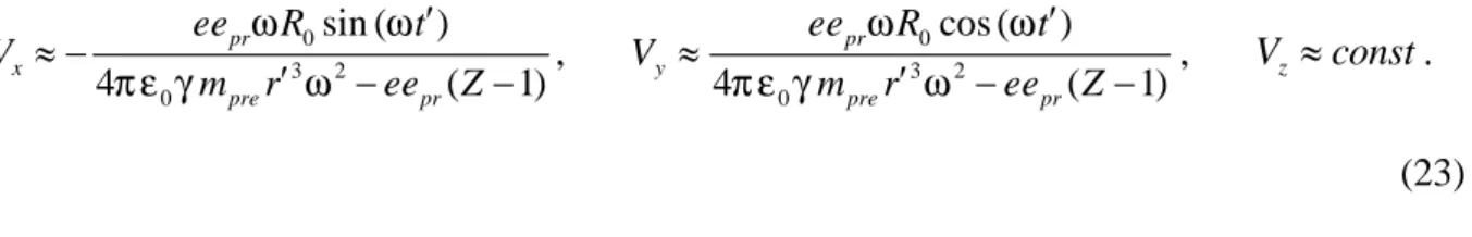
Figure 1 shows a surface perpendicular to the axis OZ and shifted along this axis for a certain distance from the atom, on which we can see the directions of the electric and magnetic fields (20) and the velocities of praons according to (23) for the hydrogen atom at Z 1. All vectors correspond to the time point t, at which the condition t 2n is met, where n1, 2,3... The vector Vpr stands for the velocity of the positive praons.
4.2. The wave zone
Let us now consider another extreme case, when the coordinate z is in the remote wave zone.
Here the properties of the emerging photon should reveal themselves to the full extent. If we consider the electric field strength components in (17), we see that among all the terms those terms become the maximum terms, which contain the square of the speed of light. These terms slowly decrease with the distance, because they contain the distance r to the first power in the denominator. In the magnetic components, the largest terms also slowly decrease with the distance, since they are proportional to the multiplier z2
r .
Turning again to the hydrogen atom, we will replace q in (17) with the electron’s negative charge e and will add to (17) the components of the static electric field from the charge
Z e
of the atomic nucleus, located in the center of the coordinate system. As a result, the field components in the wave zone can be expressed as follows:
Fig. 1. The fields (20) and velocities (23) of praons close to the axis OZ in the near zone at t 2n for the hydrogen atom.
z x y E B Vpre Vpr
2 0 3 2 0 0 cos ( 1) 4 4 x e R t Z ex E r r c , 2 0 3 2 0 0 sin ( 1) 4 4 y e R t Z e y E r r c , 3 0 ( 1) 4 z Z ez E r . (24) 2 0 2 3 0 sin 4 x e R z t B r c , 2 0 2 3 0 cos 4 y e R z t B r c ,
2 0 2 3 0 sin cos 0 4 z e R B x t y t r c .We will consider sufficiently long distances r, when the conditions
0 (Z 1) x r c R , 0 (Z 1) y r c R
are met. Then in the components E andx Ey in (24) we can neglect the
constant terms from the nuclear field. As for component E , it should have little effect on thez
photon’s motion also due to its electrical neutrality.
The magnetic field component B as compared with the componentsz B andx By is small.
For example, the amplitude ratio of the components Bz and Bx at small x and y is
estimated as z 0 1
x
x R
B
B z z . Further on we will consider that the component B is close toz
zero and in the wave zone it is not involved in the processes inside the photon. Then the electric and magnetic fields that remain in (24) would be perpendicular to each other and to the axis
OZ , besides the magnetic field components would be shifted forward relative to the electric
field components at an angle 2 and rotate at the same frequency . In addition, the relation
x y
E cB appears. In a photon the same conditions are met, and it is expected that the fields in the form of (24) should form a circularly polarized photon, that is, with rotation of the electric vector relative to the photon’s axis.
In (24) we will turn from the earlier time t to the current time t in the laboratory reference frame, taking into account the definition: t t r
c
with the amplitude k 2 c
, which is directed along the axis OZ , so that at any sign of the coordinate z and velocity of praons Vz the following relations are satisfied: k z0,
0 z kV . Then t t r t z t k z c c
, and for periodically varying fields we can
write the following:
cost cos (tk z), sint sin (tk z), RˆE [cos(t k z ),sin (t k z ),0],
ˆ [ sin ( ),cos( ),0] B tk z tk z R , 2 0 2 0 ˆ 4 E e R r c E R , 2 0 2 3 0 ˆ 4 B e z R r c B R . (25)
As we can see, at any constant value r z , the fields in (25) depend on the time according to the sine law. In addition, as the coordinate z increases at the points, where the condition zn is satisfied and n1, 2,3..., the fields (25) rotate synchronously with each other along the axis OZ. Thus, the field acquires a periodic spatial structure, repeated after a minimum distance equal to the wavelength. In the previous case, when equation (21) was solved, the spatial structure was not considered, as we were considering the near zone, the size of which is of the order of less than one wavelength.
Similarly to (21), we will write the equation of motion for the negative praons, but with respect to the current time t :
( ) pre pr pr d m e e d t V E V B .2 0 2 0 ( ) ( ) ( ) cos ( ) 1 4 pr z x x x pre ee R zV d V V V t k z d t t m r c r c V , (26) 2 0 2 0 ( ) ( ) ( ) sin ( ) 1 4 pr z y y y pre ee R zV d V V V t k z d t t m r c r c V , 2 0 2 3 0 ( ) ( ) ( ) cos ( ) sin ( ) 4 pr z z z x y pre ee z R d V V V V t k z V t k z d t t m r c V .
In the right side of (26) the Lorentz force depends on two variables – the time t and the coordinate z that define the distance to the emitting atom. Therefore, during the motion of the
charged particles in the electromagnetic field, the acceleration and velocity of the particles also become the functions of t and z . Due to this, we presented the time derivatives in the left side
of (26) as material derivatives.
The change of z has a more significant impact on the argument of sines and cosines than the
change of r in the amplitude’s denominator. If we consider z as a variable only in the sines
and cosines, then the approximate solution of equations (26) for the velocity of the particles has the form: 0 2 0 sin ( ) 4 pr x pre ee R V t k z m r c , 0 2 0 cos ( ) 4 pr y pre ee R V t k z m r c , Vz const. (27)
If the time t is fixed, then in case of changing the position of the coordinate from zn to
( 1)
z n , the velocity vector in (27) will make complete revolution around the axis OZ, while at large n the decrease of the velocity amplitude due to the change of r will be little. This proves our approximate solution of (27), though solving the equations we have not taken into account the change of z in r in the denominator of the Lorentz force’s amplitude.
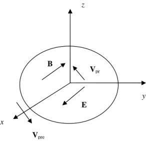
Figure 2 shows a surface perpendicular to the axis OZ , where the directions of the electric and
magnetic fields (25) and praons’ velocities are shown according to (27). The vectors Vpr and
pre
V denote the velocities of the positive and negative praons, respectively.
Let us pay attention to the difference between the solutions (23) and (27), which consists in the
fact that the praons’ velocities in them for the hydrogen atom at Z 1 have different signs. In
this case, at the boundary between the near and wave zones, which is reflected by the condition
r c
, a change of the field action takes place. Specifically, the total field of the electron changes its phase to the opposite, due to the increased field components (25) in comparison with the field components (20). As a result, when the electron is rotating on the one side from the axis OZ, the negative praons are located and rotating under the field action on the opposite side of the axis OZ. As for the positive praons, they are now located on the side, where the electron is moving, and are rotating at lower speed and with a smaller radius of rotation, due to their large mass.
Additionally, the photon obtains spatial structure in the wave zone. How can it be explained from the standpoint of physics? Assume that the electromagnetic field of the electron, which is
Fig. 2. The fields (25) and velocities (27) of the praons near the axis OZ in the remote wave zone at t 2n.
z x y E B Vpre Vpr
periodically varying in the course of rotation, achieves a certain cross section of the photon at a distance z from the atom and sets its particles into motion. Then, the electron makes a1
revolution inside the atom, and at this point new particles come to the cross section at z from1
the side of the atom. The electron exerts influence on them by its field, as in the previous case, and everything is repeated. The same holds true for the points with coordinates z1n, where the field comes from the electron in the same phase and respectively it was emitted by the electron at the earlier time points. Since the beginning of the photon’s emission, as the time was passing and the number of the electron’s revolutions was increasing, the number of single-phase points with coordinates z1n was increasing until the rotating field of the electron would not cover the entire area that should be occupied by the photon. Besides, if the motion of particles inside the photon occurs in a certain way and synchronously with the electron’s motion, as in (27), then it creates the necessary conditions for the wave structure inside the photon, which is periodically varying in space and time.
The velocity components V in (27) are recorded in the reference frame K , associated with the atom emitting the photon. Let us now turn to the reference frame K, which is moving along the axis OZ at the velocity V almost reaching the speed of light. For this purpose wez
will use the direct Lorentz transformations as follows:
2 2 2 / 1 z z t V z c V c , 2 2 1 z z z V t z V c , x x, y y, tk z k z . (28)
In K we denoted the proper time with , to avoid confusion with the earlier time t in (20). We also would need to transform the velocities, that is to establish relation between the velocities in both reference frames. In this case, we obtain the following:
2 2 1 x x z V V V c , 2 2 1 y y z V V V c , Vz 0, 2 2 2 2 2 2 2 2 1 1 1 1 . 1 z 1 z V c V c V c V c (29)
The velocity V denotes the full velocity of the particle in K, and is the Lorentz factor of the particle in K. Let us substitute into (27) the Lorentz transformation for the wave phase (28) and the transformation (29) of the velocities and the Lorentz factor, leaving r in the velocity’s amplitude constant and expressed in terms of the coordinates in K :
0 2 0 sin ( ) 4 pr x pre ee R V k z m r c , 0 2 0 cos ( ) 4 pr y pre ee R V k z m r c . (30)
As is known, the role of the Lorentz transformations reduces to establishing the relation between the clock values and the coordinates of events in the inertial reference frames. It follows from them that in the moving reference frames the rate of clock slows down. In (30), in the reference frame K , in view of the relation ck and the inverse Lorentz transformations in the wave phase (28), the role of the angular rate of rotation of the velocity
vector is played by the quantity
2 2 2 2 1 / 1 1 z z z z V c kV V c V c
. The angular velocity is
less than the angular velocity of rotation of the electron in the atom and the angular frequency of the photon due to the time dilation effect. At the same time, in K the wave
vector
2 2 2 2 2 1 / / 1 1 z z z z k V c k V c k V c V c becomes smaller and the wavelength
2
k
becomes larger, which is due to the effect of reduction of the longitudinal dimensions of the moving bodies in K .
According to (30), in the reference frame K we observe rotation of the negative praons at the angular velocity in the plane X O Y , and in case of instantaneous motion of the observer along the axis O Z with changing of z we discover displacement of the rotation phase by the value k z . For this to happen the particles inside the photon must be arranged as if
they are located on the surface of the right-threaded screw with the pitch d 2 k
, while
the screw is rotating to the right at the angular velocity , without moving along the axis
O Z . If we consider the positive praons as the rotating particle inside the photon, then due to their increased mass, their rotation velocity in (30) would be less. The positive praons can be placed on the surface of the screw, the radius of which is p
e m
m times less than the radius of the
screw for the negative praons. At each time point the positive praons would be on the same side as the electron at a corresponding delayed time t, while the negative praons would be located on the other side of the axis O Z .
4.3. The second field component
Let us consider the action of the second field component in (17) on the motion of the particles inside the photon in the wave zone. The field of this component at q e in view of the electric field of the nucleus is as follows:
0 3 2 0 0 sin ( 1) 4 4 x e R t Z ex E r r c , 3 0 2 0 0 cos ( 1) 4 4 y e R t Z e y E r r c , 3 0 ( 1) 4 z Z ez E r . (31) 0 3 2 0 cos 4 x e R z t B r c , 0 3 2 0 sin 4 y e R z t B r c ,
0 0 3 2 0 cos sin 4 z e R R x t y t B r c .Under conditions 0 ( 1) c Z x r R , 0 ( 1) c Z y r R
, in the electric field components in (31)
we can neglect the constant terms from the nuclear field including Z1. Additionally, we can also neglect the magnetic field component B , since it would bez z R times less than the/ 0 components B andx By. In (31) let us turn from the early time point t to the current time
point t , taking into account the definition: t tk z. At k 2 c
we find:
sint sin (tk z), cost cos (tk z), RˆE [ sin (t k z ), cos (t k z ), 0],
ˆ [cos ( ),sin ( ),0] B t k z t k z R , 0 2 0 ˆ 4 E e R r c E R , 0 3 2 0 ˆ 4 B e R z r c B R . (32)
Doing the same as in the previous section, similarly to (26) we obtain the following:
0 2 0 ( ) ( ) ( ) sin ( ) 1 4 pr z x x x pre ee R zV d V V V t k z d t t m r c r c V , 0 2 0 ( ) ( ) ( ) cos ( ) 1 4 pr z y y y pre ee R zV d V V V t k z d t t m r c r c V , 0 3 2 0 ( ) ( ) ( ) sin ( ) cos ( ) 4 pr z z z x y pre ee R z d V V V V t k z V t k z d t t m r c V .
0 2 0 cos ( ) 4 pr x pre ee R V t k z m r c , 0 2 0 sin ( ) 4 pr y pre ee R V t k z m r c , Vz const. (33)
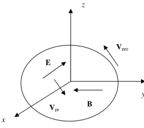
Figure 3 shows the surface perpendicular to the axis OZ , on which the directions of the electric and magnetic fields (32) and the velocities of praons are shown, according to (33). All the vectors correspond to the time point t, at which the condition t 2n is met. The vectors
pr
V and Vpre denote the velocities of the positive and negative praons, respectively.
5. THE PHOTON STRUCTURE
The presence of r in the denominator of the velocity in (23) for the near zone and in (27) for the wave zone leads to decreasing of the velocity amplitude while the distance from the emitting atom is increasing. Obviously, for the photon to exist independently at a certain distance from the atom, the amplitude of the rotation velocity of the negatively charged praons in the photon must stop being dependent on r. By analogy with (20) and (25), in which we will replace r with a certain constant distance z , we will assume the following expressions0
for the amplitude of the electric field inside the photon in the near zone and in the wave zone, respectively:
Fig. 3. The fields (32) and velocities (33) of praons near the axis OZ in the wave zone at t 2n.
z x y E B V pre Vpr
0 1 3 0 0 4 eR E z , 2 0 3 2 0 0 4 e R E z c .
We have an opportunity to estimate the value of z using the data from [14] for the photon0
with the angular frequency 1.54946 10 16 s-1, which emerges in the hydrogen atom in the electron’s transition from the second to the first level in the Lyman series, setting the photon radius equal to R0 4aB. Based on the photon energy and its volume, with equality of the density of this energy and the electromagnetic energy density, we determine the amplitude of
the electric field inside the photon: 6
0 2.1 10
E V/m.
If we equate E and1 E , we obtain0 z0 99aB, where aB is the Bohr radius. However, if we equate E3 and E , then we should obtain0 z0 7aB . In the near zone the field E3 is substantially smaller than the field E , and therefore, only at a small distance from the nucleus1
of the order of 7a , the fieldB E could set the photon’s praons in motion so that it could have3
a field of the order of E . At the boundary between the near and wave zones, which is reflected0
by the condition zc, the value z366aB. Consequently, the internal electromagnetic energy of the photon, associated with the motion of the charged particles in it, appears in it already in the near zone. Here, the particles of the emerging photon are influenced by the electric field (17), consisting of three main components, which get aligned with each other at
z c
and the value z366aB.
The amplitude of the transverse electric field of the second component in (17), according to
(32), at r z z0 is equal to 0 2 2 0 0 4 e R E z c
. From the equality E2 E0 we obtain the
influence on the particles inside the photon than the first component, but its influence is stronger than that of the third field component.
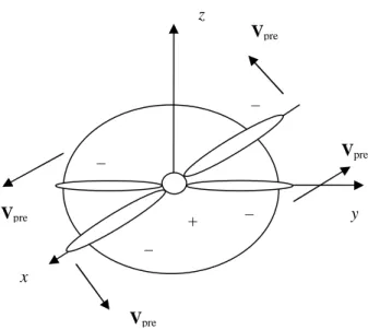
Analyzing the field directions and the velocities of particles in Figures 1-3, resulting from the field components (17), in a first approximation we can develop the photon model, which is
symmetric in its form. The photon’s cross section at t 2n in this model is presented in
Figure 4.
When the rotation phase of the electron in the atom satisfies the relation t 2ntk z, where t is the earlier time point, then for any time point t we can choose such z , with
which the pattern of events will be repeated in the same way as in Figure 4. In this case in Figure 4 the lobes along the axis OX are formed by the negative praons under action of the fields of the form (20) and (25), as in Figures 1 and 2, respectively. In Figure 4, we also added the lobes of the negative praons that are likely to occur under action of the fields (32), as in Figure 3. In the center, near the axis OZ the positive praons are concentrated. The whole
Fig. 4. The photon’s cross section at t 2n. The positive charge near the axis OZ is indicated with , the negative charges of the lobes are indicated with .
Vpre z x y Vpre Vpre Vpre – – + – –