HAL Id: hal-01090484
https://hal.archives-ouvertes.fr/hal-01090484
Submitted on 3 Dec 2014
HAL is a multi-disciplinary open access
archive for the deposit and dissemination of
sci-entific research documents, whether they are
pub-lished or not. The documents may come from
teaching and research institutions in France or
abroad, or from public or private research centers.
L’archive ouverte pluridisciplinaire HAL, est
destinée au dépôt et à la diffusion de documents
scientifiques de niveau recherche, publiés ou non,
émanant des établissements d’enseignement et de
recherche français ou étrangers, des laboratoires
publics ou privés.
Exploiting User Movement for Position Detection
The Dang Huynh, Chung Shue Chen, Siu-Wai Ho
To cite this version:
The Dang Huynh, Chung Shue Chen, Siu-Wai Ho. Exploiting User Movement for Position Detection.
IEEE Consumer Communications and Networking Conference, IEEE, Jan 2015, Las Vegas, United
States. pp.6. �hal-01090484�
Exploiting User Movement for Position Detection
The Dang Huynh
∗, Chung Shue Chen
∗, and Siu-Wai Ho
†∗Alcatel-Lucent Bell Labs, Centre de Villarceaux, 91620 Nozay, France
†Institute for Telecommunications Research, University of South Australia, Australia
Email:{The Dang.Huynh, cs.chen}@alcatel-lucent.com, [email protected]
Abstract—The major issue of indoor localization system is the trade-off between implementation cost and accuracy. A low-cost system which demands only few hardware devices could save the cost but often it turns out to be less reliable. Aiming at improving classical triangulation method that requires several reference points, this paper proposes a new method, called Two-Step Movement (2SM), which requires only one reference point (RP) by exploiting useful information given by the position change of a mobile terminal (MT), or the user movement. This method can minimize the number of reference points required in a localization system or navigation service and reduce system implementation cost. Analytical result shows that the user position can be thus derived and given in simple closed-form expression. Finally, simulation is conducted to demonstrate its effectiveness under noisy environment.
Index Terms—Positioning system, localization algorithm, user movement, mobile device, smart applications.
I. INTRODUCTION
Positioning systems are crucial to today’s digital society. They provide geographic information about devices that facil-itates many human activities. For instance, vehicle navigation systems are indispensable for drivers in big cities. Some location-based services are deployed in commercial malls so that customers can get navigation while walking in complex environment and can receive promotion advertisement from shops. The market of indoor and outdoor location-based ser-vices has grown rapidly in the last decade.
Global positioning system (GPS) is very popular and widely used for user localization. When line-of-sight to at least four GPS satellites is available, location (latitude, longitude, and elevation) and timing information can be obtained. Although GPS is very convenient in outdoors, its quality is susceptible to weather conditions, for example when sky view is poor due to fog, rain, cloud, etc., or being blocked by tall buildings in urban areas. These issues can significantly degrade the accuracy. As expected, GPS is not for indoors due to the lack of line-of-sight. There also exist cellular-based positioning systems [1] which are built on measuring signal strength from three or more base stations for tracking mobile user’s location. However, these solutions also do not work well for indoors.
Various indoor positioning systems have been developed, see e.g., [2]–[4]. They can be categorized into network-based or non-network-based solutions. The network-based approach, which takes advantages of existing network infrastructure such as wireless local area networks (WLANs), without demanding new infrastructure, can maintain low deployment cost. The non-network-based approach uses dedicated positioning
infras-tructure and often can provide higher reliability but with extra cost. For example, solutions based on ultrasound and infrared have high deployment cost. One may also consider simple proximity-based solution like iBeacon [5] which however is only able to offer an approximate location. Some systems consider using visible light to construct an indoor positioning system with high accuracy [6]. A good positioning system should be cost-effective and also be able to offer high accuracy. Constructing an efficient and simple positioning system is always challenging. Technically, it would depend on: 1) the number of available reference points (RPs); 2) the technologies used (e.g., RF-based, ultrasound, infrared, etc.) and; 3) the characteristics of the environment. In this study, we propose a geometry-based positioning method which can determine user position by only using one RP and exploiting user’s simple movement, for instance walking or waving user’s hand-held device, and some simple information. As the solution requires only one RP and can provide either exact result in noiseless environment or accurate positioning in noisy condition, our approach brings competitive advantages compared to other methods, thanks to its simplicity and effectiveness. Meanwhile, the method is interesting and may have a high potential to improve today’s technology or existing solutions.
II. RELATEDWORK
Indoor positioning problem has attracted a lot of interest over years [7], [8]. Studies have been done extensively and many possible solutions have been proposed. There are mainly four major approaches to solve this problem: triangulation, fingerprinting, scene analysis, and proximity.
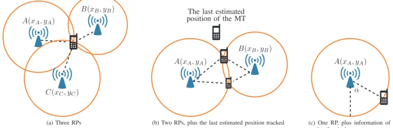
Triangulation is used to estimate the position of a user or mobile terminal (MT) if the geographical coordinates of the RPs are known and assume that the MT is capable of measuring the distance between itself and the RPs. A priori, this method requires three RPs to construct a distinct geometric intersection of three circles, which indicates the position of the MT. The principle is illustrated in Fig. 1(a) (or see e.g., [2]). Note that not all schemes based on triangulation requires three circles (see e.g., Fig. 1(b) and (c)). For instance, given angle-of-arrival (AoA) information, using only one RP is sufficient to locate the MT.
Fingerprinting [9] is to estimate device position by using pre-measured location-related data. This method consists of two phases: an offline training phase and an online position estimation phase. In the offline phase, location-related data is collected at different positions in the area. During the online
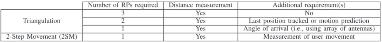
Number of RPs required Distance measurement Additional requirement(s) Triangulation
3 Yes No
2 Yes Last position tracked or motion prediction
1 Yes Angle of arrival (i.e., using array of antennas)
2-Step Movement (2SM) 1 Yes Measurement of user movement
TABLE I: Requirement comparison between triangulation and proposed 2-Step Movement (2SM) method.
position determination phase, real-time location-related data is measured and then matched with the set of data gathered during the offline phase to estimate the device’s location.
Scene analysis[7] is a localization method based on a set of images or scenes received by one or multiple cameras. This approach in principle does not require user (to be tracked) to carry any extra device. However, the solution is usually expensive because it requires one or many cameras to perform tracking and may prone to a high computation cost due to image or video processing.
Proximity detects if a MT is nearby or for example in the coverage area of a RP. However, it is hard to provide accurate position with high reliability.
Each of the above method also has some variants or hybrid schemes. Our proposed geometry-based solution is built on triangulation. We will explain and discuss in comparison other methods stemmed from this branch. The cost and accuracy of triangulation method primarily rely on the number of RPs required. Traditionally, one would need at least three RPs to determine the position of the MT.
Figure 1(b) shows a variant of traditional triangulation method, which requires two RPs and the last estimated previ-ous position of the mobile terminal so as to eliminate one of the two intersection points of the two circles constructed by the two RPs. In such case, the location closer to the last estimated position would be selected. Or, the system has to be able to predict user mobility pattern in order to select one. Note that this method still requires more than one RP. A variant of the above triangulation method is to use only one RP but requires the information of angle-of-arrival (AoA) provided by an array of antennas either implemented in the user terminal (MT) or at the RP [10], see Fig. 1(c). However, such an array of antennas is often costly and cumbersome.
III. SYSTEM DESIGN
Here, we propose a new method called “Two-Step Move-ment (2SM)”. It aims to improve the classical triangulation approach and requires only one RP. It makes use of the changes in the position of the MT relative to the RP. The changes is caused by either active movement (e.g., a user may wave his/her MT to assist) or natural movement (e.g., the user is walking or moving). Therefore, 2SM turns out to have a competitively low deployment cost and without extra or expensive tracking hardware such as antenna array and is able to determine user position in exact closed-form solution. The simplicity and effectiveness would highly facilitate practical indoor positioning systems. Table I gives a comparison of the above methods and outlines their key difference. In our pro-posed 2SM method, the MT is assumed be capable to measure
its movement using its embedded sensors and software.
A. One-Step Movement (1SM)
Our method exploits useful information generated by user movement. For the sake of simplicity, the 2SM is presented as a combination of two One-Step Movements.
One-Step Movement (1SM) relies on one position change (one move) to identify the two possible locations (position candidates) of the MT with the following assumptions:
• The position of the RP is known.
• The MT is capable of measuring the distance between
itself and the RP.
• The MT is capable of measuring the distance and the
angle (direction) of its movement.
Figure 2 illustrates the system design, where
• A is the RP with a known position (xA, yA).
• B is the initial position of the MT that is unknown and
yet to be found. It is denoted by coordinates(xB, yB).
• C is the position of MT right after the first movement,
(xC, yC), which is also unknown.
• MT is capable of measuring the distance between itself
and the RP. That is, the distancesAB and AC are given
for example by measuring the received signal strength or standard techniques.
• MT is capable of measuring the distance and the angle of
its movement, thus BC and the angle α ∈ (0, 2π] (with
respect to the positivex-axis) are also measurable.
Theorem 1 Suppose that A(xA, yA), AB, BC, AC, and α
are known, the One-Step Movement (1SM) will give two estimated locations, denoted by generic point B(xB, yB),
whose x and y coordinates satisfy:
xBcos α + yBsin α = xAcos α + yAsin α
− (AB 2 + BC2 − AC2 ) 2BC . (1)
Proof:Using Fig. 2, from the two measured distancesAB
andAC, the equations of the two circles centered at A(xA, yA)
on which the MT probably lies can be expressed as
(xB− xA)2+ (yB− yA)2 = AB2 (xC− xA)2+ (yC− yA)2 = AC2 (2) where xC = xB+ BC cos α, yC = yB+ BC sin α. (3) From (2), we have AB2 − AC2 = (xB− xC)(xB+ xC− 2xA) +(yB− yC)(yB+ yC− 2yA). (4)
A(xA, yA) B(xB, yB) C(xC, yC) (a) Three RPs A(xA, yA) B(xB, yB)
The last estimated position of the MT
(b) Two RPs, plus the last estimated position tracked
A(xA, yA)
α
(c) One RP, plus information of angle-of-arrival α
Fig. 1: Positioning techniques using different number of reference points (RPs).
SubstitutexC andyC in (3) to (4), we can have
AB2
− AC2
= −BC cos α(2xB+ BC cos α − 2xA)
−BC sin α(2yB+ BC sin α − 2yA)
which can be re-written as
AB2 + BC2 − AC2 = −2BC(xBcos α − xAcos α +yBsin α − yAsin α). Hence,
xBcos α + yBsin α = xAcos α + yAsin α
−(AB 2 + BC2 − AC2 ) 2BC .
We can solve (1) as follows
• If sin α = 0, thus cos α = ±1, (1) becomes:
xB= xA± (AB2 + BC2 − AC2 ) 2BC .
It is then straightforward to compute the values ofxBandyB,
by substituting the value ofxB to (2).
• If sin α 6= 0, by dividing (1) by sin α, we have:
yB = − cot αxB+ xAcot α + yA−
AB2
+ BC2
− AC2
2BC sin α .
Letb = xAcot α + yA− (AB2+ BC2− AC2)/(2BC sin α)
anda = − cot α. We see that now yB can be expressed as a
function of xB such thatyB = axB+ b. Substituting yB to
the first equation of (2), we have
(xB− xA)2+ (axB+ b − yA)2= AB2. Then (1+a2 )x2 B−2xB(xA−a(b−yA))+x 2 A+(b−yA) 2 −AB2 = 0. (5) The above quadratic equation (5) can be solved easily. Algorithm 1 shows in detail how to perform 1SM. It outputs
two points B1(xB1, yB1) and B2(xB2, yB2), which are the
possible solution ofB.
Remark 1 It is clear that one of the two points,B1(xB1, yB1)
and B2(xB2, yB2), must be the position of the MT (or both
of them are, ifB1 and B2 are identical).
x y A(xA, yA) B(xB, yB) C(xC, yC) B(xB, yB) α
Fig. 2: One-Step Movement (1SM).
B. Two-Step Movement (2SM)
After the first movement, we have two possible locations of the MT given by 1SM using Algorithm 1, but cannot determine which one is the true location. We need to resolve this ambiguity. It is natural to think about performing an additional movement. The basic idea is simple: a Two-Step Movement (2SM) is a combination of two consecutive 1SM’s where each move gives two possible positions (in which one of these two positions must be the true position). It is clear that by comparing the results of two 1SM’s, we can determine the location of the MT, given that the results of the two 1SM’s are not redundant.
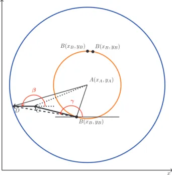
Fig. 3 depicts how 2SM works. The MT makes the second
Algorithm 1 One-Step Movement algorithm
Require: A(xA, yA), AB, AC, BC, α;
1: function ONESTEP(A(xA, yA), AB, AC, BC, α)
2: if sin α == 0 then 3: ifcos α == 1 then 4: xB= xA− (AB 2 + BC2 − AC2 )/(2BC); 5: else 6: xB= xA+ (AB2+ BC2− AC2)/(2BC); 7: end if 8: yB1 = yA+pAB2− (xB− xA)2; 9: yB2 = yA−pAB2− (xB− xA)2; 10: return{B1(xB, yB1), B2(xB, yB2)}; 11: else
12: ⊲ Pre-compute a, b such that yB= axB+ b;
13: a = − cot α; 14: b = xAcot α + yA − (AB2 + BC2 − AC2 )/(2BC sin α); 15: ⊲ Compute xB, yB; 16: ∆ = (xA− a(b − yA))2− (1 + a2)(x2A+ (b − yA)2− AB2); 17: xB1 = (xA− a(b − yA) + √ ∆)/(1 + a2 ); 18: yB1 = axB1+ b; 19: xB2 = (xA− a(b − yA) − √ ∆)/(1 + a2 ); 20: yB2 = axB2+ b; 21: return{B1(xB1, yB1), B2(xB2, yB2)}; 22: end if 23: end function
is measured from the positive x-axis counter-clockwise. The
distanceCD and β are known by the MT, whereas the distance
AD from the MT to the RP is measured from the received signal strength by standard techniques. The underlying idea is that, we now consider the movement of 2SM case similarly
as that of 1SM case in which the starting point is nowB and
the ending point isD. We can compute the distance BD and
the angleγ analytically (see Algorithm 2: line 5–10) and then
use the method of Algorithm 1 to determineB. Algorithm 2
details how 2SM works. By comparing the results from the two 1SM’s computation, we determine the location of the MT. Remark 2 Note that the directions of the two movements
should not be in parallel, i.e.,β 6= α and β 6= α±π, otherwise the ambiguity cannot be resolved since the system of equations generated by the second movement would be equivalent to that of the first one.
In practice with estimation error or system imperfection, say the existence of noise, we may not have a common solution from the two 1SM’s computation. In this case, the first movement may give us two possible solutions denoted
by B1(xB1, yB1) and B2(xB2, yB2), but the second
move-ment may give us another two possible solutions denoted
byB3(xB3, yB3) and B4(xB4, yB4). However {B1, B2} and
{B3, B4} may not have a common point as shown in Fig. 4. To solve this problem, we can choose the pair of points that
x y A(xA, yA) B(xB, yB) C D B(xB, yB) B(xB, yB) γ β
Fig. 3: Two-Step Movement (2SM).
have the smallest distance, i.e., solvingmin{d(P 1, P 2)|P 1 6=
P 2}, for P 1, P 2 ∈ {B1, B2, B3, B4} where d(P 1, P 2)
denotes the Euclidean distance of points P 1 and P 2. After
that, we take their mean (e.g., the mid-point of B1 and B3
in Fig. 4) as the estimate of the MT’s position for minimizing the error. In general, one can formulate it as an optimization problem and find the optimal result.
B2(xB2, yB2) B4(xB4, yB4)
B1(xB1, yB1) B3(xB3, yB3)
Fig. 4: Ambiguity elimination in case of noise.
IV. SIMULATION
Simulation is performed to investigate the performance of the proposed scheme (2SM) under noisy environment. The RP
is placed at the center of a room, i.e.,A = (0, 0). We are going
to determine the MT’s location, denoted byB(xB, yB), which
is randomly distributed in the room. In the following analysis, we consider three distances (1, 5, and 10 meters) between the
MT (denoted byB, in Fig. 3) and the RP. Also, we assume that
the direction fromB to A is uniformly distributed in (0, 2π].
For a givenAB, the movement from B to C or from C to
D is equal to 0.1, 0.2, and 0.5 times of AB. The directions
Algorithm 2 Two-Step Movement algorithm
Require: A(xA, yA);
1: function TWOSTEP(A(xA, yA))
2: MT makes the first movement from B to C; measure AB, AC, BC, α;
3: {B1(xB1, yB1), B2(xB2, yB2)} = ONESTEP(A(xA, yA), AB, AC, BC, α); ⊲ Obtain B1 and B2
4: MT makes the second movement from C to D; measure CD, AD, β; make sure that β 6= α and β 6= α ± π ;
5: X = BC cos α + CD cos β; ⊲ The change in x-coordinate after the second move
6: Y = BC sin α + CD sin β; ⊲ The change in y-coordinate after the second move
7: BD =√X2+ Y2;
8: cos γ = X/BD;
9: sin γ = Y /BD;
10: Compute γ ∈ (0; 2π] from cos γ and sin γ;
11: {B3(xB3, yB3), B4(xB4, yB4)} = ONESTEP(A(xA, yA), AB, AD, BD, γ); ⊲ Obtain B3 and B4
12: B(xB, yB) = {B1(xB1, yB1), B2(xB2, yB2)} ∩ {B3(xB3, yB3), B4(xB4, yB4)}; ⊲ Determine MT location
B(xB, yB) from the set of B1, B2, B3 and B4;
13: return B(xB, yB);
14: end function
(0, 2π]. Estimation error to the measurement of distances AB, AC, AD, and BC, is considered to be bounded in [−1%, 1%],
[−2%, 2%], and [−5%, 5%], for comparison. We use ed to
denote the above bound such that ed = 1%, 2%, and 5%,
respectively. Estimation error to the measurement of angles
α and β is considered to be bounded in [−1◦, 1◦], [−2◦, 2◦],
and[−5◦, 5◦]. The bound on the angle measurement error is
denoted by ea such that ea = 1, 2, and 5 degrees. For each
(ed, ea) setup, the errors are randomly generated to corrupt
the proposed algorithm in determiningB(xB, yB). Results are
shown in Figs. 5, 6, and 7 forBC = CD is equal to 0.1×AB,
0.2 × AB and 0.5 × AB, respectively. Note that each curve in the figures is obtained by 10,000 runs. During these runs, we observe that about 10% of the time the system fails to find the MT position (i.e., the quadratic equation (5) has no solution
since∆ in Algorithm 1 is negative) due to the noise (which
would be accumulated to ∆). We find that when ∆ < 0, the
system is indeed heavily corrupted. In this case, the movement is considered as bad and is not used to locate the MT. Note that it would be interesting to derive the position of the MT
even when∆ < 0 and see how to extract useful information
to optimize results. This is left as future work.
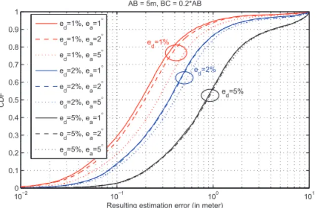
As shown in Figs. 5-7, the estimation error in determining
the position of the MT increases asedincreases. Note that the
estimation error is defined by the distance between the real po-sition of the MT and the result given by Algorithm 2. Clearly,
ed= 1% (curves in “red”) results in smaller estimation error
than thated= 3% or ed= 5% (curves in “blue” and “black”,
respectively) makes, given thatea is the same.
As expected, the estimation error in determining the position
of the MT also increases asea increases. However, whened
is relatively large (5%), the impact of the considered ea is
relatively less significant. This can be clearly shown by Figs. 6
and 7. Roughly speaking,ed is more dominating.
In comparing Figs. 5-7, we observe that when increasing BC and CD from 0.1 × AB to 0.5 × AB, the error in
estimating the position of the MT decreases quite substantially. In Fig. 6 and 7, the curves shift to the left. The distance of the movement is a significant factor. We can improve the system performance by requiring a longer movement distance. However, a longer distance may be less favorable in some scenarios. Furthermore, from the obtained simulation results which are not shown in this paper, we see that the improvement
is indeed decreasing and starts to get flat at 0.5 × AB.
Table II shows the average error in determining the position
of the MT under different AB (at 1, 5, and 10 meters) and
various BC, CD, and noise levels (ed, ea). For AB = 5,
the results are plotted in Figs. 5-7. ForAB = 1 and 10, the
results have characteristics very similar to those in Figs. 5-7 so that they are not shown in this paper. Comparing the
results at AB = 1, 5, and 10, we see that the magnitude of
the error increases roughly proportional toAB. It is clear that
the estimation error is minimized when(ed, ea) are small and
the movement distance is relatively large. Roughly speaking,
ifBC = CD = 0.5 × AB, the performance is quite desirable
fored≤ 2% and ea ≤ 5%. When the movement distance is at
the level of0.2 × AB, the same performance can be achieved
for a smaller ed ≤ 1%. The average error can be limited to
within about 10% of AB. In the best case, the average error
can be less than5% of AB.
V. CONCLUSION
In this paper, we have proposed a new method called Two-Step Movement (2SM) to estimate the position of MT. It requires only one reference point (RP) by exploiting useful information given by the position change of the MT or user movement. One can therefore reduce the number of RPs required and also the system cost. Analytical result shows that the user position can be derived and given in simple closed-form expression with low complexity. Simulation is conducted to study its performance under noisy environment.
It is possible to achieve average error within about 10% of
ed= 1% ed= 1% ed= 1% ed= 2% ed= 2% ed= 2% ed= 5% ed= 5% ed= 5% ea= 1° ea= 2° ea= 5° ea= 1° ea= 2° ea= 5° ea= 1° ea= 2° ea= 5° AB= 1 (BC=CD= 0.1AB) 0.1412 0.1434 0.1581 0.2583 0.2640 0.2708 0.5530 0.5608 0.5691 AB= 1 (BC=CD= 0.2AB) 0.0808 0.0859 0.1036 0.1463 0.1508 0.1631 0.3202 0.3340 0.3417 AB= 1 (BC=CD= 0.5AB) 0.0484 0.0566 0.0896 0.0753 0.0804 0.1086 0.1701 0.1759 0.1868 AB= 5 (BC=CD= 0.1AB) 0.7194 0.7279 0.8027 1.2797 1.3012 1.3668 2.7913 2.9031 2.9226 AB= 5 (BC=CD= 0.2AB) 0.3957 0.4235 0.5513 0.7145 0.7480 0.8246 1.6222 1.6372 1.6587 AB= 5 (BC=CD= 0.5AB) 0.2193 0.2831 0.4481 0.4136 0.4412 0.5448 0.8738 0.8829 0.9134 AB= 10 (BC=CD= 0.1AB) 1.4165 1.4348 1.6130 2.4798 2.6257 2.7011 5.7899 5.8059 5.8929 AB= 10 (BC=CD= 0.2AB) 0.8006 0.8602 1.0845 1.4779 1.1508 1.5112 3.2304 3.3131 3.3873 AB= 10 (BC=CD= 0.5AB) 0.4987 0.5601 0.9362 0.8180 0.8798 0.1058 1.7551 1.7652 1.8750
TABLE II: Average error (in meter) under variousAB, BC, CD, and noise levels (ed, ea).
10−2 10−1 100 101 0 0.1 0.2 0.3 0.4 0.5 0.6 0.7 0.8 0.9 1
Resulting estimation error (in meter)
C D F AB = 5m, BC = 0.1*AB e d=1%, ea=1 ° ed=1%, ea=2° ed=1%, ea=5° e d=2%, ea=1 ° e d=2%, ea=2 ° e d=2%, ea=5 ° e d=5%, ea=1 ° e d=5%, ea=2 ° e d=5%, ea=5 ° e d=2% ed=5% ed=1%
Fig. 5: Resulting error whenAB = 5 meters, BC = CD =
0.1 × AB under various (ed, ea). 10−2 10−1 100 101 0 0.1 0.2 0.3 0.4 0.5 0.6 0.7 0.8 0.9 1
Resulting estimation error (in meter)
C D F AB = 5m, BC = 0.2*AB e d=1%, ea=1 ° ed=1%, ea=2° ed=1%, ea=5° e d=2%, ea=1 ° e d=2%, ea=2 ° e d=2%, ea=5 ° e d=5%, ea=1 ° e d=5%, ea=2 ° e d=5%, ea=5 ° e d=2% e d=5% ed=1%
Fig. 6: Resulting error whenAB = 5 meters, BC = CD =
0.2 × AB under various (ed, ea).
that further analysis of noise impact and issues related to reflection and refraction of signals are important to improve the proposed method. Our method, thanks to the reliance on a single reference point, makes a lot of sense in the context of Internet of Things (IoT) such as home or business office area. It should be also noted that our method can be easily extended to localization in 3D coordinates and to device-to-device (D2D) applications in which both device-to-devices could be mobile. The practical implementation is left as future work.
10−2 10−1 100 101 0 0.1 0.2 0.3 0.4 0.5 0.6 0.7 0.8 0.9 1
Resulting estimation error (in meter)
C D F AB = 5m, BC = 0.5*AB e d=1%, ea=1 ° e d=1%, ea=2 ° ed=1%, ea=5° ed=2%, ea=1° e d=2%, ea=2 ° e d=2%, ea=5 ° e d=5%, ea=1 ° e d=5%, ea=2 ° e d=5%, ea=5 ° e d=1% e d=5% ed=2%
Fig. 7: Resulting error when AB = 5 meters, BC = CD =
0.5 × AB under various (ed, ea).
ACKNOWLEDGMENT
The work presented in this paper has been carried out at LINCS (www.lincs.fr). The authors would like to thank Fabien Mathieu and Philippe Jacquet for their discussion and valuable comments.
REFERENCES
[1] G. Gartner and K. Rehrl, Location Based Services and TeleCartography
II: From Sensor Fusion to Context Models. Lecture Notes in Geoin-formation and Cartography, Springer, 2009.
[2] H. Liu, H. Darabi, P. Banerjee, and J. Liu, “Survey of wireless indoor positioning techniques and systems,” IEEE Trans. Sys. Man Cyber - Part
C, vol. 37, no. 6, pp. 1067–1080, Nov. 2007.
[3] G. Mao, B. Fidan, and B. D. O. Anderson, “Wireless sensor network localization techniques,” Comput. Netw., vol. 51, no. 10, Jul. 2007. [4] A. Kushki, K. N. Plataniotis, and A. N. Venetsanopoulos, WLAN
Positioning Systems: Principles and Applications in Location-Based Services. Cambridge University Press, 2012.
[5] A. Cavallini, iBeacons Bible, http://meetingofideas.files.wordpress.com/ 2013/12/ibeacons-bible-1-0.pdf.
[6] M. Yasir, S.-W. Ho, and B. Vellambi, “Indoor positioning system using visible light and accelerometer,” Journal of Lightwave Technology, vol. 32, pp. 3306–3316, Oct 2014.
[7] Y. Gu, A. Lo, and I. Niemegeers, “A survey of indoor positioning systems for wireless personal networks,” IEEE Commun. Surveys Tuts., vol. 11, no. 1, pp. 13–32, Jan. 2009.
[8] R. Harle, “A survey of indoor inertial positioning systems for pedestri-ans,” IEEE Commun. Surveys Tuts., vol. 15, no. 3, 2013.
[9] P. Mirowski, D. Milioris, P. Whiting, and T. Kam Ho, “Probabilistic radio-frequency fingerprinting and localization on the run,” Bell Labs
Technical Journal, vol. 18, no. 4, pp. 111–133, Feb. 2014.
[10] R. Peng and M. Sichitiu, “Angle of arrival localization for wireless sensor networks,” in IEEE SECON, Sep 2006, pp. 374–382.