HAL Id: hal-02357003
https://hal.archives-ouvertes.fr/hal-02357003
Submitted on 9 Nov 2019HAL is a multi-disciplinary open access
archive for the deposit and dissemination of sci-entific research documents, whether they are pub-lished or not. The documents may come from teaching and research institutions in France or abroad, or from public or private research centers.
L’archive ouverte pluridisciplinaire HAL, est destinée au dépôt et à la diffusion de documents scientifiques de niveau recherche, publiés ou non, émanant des établissements d’enseignement et de recherche français ou étrangers, des laboratoires publics ou privés.
A general and efficient multi-start algorithm for the
detection of loss of ellipticity in elastoplastic structures
Moubine Al Kotob, Christelle Combescure, Matthieu Mazière, Tonya Rose,
Samuel Forest
To cite this version:
Moubine Al Kotob, Christelle Combescure, Matthieu Mazière, Tonya Rose, Samuel Forest. A general and efficient multi-start algorithm for the detection of loss of ellipticity in elastoplastic structures. International Journal for Numerical Methods in Engineering, Wiley, 2019, �10.1002/nme.6247�. �hal-02357003�
DOI: xxx/xxxx
ARTICLE TYPE
A general and efficient multi-start algorithm for the detection of
loss of ellipticity in elastoplastic structures
Moubine Al Kotob
1,2| Christelle Combescure
3| Matthieu Mazière
1| Tonya Rose
2| Samuel Forest*
11Centre des Matériaux, CNRS UMR 7633, MINES ParisTech, PSL Research University, 63-65 rue Henri Auguste Desbruères - BP 87, 91003 Evry Cedex, France
2SAFRAN Paris-Saclay, SAFRAN GROUP, Rue des jeunes bois Châteaufort -CS80112, 78772 Magny-les-Hameaux, France
3Laboratoire Modélisation et Simulation Multi Echelle, MSME, UMR 8208 CNRS, Université Paris-Est, F-77454
Marne-la-Vallée Cedex 2, France
Correspondence
*Samuel FOREST. Email: [email protected]
Summary
The present paper proposes a new efficient and robust algorithm for evaluating the loss of ellipticity criterion. While commonly used in 2D models for thin metal sheet forming processes, it is rarely evaluated in 3D structures due to the computational cost. The proposed algorithm is based on a Newton-Raphson scheme and a multi-sampling optimization method based on a discretization method of the half unit sphere. First the new process is compared to the existing methods in the literature and then it is applied to a structural problem, namely tubes in torsion. The evolution of the loss of ellipticity in these structures is analyzed leading to conclusions about the failure of the structure. Meanwhile, the stability of the discretized problem is ana-lyzed in order to better understand the loss of regularity of the FEM problem. These results are then used to predict the failure of an experimentally tested torsion sample in [1].
KEYWORDS:
Elastoplasticity, Loss of ellipticty, Numerical method, Finite deformation, Strain localization
1
INTRODUCTION
Even though strain localization is one of the most critical phenomena leading to the failure of elasto-plastic structures, its emergence is still not fully understood. Indeed, the term “localization” itself is interpreted differently depending on the context. In a loose sense, localization means the development of high strains in a narrow region of the body, like in a shear band with through thickness necking in a thin plate in tension. A more precise definition is the emergence of strain rate discontinuities through surfaces usually associated with loss of ellipticity, and we use this latter definition in the present work. In some situations, both definitions may even coincide, for instance, a one-dimensional bar displaying a softening behavior experiences simultaneously necking and loss of ellipticity [2], or in thin plates modeled under plane stress conditions [3]. However these definitions do not
MOUBINE AL KOTOB
coincide for 3D models in general. When localization starts in complex structures and whether it leads to catastrophic failure is still an open problem in many situations, especially when certifying industrial components. The example of tubes loaded in torsion [1], shows that even an apparently simple structure can lead to difficulties in defining localization and the localization’s influence on the safety of the global structure.
When dealing with localization, a first distinction needs to be made between types of loss of ellipticity. Strong ellipticity corresponds to definite positiveness of the eigenvalues of the symmetrized acoustic tensor whereas ellipticity refers to the absence of vanishing eigenvalue of the general acoustic tensor [4, 5].
The loss of ellipticity criterion has commonly been adopted as a strain localization criterion. It has been introduced, for instance, in the analysis of the propagation of acceleration waves in [6], as a stability criterion in small deformation in [7], which was then generalized to finite deformations in [8]. According to the latter analysis, in a homogeneously strained domain, a strain localization band can develop when two parallel surfaces fulfill the loss of ellipticity criterion [9], although other local or global instability modes can occur prior to loss of ellipticity in the form of buckling or necking modes. For instance, it is commonly used for the analysis of thin metal sheets forming limits [10] in a plane stress framework. The loss of ellipticity analysis is strictly a local analysis, however, nothing is said about the structural aspect with this criterion. As discussed in [11] around the analysis of localization in polycrystals, loss of ellipticity in a single material element is not enough for the structure itself to fail.
The loss of strong ellipticity criterion is often discussed using a similar approach, especially for geomaterials [12]. Both loss of ellipticity and loss of strong ellipticity can be shown to be equivalent when the tangent operator possesses major symmetry, therefore it is often considered that both conditions are met as long as the material possesses an associative flow rule. However, this is not precisely the case. In some particular cases strong ellipticity and ellipticity will differ in a given finite deformation framework even though the material possesses an associative flow rule [13].
Regarding numerical methods, the evaluation of the loss of ellipticity criterion leads to a minimization problem on one half of the unit sphere where the minimized surface is a sixth order polynomial. Different numerical strategies are available in the literature to solve this minimization problem: Evaluation of the minimum by successive discretization [14], use of a simplex method [15], or definition of an eigenvalue problem [16, 17, 18]. Some strategies combine a Newton-Raphson scheme and a line-search method [19]. The iterative discretization of the half unit sphere is both time consuming and does not ensure the detection of global minimum unless one uses a very fine discretization. Hence, when considering a large structural problem, this strategy would require a large amount of computational power while still not guaranteeing convergence to the global minimum. The simplex method and the eigenvalue problem are standard optimization methods. Given that the global minimum is required and that the minimized surface is a generally non convex sixth order polynomial, it is necessary to take multiple starting points to ensure that the method does not converge to a local minimum. As a consequence, the strategy of coupling Newton-Raphson and line-search methods [19] turns out to be the most promising numerical method. This requires defining a regular discretization
of the half unit sphere, which, usually, is not obtained using a regular discretization of the angles in a spherical coordinates system similar to what is discussed in [20]. Moreover, most methods found in the literature are presented in a small deformation framework [18, 16], and some only for materials possessing an associative flow rule [18].
Finally, it is usually believed that the loss of ellipticity criterion is limited to softening materials and it can be shown that a non-softening material with an associated flow rule can never lead to localization in the sense of Rice within a small deformation framework [21]. This however is not necessarily the case for finite deformations due to the “geometrical” terms. It will be shown in section 4 of this work, that a material that has non-softening behavior can still exhibit localization.
The previous literature review shows that, in spite of many efforts, there is still a need for an efficient and robust strategy to detect loss of ellipticity applicable to structural computations of industrial components. Existing applications are limited to volume elements or mesh subdomains. The objectives of the present work are three-fold: (𝑖) The proposal of an efficient and robust algorithm to detect localization modes; (𝑖𝑖) A failure detection method amenable to the computation of industrial-like samples; (𝑖𝑖𝑖) Interpretation of shear localization modes by means of combined loss of uniqueness and loss of ellipticity criteria. The originality of the work lies in: (𝑖) The robustness and efficiency of the proposed algorithm; (𝑖𝑖) Its use in 3D structural computations; (𝑖𝑖𝑖) Some remarkable observations about the development of the loss of ellipticity domain in a structure under continuing loading. Experimental validation is also provided in the case of a torsion test on a high strength steel used in aeronautics applications. The present work does not consider the post-localization behavior of the structure because the boundary value problem becomes ill-posed as a consequence of loss of ellipticity. Analysis of the post-localization response requires the introduction of regularization methods [22] not included in the present analysis.
In the present work the corotational formulation (hypo-elastoplastic) that is commonly used in most commercial FEM software is presented in section 2.1. In section 2.2, tangent operators, along with loss of ellipticity and loss of strong ellipticity criteria are derived in a closed form. Then, a new general method is presented in section 3 for an efficient evaluation of the loss of ellipticity criterion based on a Newton-Raphson (NR) scheme. While a similar algorithm was introduced in detail in [19], a new initialization method is proposed to improve robustness while being computationally more efficient. This method is derived in the most general case as it does not depend explicitly on the formulation of the constitutive law, and works for both small and finite deformation frameworks. A comparison with the algorithm given in [19] in terms of computation cost is performed on the basic example of a material volume element under simple shear loading at the end of this section. A more complex loading is then presented to underline that the use of multiple starting points improves the robustness of the method leading to a better understanding of the results. In order to illustrate the performance of the method, a structural problem is presented in section 4.1 to evaluate the failure of a tube loaded in torsion. It is shown that while the material is non-softening and possesses an associative flow rule, the loss of ellipticity criterion is met and localization emerges in the simulation. To better understand these results, the loss of uniqueness of the rate boundary value problem is also analyzed and compared to the original localization analysis.
MOUBINE AL KOTOB
Finally, in section 4.2, these latter results will be applied to a real torsion sample used in [1] in order to predict the shear band failure observed in the experiment.
2
RICE’S LOCALIZATION CRITERION
In order to formulate the problem in the most general case, the loss of ellipticity criterion is derived within the finite deformation framework, as in [8].
2.1
Finite deformation formulation
Let 𝑿 be the position of a material point in the reference configuration, Ω0, and 𝒙 (𝑿 , 𝑡) its position in the current configuration, Ω𝑡. The deformation gradient is then:
𝑭∼= 𝜕𝒙 𝜕𝑿 = 𝑰∼+ 𝛁∼𝒖 𝐹𝑖𝑗 = 𝜕𝑥𝑖 𝜕𝑋𝑗 = 𝛿𝑖𝑗+ 𝜕𝑢𝑖 𝜕𝑋𝑗 (1) ̇ 𝑭 ∼= 𝛁∼̇𝒖 𝐹̇𝑖𝑗= 𝜕 ̇𝑢𝑖 𝜕𝑋𝑗 (2) where (⋅) and (⋅)
∼ are first and second order tensors, ∇ is the gradient operator, 𝒖 = 𝒙 − 𝑿 denotes the displacement, ̇𝑎 the time derivative of the quantity 𝑎.
Following Rice’s notation in [8], the Boussinesq stress tensor, noted 𝑺
∼(also called “First Piola Kirchhoff”, or the transposed “Nominal stress tensor”) is given by:
𝑺
∼= 𝝉∼𝑭∼−𝑇 (3)
where J = det(𝑭
∼) denotes the volume ratio, 𝝉∼= J𝝈∼the Kirchhoff stress tensor and 𝝈∼the Cauchy stress tensor. Local equilibrium in the absence of body forces is given by:
𝜕𝑆𝑖𝑗
𝜕𝑋𝑗 = 0 (4)
which gives the following rate form:
d dt (𝜕𝑆 𝑖𝑗 𝜕𝑋𝑗 ) = 𝜕 ̇𝑆𝑖𝑗 𝜕𝑋𝑗 = 0 (5)
2.2
Tangent operators
The developments in section 2.3 require the definition of a tangent operator. For this purpose, the present work is limited to rate constitutive laws that can be expressed as:
̇ 𝑺 ∼=≈ 𝑆 ∶ ̇𝑭 ∼ (6) where ≈ 𝑆
depends on the internal variables and the plastic loading or elastic unloading condition. Equivalently in an updated Lagrangian framework [23] one gets:
̇𝒔
∼=≈ ∶ 𝑳∼ (7)
where 𝑳
∼= ̇𝑭∼𝑭∼−1is the Eulerian velocity gradient, and 𝒔∼is the Boussinesq stress tensor with respect to the current configuration. It is defined as: 𝒔 ∼= 𝝈∼ (8) ̇𝒔 ∼= Tr (𝑳∼)𝝈∼+ ̇𝝈∼− 𝝈∼𝑳∼𝑇 (9) ≈ and≈ 𝑆
can be linked by:
≈ = 1 J(𝑰∼⊠𝑭∼) ∶≈ 𝑆 ∶ (𝑰∼⊠𝑭 ∼ 𝑇 ) (10)
where the “⊠” denotes the dyadic product defined by:
(𝑨∼⊠𝑩
∼)𝑖𝑗𝑘𝑙= 𝐴𝑖𝑘𝐵𝑗𝑙 (11)
While these formulas are general, the expression of
≈ depends on the choice of the finite deformation constitutive law. The
most common laws found in commercial FEM softwares are “hypo-elastoplastic” formulations. Several Eulerian stress tensors can be chosen for this formulation, for instance the Cauchy stress 𝝈
∼, the Kirchhoff stress 𝝉∼, or the Kirchhoff stress in an updated Lagrangian framework ̂𝝉
∼. One can show that the first and third choices are almost equivalent when volume changes are small [23], however, they differ in terms of tangent operator
≈ [13].
Corotational formulation for the Kirchhoff stress
The previous rate constitutive law is now translated into the Jaumann formulation with respect to the Kirchhoff and Cauchy stress tensors because these are formulations widely used in practice, especially in commercial codes. The definition of a
MOUBINE AL KOTOB
corotational formulation of the constitutive law based on the Jaumann derivative of the Kirchhoff stress tensor is given by:
𝝉 ∼ 𝐽 = ≈ 𝜏 ∶ 𝑫∼ (12) with : 𝝉 ∼ 𝐽 = ̇𝝉∼+ 𝝉∼𝛀 ∼− 𝛀∼∼𝝉 (13) where 𝛀 ∼= 𝑳∼ 𝑠𝑘𝑒𝑤 = 1 2(𝑳∼− 𝑳∼ 𝑇 ) and 𝑫∼ = 𝑳∼𝑠𝑦𝑚= 1 2(𝑳∼+ 𝑳∼ 𝑇 ). Then ≈in equation (7) and≈ 𝜏
are linked by:
≈ = 1 𝐽 [ ≈ 𝜏 + 1 2 ( 𝑰 ∼⊠∼𝝉− 𝝉∼⊠𝑰∼− 𝑰∼⊞∼𝝉− 𝝉∼⊞𝑰∼ )] (14)
where “⊞” denotes the dyadic product defined by:
(𝑨∼⊞𝑩
∼)𝑖𝑗𝑘𝑙= 𝐴𝑖𝑙𝐵𝑗𝑘 (15)
In this case, for an associative flow rule,
≈ 𝜏
possesses major and minor symmetries and
≈ major symmetry only. The latter
property leads to the existence of a velocity potential [24]. For this reason, this formulation will be preferred in the present work instead of the following corotational formulation based on the Cauchy stress. It should be noted that the Jaumann formulation may not be the most suitable format to formulate constitutive laws for highly compressible elastoplastic materials like foams [25]. In fact the full constitutive model including hardening laws in particular must be reconsidered for each material for model calibration.
Corotational formulation for the Cauchy stress
The definition of a corotational formulation of the constitutive law based on the Jaumann derivative of the Cauchy stress tensor is given by:
𝝈 ∼𝐽 =≈ 𝜎 ∶ 𝑫∼ (16) with : 𝝈∼𝐽 = ̇𝝈∼+ 𝝈∼𝛀 ∼− 𝛀∼𝝈∼ (17) Then ≈in equation (7) and≈ 𝜎
are linked by:
≈ =≈ 𝜎 +1 2 ( 𝑰 ∼⊠𝝈∼− 𝝈∼⊠𝑰∼− 𝑰∼⊞∼𝝈− 𝝈∼⊞∼𝑰 ) + 𝝈∼⊗𝑰 ∼ (18)
where “⊗” denotes the dyadic product:
(𝑨∼⊗𝑩
∼)𝑖𝑗𝑘𝑙= 𝐴𝑖𝑗𝐵𝑘𝑙 (19)
In this case, for an associative flow rule,
≈ 𝜎
possesses major and minor symmetries and
2.3
Loss of ellipticity and loss of strong ellipticity
Depending on the symmetry of the tangent operator, two material stability criteria are commonly derived, namely loss of ellipticity and loss of strong ellipticity.
Loss of ellipticity
Consider the existence of a surface 𝑆𝑙 in Ω0 with a normal 𝑵 exhibiting a jump of the Lagrangian velocity gradient ̇𝑭∼.
Hadamard’s compatibility condition requires that:
r ̇ 𝑭 ∼ z = 𝒈 ⊗ 𝑵 (20)
where 𝒈 is an unknown vector, andJ⋅Kdenotes the jump of a quantity through the surface 𝑆𝑙. The equilibrium condition on the
stress rates then gives:
r ̇ 𝑺 ∼ z 𝑵 = 𝟎 (21)
Combining equations (6), (20) and (21), and assuming that the tangent operator is the same on both sides of 𝑆𝑙1, one gets:
(𝑵 ⊙
≈ 𝑆
⋅ 𝑵 )𝒈 = 𝟎 (22)
where “⊙” denotes the product2defined by:
(𝒂 ⊙
≈)𝑖𝑗𝑘= 𝑎𝑙𝑖𝑙𝑗𝑘 (23)
𝑵 ⊙
≈ 𝑆
⋅ 𝑵 is the acoustic tensor.
Knowing that the material is initially elastic, and therefore det(𝑵 ⊙
≈ 𝑆
⋅𝑵 ) is initially strictly positive, equation (22) is satisfied as soon as:
det(𝑵 ⊙
≈ 𝑆
⋅ 𝑵 ) = 0 (24)
This condition can be reformulated in the current configuration by using Nanson’s formula given in equation (25):
𝒏 ds = J𝑭∼−𝑇𝑵 dS (25)
1Both sides fulfill the plastic loading condition.
2This notation is unnecessary in a small deformation framework since the tangent operator possesses minor symmetries, nor is it necessary when using the nominal stress tensor 𝑵∼= 𝑺∼𝑇, then𝑁
𝑗𝑖𝑘𝑙= 𝑆 𝑖𝑗𝑘𝑙.
MOUBINE AL KOTOB
where 𝑵 is the unit normal to dS, a surface element in the reference configuration; and 𝒏 is the unit normal to ds, the same surface element in the current configuration. Combining equations (24) and (25) gives the equivalent Eulerian condition (26):
det(𝒏 ⊙
≈⋅ 𝒏 ) = 0 (26)
Note that while the following equations are derived within a Lagrangian framework, equation (26) is the one solved to get the normal in the current configuration, the one that will be observed in reality.
Loss of strong ellipticity
A similar criterion can be formulated starting from the positive definiteness of the second order work which is given by:
̇ 𝑺
∼∶ ̇𝑭∼>0 ∀ ̇𝑭∼= 𝒈 ⊗ 𝑵 (27)
This condition is violated when
det((𝑵 ⊙
≈ 𝑆
⋅ 𝑵 )𝑠𝑦𝑚) = 0 (28)
where (𝑨
∼)𝑠𝑦𝑚denotes the symmetric part of the tensor 𝑨∼. This is the loss of strong ellipticity criterion. Note that equations (24) and (28) are equivalent when
≈ 𝑆
possesses major symmetry.
3
GENERAL ALGORITHM FOR NUMERICAL DETECTION OF LOSS OF ELLIPTICITY
In an FEM framework, the evaluation of the loss of ellipticity criterion is reduced to the solution of a minimization problem after the global convergence of each load increment at each Gauss point of the mesh. Since solving so many minimization problems can be very expensive, it is important to establish an efficient method. In addition, it is necessary to ensure that the global minimum is found in order to properly evaluate this criterion.3.1
Minimization problem
As shown in section 2.3, the loss of ellipticity criterion is formulated in terms of vanishing eigenvalues of the acoustic tensor that depends on a normal 𝑵 .
∃𝑵 , ‖𝑵 ‖ = 1 ∶ det(𝑵 ⊙
≈ 𝑆
As discussed in [16, 19, 26], since
≈ 𝑆
is initially the elasticity tensor3, it is sufficient to evaluate the sign of the smallest determinant and check if:
min ‖𝑵‖=1 ( det(𝑵 ⊙ ≈ 𝑆 ⋅ 𝑵 ))≤ 0 (30)
Formulated in a Cartesian coordinate system, this is a three-dimensional minimization problem with constraint. In order to reduce the size of the system, one can choose a spherical coordinate system such that the constraint on the norm of 𝑵 is automatically fulfilled: 𝑵({𝜽} ) = ⎛ ⎜ ⎜ ⎜ ⎜ ⎜ ⎜ ⎜ ⎜ ⎜ ⎜ ⎜ ⎝ cos(𝜃1) sin(𝜃2) sin(𝜃1) sin(𝜃2) cos(𝜃2) ⎞ ⎟ ⎟ ⎟ ⎟ ⎟ ⎟ ⎟ ⎟ ⎟ ⎟ ⎟ ⎠ with {𝜽} = ⎧ ⎪ ⎪ ⎪ ⎨ ⎪ ⎪ ⎪ ⎩ 𝜃1 𝜃2 ⎫ ⎪ ⎪ ⎪ ⎬ ⎪ ⎪ ⎪ ⎭ (31)
FIGURE 1 On the left, the spherical coordinate system; On the right, det(𝒏 ⊙
≈⋅𝒏 ) surface plotted after stereographic projection
in the (𝑂, 𝒆
𝑧,𝒆𝑥) plane for an elastoplastic shear problem.
The problem (30) then becomes:
min {𝜽} ( det(𝑵 ⊙ ≈ 𝑆 ⋅ 𝑵 ))≤ 0 (32)
3The fourth order tensor of elastic moduli is definite positive. Then det(𝑵 ⊙ ≈
𝑆
MOUBINE AL KOTOB
Note that 𝑵 ⊙
≈ 𝑆
⋅ 𝑵 is an even expression of 𝑵 . Therefore, it is not necessary to analyze the whole unit sphere, but only one half of it. This leads to:
𝜃1 ∈ [0; 𝜋[ , 𝜃2 ∈ [0; 𝜋[ (33)
This leads to a two-dimensional minimization problem:
𝜕det(𝑵 ⊙ ≈ 𝑆 ⋅ 𝑵 ) 𝜕𝜃𝑖 = 0 𝑖= 1, 2 (34)
Using the chain rule, one gets:
⎧ ⎪ ⎨ ⎪ ⎩ 𝝏 det(𝑵 ⊙ ≈ 𝑺 ⋅ 𝑵 ) 𝝏𝑵 ⎫ ⎪ ⎬ ⎪ ⎭ 𝑇 ⋅ [𝝏𝑵 𝝏{𝜽} ] = {𝟎} (35) where 𝜕(det(𝑵 ⊙ ≈ 𝑆 ⋅ 𝑵 )) 𝜕𝑁𝑝 =[det(𝑵 ⊙ ≈ 𝑆 ⋅ 𝑵 )](𝑵 ⊙ ≈ 𝑆 ⋅ 𝑵 )−1𝑗𝑖 (𝑆 𝑖𝑝𝑗𝑙+ 𝑆 𝑖𝑙𝑗𝑝)𝑁𝑙 (36) and [𝝏𝑵 𝝏{𝜽} ] = ⎡ ⎢ ⎢ ⎢ ⎢ ⎢ ⎢ ⎢ ⎢ ⎢ ⎢ ⎢ ⎣
− sin(𝜃1) sin(𝜃2) cos(𝜃1) cos(𝜃2)
cos(𝜃1) sin(𝜃2) sin(𝜃1) cos(𝜃2)
0 − sin(𝜃2) ⎤ ⎥ ⎥ ⎥ ⎥ ⎥ ⎥ ⎥ ⎥ ⎥ ⎥ ⎥ ⎦ (37)
To simplify the coming derivations, the following notations are introduced:
(𝑪∼)𝑝𝑙 = (𝑵 ⊙ ≈ 𝑆 ⋅ 𝑵 )−1𝑗𝑖 (𝑆 𝑖𝑝𝑗𝑙+ 𝑆 𝑖𝑙𝑗𝑝) (38) 𝑨 = 𝜕(det(𝑵 ⊙ ≈ 𝑆 ⋅ 𝑵 )) 𝜕𝑵 = det(𝑵 ⊙≈ 𝑆 ⋅ 𝑵 )𝑪∼⋅ 𝑵 (39) {𝒂} ={𝑨} 𝑇[ 𝝏𝑵 𝝏{𝜽} ] = ⎧ ⎪ ⎨ ⎪ ⎩ 𝝏(𝐝𝐞𝐭(𝑵 ⊙ ≈ 𝑺 ⋅ 𝑵 )) 𝝏{𝜽} ⎫ ⎪ ⎬ ⎪ ⎭ (40)
3.2
Numerical minimization algorithm
Solving equation (35) leads to the evaluation of extrema or saddle points. Some optimization methods, like the gradient method, avoid maxima by always taking a descent direction. Others, like a standard Newton Raphson (NR) method, provide a quadratic convergence, but only search for a vanishing gradient and therefore can include maxima. Thus, in order to capture a
minimum, one needs to initialize the algorithm close to the solution [19]. However, this requires performing some expensive computations to select a “good starting point” and even this is not sufficient to ensure the evaluation of the global minimum4.
In this paper, we propose to reduce the initialization flaw by setting multiple starting points in section 3.2.3.
3.2.1
Sphere discretization for starting points
First, setting multiple starting points means discretizing the half unit sphere. Previous approaches [16, 17, 19, 26] are based on a regular discretization of the Euler angle space. However this method does not provide a strictly isotropic distribution in all directions, as discussed in [20] for composites and [27] in the context of fatigue life assessment. In order to have a uniform discretization and avoid clustering at the poles, only 𝜃2is regularly discretized. For a given discretization parameter 𝑛𝜃
2∈ ℕ, 𝑛𝜃2
regularly spaced points are taken in]0, 𝜋[. Then, in order to discretize 𝜃1, for a given 𝜃2(that defines a circle on the unit sphere, see Figure 1 ) 𝛿𝜃1is computed in order to keep a constant surface element:
FIGURE 2 In red dots, discretization obtained for constant surface element discretization; in blue dots, discretization obtained
for regular angular discretization. On the left, 𝑛𝜃
2= 5; on the right, 𝑛𝜃2 = 36. Top, sphere seen from top; bottom, global view.
MOUBINE AL KOTOB 𝛿𝜃2= 𝜋 𝑛𝜃 2 (41) 𝛿𝜃1(𝜃2) = 𝛿𝜃2 | sin(𝜃2)| (42)
Finally, to avoid singularities when 𝜃2= 0[𝜋], a single point at the pole is added separately to the discretization.
Implementation remark:we take 𝑛𝜃
1= <
𝜋
𝛿𝜃1 >(where “<⋅ >” denotes the integer part), then 𝛿𝜃1is recomputed as 𝜋 𝑛𝜃
1
. As shown in Figure 2 , this method has the advantage of providing an isotropic distribution as well as reducing the number of discretization points5.
3.2.2
Newton-Raphson scheme
This section mainly aims to introduce the expression of the necessary Hessian matrix and the related notations for the imple-mentation of the NR algorithm. Computation of this matrix requires sub-factors that have already been computed along the process beforehand, in section 3.1.
Given a starting point {𝜽}𝑘, an increment {𝚫𝜽}𝑘+1is searched such that:
{𝒂
({𝜽}𝒌+ {𝚫𝜽}𝒌+𝟏)} = {𝟎} (43)
Considering a linear extrapolation with reference to {𝜽}𝑘, next increment {𝚫𝜽}𝑘+1is obtained by solving:
{𝚫𝜽}𝑘+1 = −[𝒉({𝜽}𝒌)]−1⋅{𝒂({𝜽}𝒌)} (44) [ 𝒉({𝜽}𝒌)] = 𝜕 {𝒂 ({𝜽}𝒌)} 𝜕{𝜽} (45)
where [𝒉] denotes the Hessian matrix. Usually this method is avoided in minimization methodologies, because it can have two major flaws:
1. One cannot ensure convergence to a minimum depending on the starting point and the convexity properties of the problem; in our case, this would be a major flaw;
2. Computation and inversion of the second derivative (Hessian matrix) can be very expensive depending on the size of the problem.
While the first flaw cannot be avoided with a simple NR scheme6, other than by taking multiple starting points, the second flaw
is of no concern in our case. The problem to solve for each iteration is two-dimensional: The Hessian matrix is a 2 × 2 matrix
5In fact, the number of points tends to 2
𝜋𝑛
2
𝜃2for constant surface element discretization, when angular discretization has 𝑛
2points. 6In order to overcome this difficulty, the NR scheme is coupled with a line-search in [19].
which is easy to invert. In addition, most of the Hessian matrix’s terms have already been computed while evaluating the gradient of det(𝑵 ⊙
≈ 𝑆
⋅ 𝑵 ) (see equations (38), (39) and (40)). In fact, the second derivative ([𝒉] ) is given by:
[𝒉] = {𝒂}⋅ {𝒂} 𝑇 det(𝑵 ⊙ ≈ 𝑆 ⋅ 𝑵 )+ [𝜼] + det(𝑵 ⊙≈ 𝑆 ⋅ 𝑵 ) [𝝏𝑵 𝝏{𝜽} ]𝑇[ 𝑪 ∼− (𝑻𝑩∼∶ 𝑩∼ 𝑻)] [ 𝝏𝑵 𝝏{𝜽} ] (46) 𝜂𝛼𝛽= 𝐴𝑖 𝜕2𝑁 𝑖 𝜕𝜃𝛼𝜕𝜃𝛽 (47) [ 𝜕 𝜕𝜃1 (𝜕𝑁 𝑖 𝜕𝜃𝛼 )] = ⎡ ⎢ ⎢ ⎢ ⎢ ⎢ ⎢ ⎢ ⎢ ⎢ ⎢ ⎢ ⎣
− cos(𝜃1) sin(𝜃2) − sin(𝜃1) cos(𝜃2)
− sin(𝜃1) sin(𝜃2) cos(𝜃1) cos(𝜃2)
0 0 ⎤ ⎥ ⎥ ⎥ ⎥ ⎥ ⎥ ⎥ ⎥ ⎥ ⎥ ⎥ ⎦ and [ 𝜕 𝜕𝜃2 (𝜕𝑁 𝑖 𝜕𝜃𝛼 )] = ⎡ ⎢ ⎢ ⎢ ⎢ ⎢ ⎢ ⎢ ⎢ ⎢ ⎢ ⎢ ⎣
− sin(𝜃1) cos(𝜃2) − cos(𝜃1) sin(𝜃2)
cos(𝜃1) cos(𝜃2) − sin(𝜃1) sin(𝜃2)
0 − cos(𝜃2) ⎤ ⎥ ⎥ ⎥ ⎥ ⎥ ⎥ ⎥ ⎥ ⎥ ⎥ ⎥ ⎦ (48) where 𝐵𝑗𝑝𝑠 = 𝐵𝑠𝑝𝑗 = (𝑵 ⊙ ≈ 𝑆 ⋅ 𝑵 )−1 𝑠𝑖( 𝑆 𝑖𝑝𝑗𝑙+ 𝑆
𝑖𝑙𝑗𝑝)𝑁𝑙is the only quantity that has to be computed (other terms are given in
equations (38), (39) and (40)).
Implementation remark:Given such expressions, from a numerical point of view, an efficient evaluation of the tensor/matrix products is necessary to limit computation cost. In fact, these terms are not necessarily expensive to evaluate since they can be evaluated in a direct computation: there are no conditionals to evaluate and all factors can be directly computed. For some programming languages, likeC++, the use of “inline” functions is recommended. This remark is of the utmost importance in the performances given later in this paper.
3.2.3
Initialization and general scheme
A multi-point initialization scheme is necessary to ensure the evaluation of the global minimum. Fortunately, the sixth order polynomial surfaces are very smooth7, see Figure 1 , so for any “good starting point” a basic NR scheme converges in very
few iterations (4 to 5 for a tolerance of 10−8on the gradient’s norm). Therefore, in the scheme presented in Figure 3 , multiple starting points are considered while keeping a low number of iterations for the NR Scheme.
Yet, it is important to note that this algorithm captures both minima and maxima. The determinant of the Hessian matrix would inform us about the nature of the extremum. It is however computationally expensive and does not help to reach the global minimum. Instead, several starting points are considered. By taking enough starting points, the smallest solution found
7det(𝑵 ⊙ ≈
𝑆
MOUBINE AL KOTOB
FIGURE 3 Proposed minimization algorithm.
should capture the global minimum. A discretization parameter 𝑛𝜃
2 = 5 (cf. section 3.2.1) has been found to be sufficient for the
isotropic materials considered in the present work. Using up to 6 or 7 is expected to be enough for anisotropic materials. The algorithm is validated with a simple shear loading test using a finite deformation framework. Performance and robustness are shown with comparison to the method proposed in [19] on a more complex loading condition.
3.3
Validation
A shear loading case is studied in order to validate the method on a reference case. The simulation is run on a single Gauss point, and loading is prescribed through the deformation gradient:
𝑭
∼= 0.2𝑡(𝒆𝑥⊗𝒆𝑦+ 𝒆𝑦⊗𝒆𝑥) + 𝑰∼ (49)
where 𝑡 is the fictitious time (loading parameter). The parameter 𝑛𝜃
2 is fixed to 6. For this simulation, a material characterized
FIGURE 4 Simple shear: localization band with normals 𝒆𝑥and 𝒆
𝑦
by a von Mises yield function is adopted and formulated within the corotational framework using the Kirchhoff stress tensor, with nonlinear isotropic hardening. The yield function 𝑓 and the plastic flow rule are given by:
𝑓(𝝉∼, 𝑅) = √ 3 2∼𝝉 𝑑𝑒𝑣∶ 𝝉 ∼𝑑𝑒𝑣− 𝑅(𝑝) (50) 𝑫∼𝑝= ̇𝑝𝜕𝑓 𝜕𝝉 ∼ = ̇𝑝𝑷∼ (51)
where 𝑝 denotes the cumulative plastic strain, and 𝑅(𝑝) the yield stress.
The hypoelastic law, the Young modulus, the Poisson ratio and the isotropic hardening for our simulations are respectively given by: 𝝉 ∼𝐽 = 𝚲≈ ∶ (𝑫∼− 𝑫∼ 𝑝 ) (52) 𝐸= 200 GPa, 𝜈= 0.33 (53) 𝑅(𝑝) = 1000 + 100(1 − 𝑒−300𝑝) − 700𝑝 (54) where 𝝉 ∼𝑑𝑒𝑣= 𝝉∼− Tr (𝝉 ∼)
3 ∼𝑰denotes the deviatoric part of the Kirchhoff stress tensor, and 𝚲≈ is the isotropic fourth order elasticity
tensor. The function 𝑅(𝑝), expressed in MPa, defines the current yield stress and accounts for nonlinear isotropic hardening. The Jaumann derivative is used in the hypoelastic relation (52). Replacing the Jaumann derivative by another objective derivative like Green-Naghdi’s derivative would lead to a different constitutive law. However, in the present case of ductile metals, the elastic strains remain small. Numerical simulations using both derivatives lead to the same response for the torsion loading considered in the validation section, so that essentially the same localization behavior is expected. Finally, combining equations (50) to (52) gives: ≈ 𝜏 = 𝚲 ≈− ⎧ ⎪ ⎪ ⎪ ⎨ ⎪ ⎪ ⎪ ⎩ 0 if 𝑷∼∶ 𝚲 ≈ ∶ 𝑫∼ <0 ( 𝑷∼∶𝚲 ≈ ) ⊗(𝚲 ≈∶𝑷∼ ) 𝐻+𝑷 ∼∶𝚲≈∶𝑷∼ if 𝑷 ∼∶ 𝚲≈ ∶ 𝑫∼ ≥0 (55) where 𝐻 = 𝑑𝑅
𝑑𝑝 is the hardening modulus. Within a small deformation framework, it is known, for such loading and material
FIGURE 5 Surface det(𝑵 ⊙
≈ 𝑆
⋅ 𝑵 ) plotted after stereographic projection in the (0, 𝒆
𝑧,𝒆𝑥) plane for visualization purposes.
The red dots indicate the 3 solutions of the minimization problem at various load increments. All three solutions for shear loading are captured by the algorithm.
MOUBINE AL KOTOB
[3], that the loss of ellipticity criterion is first fulfilled when:
𝐻 = 0; 𝒏 = 𝒆
𝑥or 𝒏 = 𝒆𝑦 (56)
see Figure 4 for the definition of axes. In this case, it occurs for 𝑝 = log(300
7 )∕300 ≃ 0.0125. Since strains are very small
before loss of ellipticity, the results given in equation (56) are valid even in a finite deformation framework. Numerical results are shown in Figures 5 and 6 . Three solutions are equivalently obtained: ±𝒆
𝑥and 𝒆𝑦. 0.0000 0.0025 0.0050 0.0075 0.0100 0.0125 0.0150 0.0175 p 0.00 0.25 0.50 0.75 1.00 R R0 H H0 det(nLn) det(nEn)
loss of ellipticity
0.00 0.01 p −1.0 −0.5 0.0 0.5 1.0n
x 0.00 0.01 p −1.0 −0.5 0.0 0.5 1.0n
y 0.00 0.01 p −1.0 −0.5 0.0 0.5 1.0n
zFIGURE 6 On top, the evolution of the hardening modulus (𝐻) and the minimum of det(𝒏 ⊙
≈⋅ 𝒏 ); both vanish for 𝑝 = 0.0125.
On bottom, the component of the normal minimizing det(𝒏 ⊙
≈ ⋅ 𝒏 ); two solutions are found: ±𝒆𝑥and 𝒆𝑦(𝒆𝑥and −𝒆𝑥are
equivalent solutions). One can remark that both solutions are equivalently obtained while min(det(𝒏 ⊙
≈⋅ 𝒏 )) evolves smoothly.
3.4
Performance and robustness
In the previous section, robustness with respect to the existence of two equivalent minima has been illustrated for the proposed algorithm (see Figures 5 and 6 ). In the following example, the proposed method is compared with another method from the
literature in terms of performance and robustness when there exist multiple local minima associated to different normals 𝒏 but only one single global minimum.
FIGURE 7 Left, The surface det(𝒏 ⊙
≈⋅𝒏 ) is plotted after stereographic projection in the (0, 𝒆𝑧,𝒆𝑥) plane in the elastic regime
(left) and in the plastic regime (right). Red dots denote the solutions obtained with the proposed algorithm; white triangles indicate the solutions obtained using the sampling method.
As discussed in detail in [28], the methods available in the literature propose a two-step process: first, a sampling over the unit sphere (unit cube for the method proposed in [28]) is performed to choose a starting point close to the minimum; then, a minimization algorithm is applied. To do this, many authors propose to discretize the sphere, by regularly discretizing the spherical angles [16, 17, 19, 26].
In this section, it is shown that this two step process is not robust enough to always capture the global minimum. The com-parison is made between: 𝑛𝜃
2= 6 (cf. section 3.2.1) as the discretization parameter of the proposed method; and for the angular
discretization of the spherical angles 𝑛 = 36 to be consistent with the methods proposed in the literature (“every 5𝑜”)8. Using
these parameters leads to almost equivalent computation time for both algorithms: the proposed method being faster by 10% for
𝑛𝜃
2= 6 and 40% for 𝑛𝜃2= 5.
In the following example the material properties are given by:
𝐸= 20 GPa, 𝜈= 0.33 (57)
𝑅(𝑝) = 1000 + 100(1 − 𝑒−25𝑝) − 300𝑝 (58)
The simulation is run on a single material point, and loading is prescribed through the deformation gradient:
𝑭
∼ = 𝑰∼+ 0.075𝑡𝒆𝑥⊗𝒆𝑦+ 0.225𝑡𝒆𝑦⊗𝒆𝑥 (59)
MOUBINE AL KOTOB 0.00 0.02 0.04 0.06 0.08 p 0.00 0.25 0.50 0.75 1.00 det (nLn ) musti-start sampling 0.070 0.075 0.080 0.085 0.090 p −0.006 −0.004 −0.002 0.000 0.002 0.004 0.006 multi-start sampling 0.000 0.025 0.050 0.075 p −1.0 −0.5 0.0 0.5 1.0 n x nx 0.000 0.025 0.050 0.075 p −1.0 −0.5 0.0 0.5 1.0 n y ny 0.000 0.025 0.050 0.075 p −1.0 −0.5 0.0 0.5 1.0 nz nz
FIGURE 8 Comparison between the proposed method based on multiple initialization (multi-start) and the method available
in the literature based on sampling (sampling): a) evolution of min(det(𝒏 ⊙
≈⋅ 𝒏 )) for the different algorithms; b) Zoom of a)
around loss of ellipticity; c), d) and e) components of arg min(det(𝒏 ⊙
≈⋅ 𝒏 )) for the different algorithms. Results differ in the
plastic regime where two local minima exist.
Numerical results are shown in Figures 7 and 8 . The proposed method with multiple initialization points is denoted “multi-start” and the method based on sampling is denoted “sampling”. The solution is the same for both methods in the elastic regime (existence of a unique global minimum), but the results differ in the plastic regime (existence of two local minima with slightly different amplitudes). Not only do they lead to different loadings at loss of ellipticity, but also to very different normal vectors. Only the mult-start method captured the global minimum. Thus, the proposed method is found to be more robust than the algorithms available in the literature for capturing the global minimum. The simulation with the loading condition (59) which exhibits no special symmetry property proves that the existence of multiple local minima with different critical strains at loss of ellipticity and distinct band orientations is a general feature of finite elatoplasticity. This underlines the importance of a multi-start algorithm to avoid attraction by a single well. This is illustrated here in the case of isotropic von Mises plasticity but is expected for more general anisotropic yield criteria.
4
APPLICATION TO A TUBE LOADED IN TORSION
In order to demonstrate the efficiency and robustness of the proposed algorithm when applied to a structure, two examples are given in this section. Some fundamental results given in [29] about the uniqueness of the solution are illustrated. The imple-mentation of the proposed algorithm and the simulations are performed in theZsetsoftware (http://www.zset-software.com/) environment [30].
4.1
Application to a simple tube
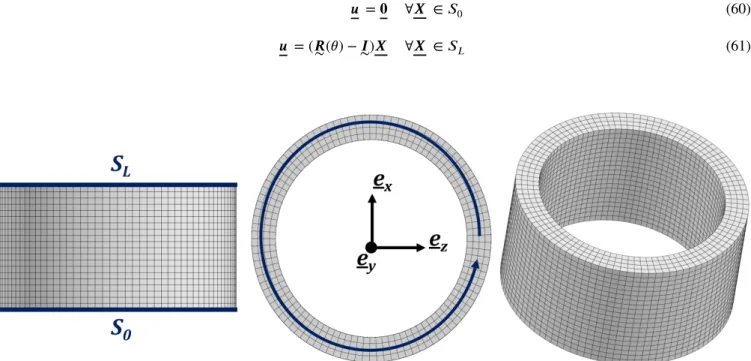
A tube of external diameter 𝐷 = 1 𝑚𝑚, thickness 𝑡 = 0.1 𝑚𝑚 and length 𝐿 = 0.5 𝑚𝑚 is loaded in torsion. The tube is oriented along the (𝑂, 𝒆
𝑦) axis and its lower and upper surfaces are respectively denoted 𝑆0and 𝑆𝐿, as shown in Figure 9 . On the bottom
surface 𝑆0, all displacements are fixed; on the top surface 𝑆𝐿, displacements are imposed to describe a rotation as follows:
𝒖 = 𝟎 ∀𝑿 ∈ 𝑆0 (60)
𝒖 = (𝑹∼(𝜃) − 𝑰∼)𝑿 ∀𝑿 ∈ 𝑆𝐿 (61)
FIGURE 9 Geometry and boundary conditions. 𝑆0is fixed in all directions, a rotation around (𝑂, 𝒆
𝑦) is prescribed to the nodes
on 𝑆𝐿.
An exponential hardening material is described by a corotational formulation for the Kirchhoff stress tensor (see section 2.2) endowed with a von Mises yield function such that:
𝐸= 200 GPa, 𝜈= 0.33 (62) 𝑓(𝝉∼, 𝑅) = √ 3 2∼𝝉 𝑑𝑒𝑣∶ 𝝉 ∼𝑑𝑒𝑣− (1000 + 300(1 − 𝑒−5000𝑝)) (63)
MOUBINE AL KOTOB
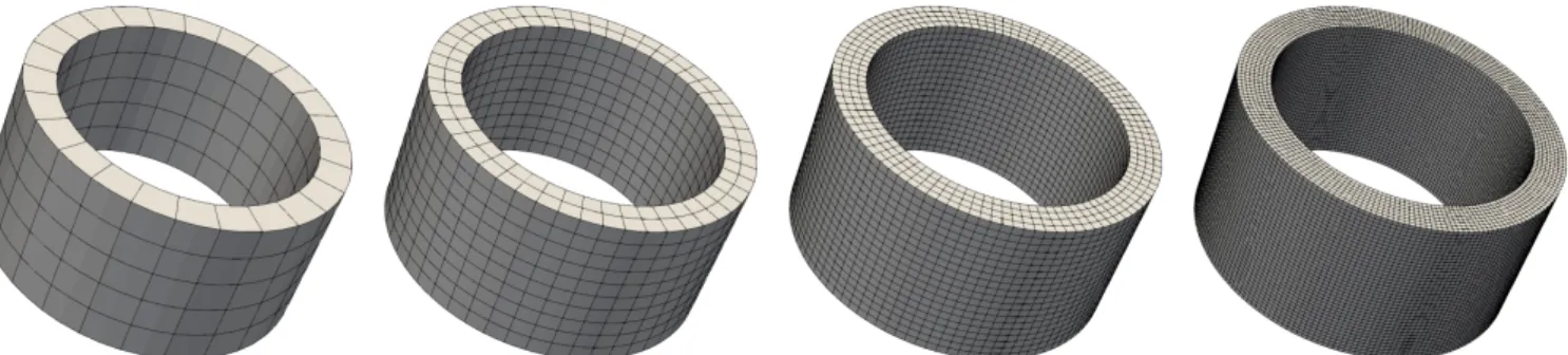
Four mesh refinements will be studied, see Figure 10 . They are made of regular hexahedral elements with 20 nodes, 27 integra-tion points, i.e. quadratic interpolaintegra-tion and full integraintegra-tion. This element type is chosen to avoid hourglass modes and locking behavior. For large isochoric plastic deformations it is more usual to resort to reduced integration instead of full integration in order to limit checkerboard effect of the hydrostatic stress. However, this effect is not significant in the presented torsion simulations at limited strain levels.
FIGURE 10 From left to right, meshes are numbered from 1 to 4: 125 (ℎ = 0.1 𝑚𝑚), 1000 (ℎ = 0.05 𝑚𝑚), 8080 (ℎ = 0.025 𝑚𝑚),
64320 (ℎ = 0.0125 𝑚𝑚) quadratic elements (20 nodes, 27 Gauss points).
4.1.1
Swift effect
In the following simulations, no defect is introduced in the mesh to trigger localization. However, since all displacements are imposed on 𝑆0and 𝑆𝐿the solution naturally displays some gradient along the longitudinal direction as shown in Figure 11 . This is known as the “Swift effect” when simulating a simple torsion test on a tube at finite deformation [31]. Localization occurs in the middle section of the tube as a consequence of this non-homogeneous field. Such concentration in the middle section can be observed in some experimental setups in [1, 32].
4.1.2
Evolution of loss of ellipticity
The evolution of loss of ellipticity in the thickness of the tube is presented in this section. Numerical results are given in Figure 12 for the second coarsest mesh of Figure 10 :2 elements through the thickness, 10 along the length and 50 around the circumference. The computation using the proposed minimization algorithm lasts 324 𝑠 for 100 load increments9: 119 𝜇𝑠 per
Gauss point per increment with 𝑛𝜃
2= 5.
The tube is initially elastic and the solution of the minimization problem is constant and positive with 𝒏 = ±(√2∕2𝒆
𝜃−
√
2∕2𝒆𝑦). When 𝜃 = 0.45𝑜, plasticity starts on the outer skin of the tube, ±𝒆
𝜃 and ±𝒆𝑦 become equivalent minimizers of
FIGURE 11 Plot of the longitudinal stress 𝜎𝑦𝑦in MPa in the tube at 𝜃 = 0.01𝑜.
FIGURE 12 From left to right and top to bottom: Evolution of accumulated plastic strain and min(det(𝑵 ⊙
≈ 𝑆
⋅ 𝑵 )) in the lower half of the tube for 𝜃 ={0.12𝑜,0.45𝑜,0.81𝑜,0.89𝑜,0.8935𝑜,0.8975𝑜,0.94875𝑜,1.0𝑜}. The solution of the minimization
problem is plotted with rods colored by the amplitude of the minimum obtained with the proposed method in each Gauss point; red indicates loss of ellipticity. For visualization purposes, not all Gauss points are represented on these plots.
MOUBINE AL KOTOB
det(𝑵 ⊙
≈ 𝑆
⋅ 𝑵 ). Ellipticity is first lost on the outer-skin when 𝜃 = 0.81𝑜. Then, plastic strain quickly increases in the middle
section once the loss of ellipticity reaches the inner-skin (𝜃 > 0.8975𝑜). This occurs in the middle section of the tube due to
the longitudinal compression and tension stresses (cf. Figure 11 ). In fact, the strain localization in the middle section can be observed in some experimental setups [32]. Finally, once localization starts in the middle section of the tube, the rest of the structure elastically unloads.
As presented in section 2.3, the loss of ellipticity criterion (det(𝒏 ⊙
≈⋅ 𝒏 )≤ 0) is linked to the emergence of jumps in strain
rates across a surface of normal 𝒏 . In the present case (shear), both 𝒆
𝜃and 𝒆𝑦are directions that fulfill the latter criterion. Due
to the robustness of the minimization algorithm both solutions are captured. The jumps in strain rates occur through a surface of normal 𝒆
𝑦(the surface is a transverse section of the tube). If only one solution was obtained by the minimization algorithm, for
example 𝒆
𝜃, it might not be possible to link the emergence of the localization bands with a normal 𝒆𝑦to the loss of ellipticity
criterion. Thus, this example highlights the utmost importance for the algorithm to be robust with respect to the existence of multiple equivalent minima.
4.1.3
Mesh and time-stepping sensitivity
In this section one of the main characteristics of loss of ellipticity is observed, namely the sensitivity of the results with respect to mesh and time step sizes. For this purpose, four meshes are investigated (shown in Figure 10 ). From coarsest to finest, meshes are numbered from 1 to 4.
The evolution of accumulated plastic strain and min(det(𝑵 ⊙
≈ 𝑆
⋅ 𝑵 )) in the lower half of the tube depending on the mesh size is described by the Figures 13 and 14 . No mesh dependence of the torque-angle curves is observed before ellipticity is lost through the whole thickness of the tube. This interval between first occurrence of loss of ellipticity and the spreading of this zone through the thickness is visible on the curves of Figure 14 . After this critical point, the thickness and location of bands depend on the specific mesh size. A rigorous size of localized zones cannot be properly defined. When localization occurs, there exist multiple modes leading to various band widths. However, the smallest localization band possible is defined by the Gauss point size. Thin bands with half an element thickness are visible in Figure 13 (mesh 3 for instance) and also in Figure 15 (mesh 2). The mesh size only slightly influences the rate of decrease of the torque in Figure 14
Structured meshes only are considered in the present work, see Figure 10 . Mesh dependence is also expected with respect to the shape and orientation of finite elements. Regular, oriented and random meshes have been compared in [33] and shown to lead to very different post-localization patterns. For the sake of brevity, such an investigation is not untaken here.
The time-step sensitivity of the results is illustrated by Figures 15 and 16 . For given mesh size, the effect of time step refine-ment remains small except that larger plastic strain values are found in some localization bands. The effect of time discretization
on the torque-angle curves is visible once ellipticity is lost through the whole thickness. These effects can be further interpreted by performing an additional analysis related to loss of uniqueness, as done in the next section 4.1.4.
FIGURE 13 From left to right and top to bottom: Evolution of accumulated plastic strain and min(det(𝑵 ⊙
≈ 𝑆
⋅ 𝑵 )) in the lower half of the tube for models 1 to 4 at 𝜃 = 1𝑜. The solution of the minimization problem is plotted with rods colored by
the amplitude of the minimum obtained in each Gauss point; red indicates loss of ellipticity. For visualization purposes not all Gauss points are represented on these plots.
4.1.4
Loss of uniqueness of the FEM problem
In an infinite functional space, uniqueness of the rate boundary value problem is lost as soon as det(𝒏 ⊙
≈ ⋅ 𝒏 ) < 0 for at
least one 𝒏 in an arbitrary small area. However, in a discretized problem such instability modes cannot necessarily emerge due to the kinematics imposed by the shape functions defined in the elements. In the present example it will be shown that the loss of uniqueness of the discretized problem occurs only once ellipticity is lost in a region crossing the whole thickness of the tube. It is known that the uniqueness of the rate boundary value problem is lost as soon as the smallest eigenvalue of the global stiffness matrix becomes negative [8, 29, 34, 5, 35]. Therefore, in order to analyze the uniqueness of the computed solution, the smallest eigenvalues of the global stiffness matrix of the FEM problem have been extracted. It is shown in Figure 17 that all eigenvalues are positive for 𝜃 ≤ 0.89𝑜and nine eigenvalues become negative for the next step 𝜃 = 0.9𝑜, which corresponds to
the loading step for which ellipticity is lost through the whole thickness of the tube.
The part of the structure in which ellipticity is lost before localization occurs has a finite thickness regardless of the mesh size, as shown in Figure 18 . This leads to the existence of multiple localization bands of various thicknesses, infinitely many in an infinite functional space, but limited by the number of layers of elements in a FEM model. The number of instability modes is
MOUBINE AL KOTOB 0.0 0.2 0.4 0.6 0.8 1.0
θ[
o]
0 20 40 60 80 100 T orque [N.mm]first loss of ellipticity
loss of ellipticity through thickness h = 0.1 mm h = 0.05 mm h = 0.025 mm h = 0.0125 mm 0.80 0.85 0.90 0.95 1.00 95.870 95.875 95.880 95.885 0.875 0.900 0.925 0.950 0.975 1.000
θ[
o]
0.003 0.004 0.005 +9.588×101FIGURE 14 Torsion test: On the left, torques obtained for the different mesh sizes (h); on the right, zoom at maximum torque
(𝜃 ∈ [0.8, 1.0]).
FIGURE 15 Results in terms of accumulated plastic strain and loss of ellipticity for 𝜃 = 1𝑜, using mesh of model 2. Top, constant
load-steps (0.01𝑜); bottom, refined load-steps. For the same loading and same mesh, results differ in terms of plastic strain: The
first case has a maximum plastic strain of 𝑝𝑚𝑎𝑥= 0.011, and the second case has a maximum plastic strain of 𝑝𝑚𝑎𝑥= 0.015 due
0.0 0.2 0.4 0.6 0.8 1.0
θ[
o]
0 20 40 60 80 100 T orque [N.mm]first loss of ellipticity
loss of ellipticity through thickness constant time steps
small time steps
0.80 0.85 0.90 0.95 1.00 95.870 95.875 95.880 95.885 0.875 0.900 0.925 0.950 0.975 1.000
θ[
o]
0.003 0.004 0.005 +9.588×101FIGURE 16 Torsion test: On the left, torques obtained for constant and refined time-steps; on the right, zoom at maximum
torque (𝜃 ∈ [0.8, 1.0]) 0.0 0.2 0.4 0.6 0.8 1.0 −0.5 0.0 0.5 1.0
λ
min ≤ 0 λ0 λ1 λ2 λ3 λ4 λ5 λ6 λ7 λ8 λ9 0.86 0.87 0.88 0.89 0.90 0.91 0.92 0.93θ [
o]
−0.2 −0.1 0.0 0.1λ
min ≤ 0λ0 λ1 λ2 λ3 λ4 λ5 λ6 λ7 λ8 λ9FIGURE 17 Evolution of the ten smallest eigenvalues of the global stiffness matrix. Nine eigenvalues become negative as soon
MOUBINE AL KOTOB
FIGURE 18 Sign of the det(𝒏 ⊙
≈⋅ 𝒏 ) in the tube loaded in torsion at 𝜃 = 0.9 𝑜.
FIGURE 19 Eigen-modes associated to the nine vanishing eigenvalues from Figure 17 at 𝜃 = 0.9𝑜for the torsion of a tube
consistent with the number of Gauss point layers that are contained in the non-elliptic zone of Figure 18 . Finally, the instability modes form a basis for all possible localization bands in the sense of Rice that could emerge in the FEM problem, as shown in Figure 19 .
As proposed in [29], once a “disk-like” zone in which ellipticity is lost has fully developed, localization in the sense of Rice (bands) occurs10. In fact, loss of ellipticity in a single Gauss point is not enough for the FEM model to fail [29], yet it is an
indicator of a weak, most likely critical, zone in the structure [36].
Another fundamental result is observed. Once localization in the sense of Rice occurs, the rest of the structure elasti-cally unloads [13, 3, 2]. This usually leads to a sudden drop in the structure’s stiffness, yet shear has almost zero geometric consequences in terms of effective cross–section. Therefore, this leads to a slightly decreasing torque [2] (cf. Figure 14 ).
4.2
Application to an experimental torsion sample
In this section the analysis of loss of ellipticity is applied to a real torsion sample in order to detect a shear localization band. The geometry and mesh are shown in Figure 20 . The experimental results using this sample are taken in [1].
FIGURE 20 Geometry of the torsion sample. A regular mesh (quadratic interpolation) is used in the gauge length. Flat surfaces
are cut on the sample’s heads in order to apply the torsion load.
This sample has been loaded in torsion, and exhibits, for the material properties given in [1], a localization band in the gauge length due to loss of ellipticity. These results are shown in Figures 21 to 23 .
It is shown that the sample has the same kind of behavior regarding the evolution of loss of ellipticity as the simple tube studied in section 4. Yet, a difference can be observed due to the sample’s geometry. The flat surfaces added to the heads for testing purposes break the axial symmetry. This leads to the existence of two zones where elastic unloading occurs later. In fine, the plastic strain localized in a narrow band. As it can be seen in Figures 21 and 22 , the applied torque keeps on increasing after the first loss of ellipticity. Once ellipticity is lost through the thickness of the middle section and once there is elastic unloading in the rest of the gauge length, the maximum torque is reached. Then, although the material is non-softening, the applied torque
10In [29], the author also discusses some geometrical compatibility with the boundary conditions, which is met in this case: The rotation of the upper surface is consistent with the shear band in the middle section.
MOUBINE AL KOTOB 0 2 4 6 8 10 12 14 θ [o] 200 400 600 800 1000 1200 1400 Ty D π (R 4 e− R 4 i) [M P a ] 1 234 5 6 no loss of ellipticity loss of ellipticity Maximum Experiment FEM
FIGURE 21 Evolution of normalized torque as a function of the loading angle for the whole loading process. Comparison
between FEM simulation and experimental results. 𝑇 denotes the torque, 𝐷 the external diameter, 𝑅𝑒and 𝑅𝑖, the external and internal radii, and 𝜃 the torsion angle in degrees. In squares, the instants shown in Figure 23 ; the red triangle shows the maximum torque. 6.5 7.0 7.5 8.0 8.5 9.0 9.5 θ [o] 1380 1385 1390 1395 1400 1405 1410 1415 1420 Ty D π (R 4 e− R 4 i) [M P a ] 2 3 4 5 6 no loss of ellipticity loss of ellipticity Maximum Experiment FEM
FIGURE 22 Evolution of torques as a function of the loading angle zoom around the localization point. Comparison
FEM/experiment. In squares, the instants shown in Figure 23 ; the red triangle shows the maximum torque.
decreases. Such localization bands were observed experimentally in [1]. It is shown in Figures 21 and 22 that the numerical results correlate well with the experimental observations.
FIGURE 23 From left to right, top to bottom: Evolution of loss of ellipticity and cumulative plastic strain in the gauge length
of the sample. The solution of the minimization problem at each Gauss point is plotted in rods; red rods for loss of ellipticity.
5
CONCLUSIONS
A new general algorithm based on a Newton-Raphson scheme is proposed for evaluating the loss of ellipticity criterion. It is derived in the most general case and it does not depend explicitly on the formulation or on the associativity of the plastic flow. This algorithm has been shown to be more robust and more efficient than methods available in the literature. In order to reach maximal efficiency, a method to discretize the unit sphere has been proposed, which has the twin benefits of providing an isotropic distribution as well as reducing the number of discretization points. This proposed multi-start method has been compared to the classical sampling method found in the literature[19]. It is shown to be more robust when multiple minima exist while requiring a shorter computation time than other methods. The existence of multiple local minima was found to be generic for the various investigated loading conditions.
The new method was applied in a structural FEM problem to evaluate the failure of a tube loaded in torsion. It has been shown that, while the material of the tube is non-softening and possesses an associative flow, the loss of ellipticity criterion is
MOUBINE AL KOTOB
met and localization emerges in the simulation. Also, the use of the multi-start algorithm proposed in this paper, which is robust when there are multiple equivalent global minima, allowed both solutions to be captured and properly interpret the results in section 4. The last application on a complex torsion sample shows that this method of failure detection is amenable to industrial applications in spite of the demanding computational effort associated with nonlinear minimization algorithms.
The use of loss of ellipticity criterion can be advantageously combined with conditions for loss of uniqueness in order to gain more insight on the emergence of localization modes and interpret the observations made in section 4. It was shown in section 4.1.4 that the instability modes were as numerous as the number of possible localization bands (in the sense of Rice) that could kinematically emerge in the non-elliptic domain of the FE mesh. This links to the fact that kinematically admissible fields are restricted by the FEM shape functions and such localization modes were observed only once ellipticity was lost through the whole thickness of the tube. This is an interesting outcome of the proposed study which requires further work especially regarding the use of finer and finer mesh sizes allowing for fine structured localization modes.
As a conclusion, the originality of the work is three-fold: (𝑖) An efficient and robust algorithm to detect localization modes was presented; (𝑖𝑖) The failure detection method is amenable to the computation of industrial-like samples in contrast to existing applications that are limited to volume elements or mesh subdomains; (𝑖𝑖𝑖) The observed shear localization modes are interpreted by means of combined loss of uniqueness and loss of ellipticity criteria showing that loss of ellipticity through the whole thickness of the tube is required for full localization to occur.
It has been observed in a structural problem that loss of ellipticity in a part of the structure in an FEM problem is not enough for the discretized problem to lose regularity. In fact, localized shear bands appear in the tube only once ellipticity has been lost through the whole thickness of the tube. Also, the cross–section in which loss of ellipticity occurs is parallel to the surfaces of application of the boundary conditions, and the normals minimizing det(𝒏 ⊙
≈ ⋅ 𝒏 ) are perpendicular to that surface. All
together, these conditions allow the emergence of shear strain localization bands. Finally, this method has been applied to a real torsion sample used in [1] to detect the emergence of a localization bands during a torsion test.
Non-proportional loading can occur in structural components so that the difference between isotropic and kinematic hardening can result in distinct localization behavior. This can be investigated within the proposed method. Some elements of localization analysis at finite elastoplastic deformation using isotropic and kinematic hardening have been provided in [37]. This constitutive feature was not considered in the present work which concentrates on validation examples for high strength steels displaying little hardening so that the differences resulting from the use of isotropic or kinematic models are expected to be small. Exten-sions of the present work towards the analysis of curvature surface effects will require the consideration of isotropic/kinematic hardenings.
The simulations presented in this work do not show strain levels larger than 0.1. However the full finite deformation framework is needed for loss of ellipticity to occur in materials displaying hardening or perfect plasticity. The post-localization behavior was
not considered in the work due to the loss of regularity of the solution. Regularization methods are required for the simulation of the post-localization structural response, for instance using strain gradient plasticity at large deformations [22]. The presented algorithm is used here to detect loss of ellipticity in order to know when to stop the computation. The engineering applications mentioned in the paper deal with high strength steels that are prone to shear band localization after a small amount of strain. The method can be applied efficiently to predict the onset of failure in components made of such alloys.
References
1. Defaisse C., Mazière M., Marcin L., Besson J.. Ductile fracture of an ultra-high strength steel under low to moderate stress triaxiality. Engineering Fracture Mechanics. 2018;194:301–318.
2. Jirásek M.. Mathematical analysis of strain localization. Revue Europeenne de Genie Civil. 2007;11:977–991.
3. Besson J., Cailletaud G., Chaboche J.-L., Forest S.. Non-linear mechanics of materials. Springer; 2010.
4. Petryk H.. Material Instabilities in Elastic and Plastic Solids. In: CISM International Centre for Mechanical Sciences 414. 2000;.
5. Bigoni Davide. Nonlinear Solid Mechanics: Bifurcation Theory and Material Instability. Cambridge University Press; 2012.
6. Hill R.. Acceleration waves in solids. Journal of the Mechanics and Physics of Solids. 1962;10:1–16.
7. Mandel J.. Conditions de Stabilité et Postulat de Drucker. In: Rheology and Soil Mechanics IUTAM Symposium Grenoble: 58–68; 1966.
8. Rice J.R.. The localization of plastic deformation. In: Theoretical and Applied Mechanics:207–220 North Publishing Company; 1976; Philadelphia.
9. de Borst R., Wells G.N., Sluys L.J.. Some observations on embedded discontinuity models. Engineering Computations. 2001;18:241–254.
10. Ben-Bettaieb M., Abed-Meraim F.. Effect of kinematic hardening on localized necking in substrate supported metal layers.
International Journal of Mechanical Sciences.2017;123:177–197.
11. Abed-Meraim F.. Contributions à la prédiction d’instabilités de type structure et matériau : modélisation de critères et formulation d’éléments finis adaptés à la simulation des structures minces. Mémoire HDR dissertation Arts et Métiers ParisTech 2009.