HAL Id: hal-00626175
https://hal.archives-ouvertes.fr/hal-00626175
Submitted on 23 Sep 2011HAL is a multi-disciplinary open access archive for the deposit and dissemination of sci-entific research documents, whether they are pub-lished or not. The documents may come from teaching and research institutions in France or abroad, or from public or private research centers.
L’archive ouverte pluridisciplinaire HAL, est destinée au dépôt et à la diffusion de documents scientifiques de niveau recherche, publiés ou non, émanant des établissements d’enseignement et de recherche français ou étrangers, des laboratoires publics ou privés.
A plot drainage network as a conceptual tool for the
spatial representation of surface flow pathways in
agricultural catchments
Pierre Aurousseau, Chantal Gascuel-Odoux, Hervé Squividant, Ronan Trépos,
Florent Tortrat, Marie-Odile Cordier
To cite this version:
Pierre Aurousseau, Chantal Gascuel-Odoux, Hervé Squividant, Ronan Trépos, Florent Tortrat, et al.. A plot drainage network as a conceptual tool for the spatial representation of surface flow pathways in agricultural catchments. Computers & Geosciences, Elsevier, 2009, 35, pp.276-288. �hal-00626175�
Elsevier Editorial System(tm) for Computers & Geosciences Manuscript Draft
Manuscript Number: CAGEO-D-07-00056R1
Title: A plot drainage network as a conceptual tool for the spatial representation of surface flow pathways in agricultural catchments
Article Type: Original Paper
Keywords: GIS; DEM; drainage network; tree structure; graph structure; agricultural catchment. Corresponding Author: Chantal Gascuel-Odoux,
Corresponding Author's Institution: INRA, Agrocampus Rennes, UMR 1069, Sol Agronomie Spatialisation First Author: Pierre Aurousseau
Order of Authors: Pierre Aurousseau; chantal Gascuel-Odoux; Hervé Squividant; Forent Tortrat; Ronan Trepos; Marie-Odile Cordier
Abstract: The drainage network must take the farming systems and the landscape structure into
consideration to describe flow pathways in the agricultural catchment. A new approach is proposed to build the drainage network which is based on the identification of the inlets and outlets for surface water flow on each farmers' field (or plot), estimating the relative areas contributing to the surface yield. The delineation of these areas and their links in terms of surface flow pathways provides us with a pattern of relationships between individual plots, i.e. going from each plot to the other plots over the entire catchment. In this approach, flow directions are firstly calculated in the usual way by taking account of slope direction. Plot outlets are defined from the DEM then linked together using a tree structure. If present, linear networks such as hedges modify both the flow directions and the location of plot outlets, hence modify this tree structure. In a final step, the plots are themselves linked together using a graph structure illustrated by an arrow diagram. This drainage network based on plot outlets is applied to a 15-km² catchment area represented by 38,300 pixels and 2,000 plots. This new drainage network takes into consideration 5,300 plot outlets, which greatly reduces the number of objects in comparison with a drainage network made up of pixels or DEM cells. This method leads to a simple and functional representation of surface flow pathways in an agricultural
pathways are coming from numerous or large-sized plots. Finally it produces a functional representation for decision support.
General comment
If a new review is required by the editor, we would like that the opinion of a third reviewer would be required, due to the completely opposite opinion of the two present reviewers. We can also suggest to get the opinion of a specialist in spatial analysis (such as A. Mc Bratney, Heuvelink,…) better than an hydrologist. Coupling this new spatial method with a
hydrological model is not the focus of this paper despite it has been realized otherwise. The focus of the paper is to present a method for representing the spatial structure of rural catchments regarding to the surface flow pathways. This method is interesting by itself, with or without including it in a hydrological modelling.
Response to the first reviewer
(1) I am nor sure that word 'spatialisation' is widely used by hydrologists. I think it might be better to replace it by 'representation' or 'representation of the spatial distribution'
(2) Abstract line 3 'these' not 'them' (3) Abstract line 10 'modify' not 'modified' (4) Page 2 line 27 'small-sized'
(5) Page 3 line 4 replace 'are' by 'being a' (6) Page 3 line 7 'based on'
(7) Page 4 line 5 'a plot' not 'as plot'
(8) Page 4 lines 15 and 16. replace 'allow to get a' by 'permits the establishment of a' (9) Page 4 line 19 'strips'
(10) Page 5 line 19 'In'
(11) Page 6 line 6 'by Tortrat (2005)'
(12) Line 9 Please define 'bocage' for non-French readers (13) Page 10 line 18 'research in an operational mode'
(14) Page 10 lines 19 and 20 'thus affecting material transport' (15) Page 11 line 7 'poorly suited'
(16) Page 11 line 13 insert 'and' after 'processed'
(17) Page 13 line 15 replace 'hydric erosion of soils' by 'water erosion' or 'erosion of soils by water' Response : All these minor errors have been corrected.
Reviewer #2:
1.Is this a new and original contribution?
A comparison with classical methods needs to be conducted in order to show the originality of the method.
Response:
The first two lines of the abstract and the key words have been modified: the hydrological modelling is no more the objective of the paper. The words model or modelling have been removed and replaced by “spatial representation”or discretization of the catchment (p. 1, l7, l16, l27; p.2, l6, l25; p.3 l6, l20) Coupling a transfer model in the discussion (§4.2 added)
Thus the paper is focused on a functional spatial representation of surface flow over the catchment. And, thus the contribution on the spatial representation of a rural catchment is completely original. And, thus, the comparison with the classical modelling approaches can not be addressed. The different way for the spatial representation of a catchment is more developed in introduction (p.2 l10 to l19; p.3 l7 to l8) Additional figures (Fig. 9 and 10) have been added to illustrate the interest in getting a
functional description of the catchment by this original method, and described in the text (p. 10, l19 to l28).The discussion on the interest of this original method has been extended in the discussion (§4.1 extended).
New arguments have been added on the interest of this method for future (p. 13, l20 to p. 14 l6) 2. Is the paper of interest to geoscientists, mathematicians, computer scientists, statisticians, or general?
Not, in its present form. The paper should include a comparison of the novel method to classical ones, and a demonstration of hydro-chemical modeling benefit through an application case.
Response : Coupling a transport model have been realized otherwise and submitted in an other paper. Nevertheless, the discussion treats this point in a new specific paragraph and discuss about the interest and limitations for coupling transport processes.
3. Are the conclusions and interpretations valid?
The paper lacks of a convincing application case illustrating the domain of application of the method and how it can be used in modeling water and pollutant transfer.
Response: see above.
5. Are the illustrations pertinent? Yes but not sufficient
Response: two illustrations have been added to convince of the interest of getting such a spatial representation of the catchment.
7. Can the text or illustrations be condensed? Yes
The paper is very short presenting and illustrating the method in14 pages with a double space interline.
9. Is the abstract informative?
Yes. However, the two first lines deal with pollution transfer while the paper doesn't present any application case.
Response: these first two lines have been removed. 10. Are the references adequate?
The references need to be completed by adding well-known references on channel network extraction (see for example O'Callaghan and Marks, 1984; Band, 1986 Water Resour. Res.; Montgomery and Dietrich, 1989, Water Resour. Res.; etc.).
Response: they have been added. Moreover it is detailed where these classical methods have be used (p. 5, l21 to l25), and where original methods have been developed (p. 6, l8 to l12; p.7, l24)
General comments :
The paper aims to present a methodology to spatialize surface flow pathways taking into account the plot plan structure. A GIS-procedure is developed using Digital Elevation Models, channel network location and plot limits. An application case is given on a 15 km² watershed. As stated by the authors, this approach can be used for "distributed models to understand and predict non-point source pollution in agricultural catchments". This topic is of international interest. However, the paper lacks of
soundness, a justification in comparison to the state of the art, and a clear application case of the modeling approach. The paper should include a comparison of the novel method to classical ones, and
a demonstration of hydro-chemical modeling benefit through an application case. My major comments concern:
First : The paper presents an application case to extract and to identify a connectivity matrix of the treelike drainage network using a grid based Digital Elevation Models crossed with the plot limits. However, the paper doesn't present any application case to show how this spatial discretization can be used neither in distributed hydrological modeling, neither for non-point source pollution transfer as announced in the objectives. Generally, the watershed spatial discretization is conducted function of the structure of the hydrological model, the hydrological and hydro-chemical processes modeled, and the connectivity between surface, subsurface and aquifer flows. The paper doesn't state clearly, how the modeler can use the results of the study, and for what range of models and applications this discretization can be useful. Is this procedure adapted for existing grid-based models (i.e. the SHE model)? If not, what will be the constraints to develop a hydrological model
that takes into account this surface discretization (Does the model exist or needs to be developed? How to proceed?). What applications can this procedure be used for? An application case for hydro-chemical modeling should be conducted to demonstrate the domain of application of the procedure. Response
We deliberately chose in this article to present only the spatial representation of the surface flow pathways for several reasons: (1) this representation requires sufficient space and it would have been difficult in space assigned to present this spatial representation simultaneously and satisfactorily with its use in a hydrological model, (2) the authors chose to present the hydrological transfer model dedicated for pesticide transport and coupled to this spatial representation (presented in an international conference and cited in reference: Cordier et al., 2005), (3) the spatial representation can be used for itself while it makes possible to highlight the portions of the catchment which do not contribute to feed the stream network by surface runoff (page 10, l. 4-6), those which contribute to it and the nodal points of the catchment where an obstacle to the surface transfer is particularly relevant to stop feeding the stream network (page 10, l. 8-12).
Thus, following the remark of this reviewer we decided to develop the use of the spatial representation for itself in this article, and to indicate that the insertion of this spatial model is possible in any hydrological model and already realized in one pesticide transfer model.
The reviewer requests also if this spatial representation can be adapted to existing models based on regular grids such as the SHE model. The answer to this question is positive but all the answers require a necessary adaptation since in a model with a grid system such as the SHE model, water is routed from cell to cell whereas in the model we developed, surface flow routing from cell to cell is replaced by contributive area to contributive area surface flow routing. Infiltration flow can be represented similarly per plot or part of plot, or stay per pixel as presently in the SHE model.
Second : The paper doesn't present clearly the originality of the approach in comparison to well known method used in GIS to extract the drainage network from DEMs (see for example O'Callaghan and Marks, 1984; Band, 1986 Water Resour. Res.; Montgomery and Dietrich, 1989, Water Resour. Res.; etc.). What will be the difference between the method presented herein, and a classical method which i) identifies sub-watersheds from DEM, and than ii) subdivide each watershed using the plot limits. A comparison between classical methods and the new one should be undertaken.
Response
The spatial representation presented in this article does not aim to replace traditional techniques of DEM treatment. The reviewer quotes two examples of classical DEM treatment:
(1) Locating the stream network. This technique is not implemented since the true stream network, including the network of ditches, is initially introduced in a vector data base then imported in the raster data base by a procedure of rasterisation (page 5, l. 4).
(2) Extraction of subcatchments. We did not carry out this extraction in our procedure. And the contours of studied catchments were extracted by the traditional procedure from DEM treatment before the use of our spatial method.
(3) The originality of our method is in the addition of the classical procedure which aggregates the pixels according to a functional schema which consist in building a plot outlet tree and plot tree structure. Thus, following this remark of this reviewer it is now clearly indicated that the originality does not consist in the basic treatment of the DEM but in a following and new further step which consists in the aggregation of the pixels according to functional units which are here the plot or a part of plot feeding a plot outlet, then the plot outlet tree and the plot tree.
Third : I'm not convinced that the use of a regular grid (herein 20 x 20 m) is well adapted to represent linear plot limits and ditches : for example plots limits or ditches have 0.1 to 2 m width (for example) while the spatial representation of the procedure presented herein is a set of square pixels of 400 m²! The authors must clarify for what kind of hydrological processes the discretization can be used, and how to represent surface flows on the identified units. What will be the uncertainty on the model results due to this approximation ?
Response:
The reviewer is right when he recalls that the plot limits and ditches have a width from 0,1 to 2 m whereas the spatial representation proposed here is based on pixels of 20 X 20 m, that is to say 400 m². But this question is largely beyond the purpose of this article and it is quite clear that distributed hydrological models have to evolve towards the use of multi-resolution data bases or variable resolution data bases. Some of the authors of our article who practise the techniques and software of the field of virtual reality know the technical solutions of spatial description by use of multi-resolution or variable resolution data bases : for example the techniques of the Levels Of Details (LOD) and of Active Surface Description (ASD). But their use in distributed hydrological models stay complex while the easy use of regular grid models imposes its law up to now including in topographic data bases. Hydrologists are expecting the production, marketing and diffusion of topographic data bases with variable resolution where the resolution evolves/moves according to topography - what is the base of the technique of the Levels of Details. It would constitute a first stage to evolve the distributed hydrological models towards a spatial description based on variable resolution.
To reconsider in a more detailed and explicit way the use of a regular grid structure to the upstream of our spatial representation, one can reconsider two types of objects where this question of resolution deserves discussion.
- Concerning the stream and ditches network, the role of these networks are important: taking them into account seems essential even with the detriment of their real width.
- Concerning plot limits and hedges, the solution we proposed to circumvent - in a way that seems to us skilful - the question of their width since what we call the « wall » function which is at the base of the redirection of the flow drainage directions is ensured by an object without width, since this « wall » function is provided by the edge of the hedge pixels which are at the edge of the plot.
Consequently, the choices we made as well concerning the stream network cells as the hedge cells do not deny the constraints imposed by the use of regular grid based models. The original solution for « hedges » pixels can be implemented in any spatial schema.
Fourth : The paper deals with linear networks such as ditches and hedges. How about other spatial elements? How these linear elements can be represented in a hydrological model? How to represent hydro-chemical processes on these elements? The identification of these linear elements, and the connectivity must be done function of the hydro-chemical processes to be modeled, and function of the space and time steps of input variables (rainfall, watertable, soil and landuse maps, etc.) : For example for hourly or daily time step input data, do we really need such a spatial discretization. The paper doesn't also present clearly the domain of application of the procedure : i.e. How to deal with flat areas? What are the limitation function of the grid size?
Response:
The linear objects such the hedges have two types of function: (1) a function on the directions of surface flow and (2) a hydro-chemical function on infiltration and bio-transformation (retention,…). In this paper, the role of these linear objects carries out on the directions of surface flow pathways. The hydro-chemical functions are generally integrated in the hydro-chemical model coupled to the spatial schema. It has be done by colleagues of our group (Beaujouan et al., 2002; Viaud et al., 2005). Thus, this it is implemented in the modelling more easily than in the spatial schema.
Regarding the management of the flat areas, we have implemented since years in our software of DEM treatment the algorithm of the gradient presented by P. Soille and developed first in his PhD and latter published in Morphological Image Analysis, Principles and applications. Springer-Verlag. 1999. This reference is added.
Specific comments :
Abstract : The first two lines deals with pollution transfer while the paper doesn't present any application case.
Response: they have been removed
Page 4, line 11 : Explain what kind of agricultural processes, and what will be the incidence on pathflows.
The sowing rows and roughness are directly determined by agricultural operations, and have an incidence on surface sealing flow pathways as well infiltration rate (see p. 3, l.3)
Page 4, Lines 12-13 : Why to choose field boundaries, hedges and ditches ?
Response: These elements are important in the study case, and more generally in gentle slope
landscape, wet conditions, land use dedicated to animal breeding, as is it the case in the north western part of Europe (See p. 14, 20: segmented landscape mosaic).
Page 8, Line 25 : Justify the choice of a grid approach (20 x 20 m) for applications taking into account linear structures such as ditches, field limits and hedges.
Response: The 20 x 20 grid approach is available in any catchment, and thus useful for water management operation.
Page 9, Line 2 : The method used enables to reduce the number of pixels seven times. However, does the time of calculation still a problem? Why we cann't apply a model using all pixels (i.e. the SHE model).
Response: Improving the time of calculation is an argument in real time modelling approach. This point can be considered as a major point in some applications.
A plot drainage network as a conceptual tool for the spatial
representation of surface flow pathways in agricultural catchments
Pierre AUROUSSEAU1,2, Chantal GASCUEL-ODOUX1,2, Hervé SQUIVIDANT1,2, Ronan TREPOS 1,2, 3, Florent TORTRAT1,2, Marie Odile CORDIER3
1. INRA, UMR1069, Sol Agro et hydrosystème Spatialisation, F-35000 Rennes.
2. Agrocampus Rennes, UMR 1069, Sol Agro et hydrosytème Spatialisation, F-35000 Rennes 3. Université de Rennes 1, UMR IRISA, Equipe DREAM, F-35000 Rennes
Corresponding author Chantal Gascuel-Odoux
Address
Chantal Gascuel-Odoux UMR SAS
65 Route de Saint Brieuc CS 84215 35042 Rennes Cedex France Email : chantal.gascuel@rennes.inra.fr Tel. (33) 2 23 48 52 27 Fax (33) 2 23 48 54 30 cover page
1. Introduction
1
2
A key challenge in dynamic modelling research is to find simple and accurate ways of describing
3
and integrating physical processes [Burrough, 1998]. In recent years, geographical information
4
systems (GIS) have emerged as a powerful tool for representing spatial heterogeneity in landscapes
5
and analysing spatial patterns, as well as visualizing and managing spatial data [Burrough and
6
McDonnell, 1998]. It remains difficult to represent spatial patterns and data of agricultural
7
landscapes, since their complexity makes it necessary to apply simplifications [Wang and Pullar,
8
2005]. These landscapes are structured by the mosaic of farmers’ fields, called plots in this paper,
9
which show variable outlines and land use that change over time, and by different linear structures
10
at the edge of the plots, such as hedgerows, hedges, ditches and roads, that are more or less
11
connected to each other to form networks. Such man-made features are observed in all the
12
agricultural landscape, but their density really varies from part to part. They are now well known to
13
have an effect on catchment hydrology, erosion and water quality. This is because surface mass
14
transport is related to the flow pathways and reactivity near these features, which may act as buffer
15
zones [Viaud et al., 2004]. A key point of these complex agricultural landscapes is to represent
16
adequately the flow pathways by a functional spatial discretization of the catchment.
17
18
Different methods have been used in the literature [Clark, 1998; Jones, 2001] which vary according
19
to the scale of the data, and hence their availability, as well as the conceptualization of hydrological
20
and hydrochemical processes. For large-sized catchments, covering a few hundreds of square
21
kilometres, the spatialization of the catchment area is generally based on the delimitation of
22
Hydrological Response Units (HRUs), which are defined as units of homogeneous response [León
23
et al., 2001 and 2004]. With increasing size of catchment, these units can only take broader and
24
broader account of the structure of the cultivated landscape [FitzHugh et al., 2000; Lacroix et al.,
25
2002]. On the contrary, for small-sized catchments of around a few square km, the spatial
26
discretization of the catchment area can be detailed to take explicitly into account the landscape
27
Manuscript
structures. Generally it is built up from square elementary grid cells. They can act as sources and
1
sinks, and thus allow explicit exchanges of matter. The structure and functioning of man-made-man
2
networks may be increasingly introduced. Generally, the structures are simplified; in many cases,
3
only one kind of linear structure is considered, which may correspond to agricultural ditches
4
[Carluer and De Marsily, 2004], or the hedgerows and hedges [Viaud et al., 2005]. The spatial
5
discretization requires a small grid size (5 to 20 m) because of the narrowness of such structures.
6
This fine-scale discretisation implies operations on a very large number of cells. As they function
7
on square regular grids certain difficulties and geometrical approximations give rise related to the
8
fact that the grids do not coincide with the boundaries of the plots or man-made networks
9
[Shortridge and Clark, 1999]. To avoid these problems, other ways of spatial discretization have
10
been explored among which we can cite: (1) raster structures with irregular grids, for example,
11
using small-sized grids at the scale of small features such as ditches, hedges or banks, and
larger-12
sized grids within the plots; (2) triangular Irregular Networks (TINs) [Palacios-Velez et al., 1998;
13
Gandoy-Bernasconi and Palacios-Velez, 2003]; (3) TINs of regular size but of regular form of
14
isosceles-rectangle type, which can be applied in other fields such as virtual reality describing the
15
surface topography of very extensive territories; (4) stream tubes, as described by Moore [1988;
16
1991], and used in TOPOG [Vertessy et al., 1993] as well as in ANTHROPOG [Carluer and De
17
Marsily, 2004]. These spatial discretizations function either constrained by topography or the
18
outlines of plots or the adjacent linear elements of plots [van Kreveld, 1997; Tucker et al., 2001;
19
Carluer and De Marsily, 2004]. However, these networks lead to more enough cumbersome models.
20
All of these solutions are thus most commonly based on topography, described by quadrangle or
21
triangular, regular or irregular networks, on which are superimposed constraints in terms of flow
22
direction or functionality at the level of the plots or linear structures of the agricultural landscape.
23
They are awkward to implement and time consuming to run, being oriented towards research and
24
dedicated to small-sized areas. Moreover they present no interest by themselves: they do not
25
provide a functional representation of the catchment. They are unsuitable for operational purposes
26
that often concern intermediate scales of a few tens of km². Paradoxically, no solutions dedicated to
agricultural catchments are based on the plot plan, which is the basic structure for describing
1
farming practices and field boundaries, despite the surface flow pathways being directly a function
2
of the plot plan. For example the soil surface sealing and the sowing rows are function of the plot
3
plan. So it would be possible, in contrast with previous approaches, to develop solutions based on
4
the plot plan, on which are superimposed constraints in terms of topography as a supplement to this
5
basic information. This proposal subscribes in a general trend in GIS to represent the space as
6
closely as possible to the functional objects regarding to the processes they are dedicated to and
7
thus to escape to a cell discretization [Bithell and Macmillan, 2007].
8
9
In this article, we present an original method that, in the first place, takes account of the plot plan
10
structure to spatialize surface flows pathways in catchments of a few tens of km². The method
11
developed here is based on the analysis of transfer relations between “plots” as type objects of the
12
catchment area (Tortrat, 2005). After describing the method, we then illustrate our approach with an
13
application that identifies and visualizes the relations between the plots of a catchment area. This
14
leads on to a discussion of the advantages and the limits of the approach.
15 16 2. Method 17 18 2.1 Principles 19
The main objective of this method developed for the spatial representation of surface flow pathways
20
in agricultural catchments is to formalize the relationships between all the plots of an agricultural
21
catchment in terms of surface flow pathways. These transfer relations can be multiple (Fig. 1).
22
Thus, an upstream plot can feed one (A -> E) or several plots located downstream (E - >H; E - >F),
23
and two plots can feed each other mutually ((D - > E; E - > D). A plot feeding several plots
24
downstream can be subdivided into hydrological sub-units according to the surface-area feeding
25
each plot located downstream. For this purpose, we define the outlets of plots, corresponding to the
26
points or lines where the water leaves a plot, as well as the contributing areas for each of these
quantified and associated outlets. At the end of the processing, the progressive establishment of
1
relations between plots yields a formal expression of the transfer relations between plots in terms of
2
a tree connecting the outlets of the plots between themselves, which is called plot outlet tree.
3
Finally, we also obtain a diagram of plots that connects together all the plots of the catchment
4
which is called a plot graph. The data processing used in the whole of this approach is schematised
5
in Figure 2 and detailed below.
6
7
2.2 Data and pre-treatment
8
9
The following data are required: a Digital Elevation Model (DEM); a precise location of the stream
10
network; the outlines of all the plots and a characterization of agricultural practices on these plots;
11
the location and characteristics of the permanent or temporary field boundaries, such as hedges or
12
ditches.
13
In the GIS, the drainage network, represented by a link array which contains a pointer from each
14
pixel to some neighboring pixel as defined by Fairfield and Leymarie [1991], permits the
15
establishment of a topographic drainage tree represented by a set of polylines corresponding to
16
joined-up segments of lines, while the plot plan is represented by polygons, which are made up of
17
joined-up and closed segments of lines. The network of ditches and their outlets are represented by
18
polylines and points, respectively. A linear ditch is defined as having one outlet. The hedges and
19
grassed filter strips or any other buffer zone at the edges of the plots, which are represented by
20
polylines, are necessarily internal to the plots. The first step of this approach therefore consists of
21
compiling a vector data base from information available on the catchment area.
22
23
2.3 Construction of a drainage network modified by the landscape structure
24
25
The second step is converting this data base into raster mode (Fig. 2). As a result of the
26
rasterization, each pixel is associated with one of the four following types: river, ditch, standard plot
and plot margin (Table 1). Because of the exclusive membership of a given type, hierarchical laws
1
are applied in the attribution of a type to each pixel. Thus, “river” pixels, created by rasterization of
2
the drainage network described in vector mode, have priority over the “ditch” type, which itself has
3
priority over the “plot” type. Attributes can be added to these various types: the “river” pixels do
4
not have any attribute, while the “ditch” pixels are attributed an outlet number that identifies the
5
exit points of the ditch network. Pixels are attributed to the “plot margin” if they refer to the edges
6
of a plot, otherwise they are associated with “standard plots”. The “standard plot” pixels have
7
attributes that include a plot identifier, land use and various descriptors of the operational
8
sequence/crop management sequence of the plot, such as, for example, the orientation of soil tillage
9
and seeding and the dates of these operations; “plot margin” pixels are limited here to pixels
10
occupied by a hedge, their attribute being the identifier of the plot to which they are assigned. With
11
raster images representing the rivers, the ditches can then be skeletonized.
12
13
A monodirectional drainage network having the same precision as the DEM, is built automatically
14
with the MNTsurf software [Aurousseau and Squividant, 1997], as already used and described by
15
[Beaujouan et al., 2000; 2002]. Inconsistencies related to the inaccuracy of the data impose a certain
16
number of corrections. Three principal corrections are carried out on the DEM: the first ensures that
17
the flow directions of the “river” pixels are identical to those of the drainage network [Aurousseau
18
and Squividant, 1997; Kenny and Matthews, 2005]; the second ensures that the directions of
19
drainage of pixels adjacent to the drainage network are made consistent with the flow direction in
20
the river system; a third procedure automatically corrects the drainage anomalies. These corrections
21
are now a well known and used in GIS to extract the drainage network from DEMs [O'Callaghan
22
and Marks, 1984; Band, 1986; Montgomery and Dietrich, 1989]. The location of the hydrographic
23
network, including the network of ditches, is not inferred from the DEM, because directly included
24
in the vector data base, and then imported in the raster data base. The ditches connected to the river
25
system are regarded as an extension of the drainage network. The ditches unconnected to the
26
drainage network, which thus flow into a plot, are corrected by a procedure analogous to that
performed on the stream network by ascending the drainage network. The network of
1
monodirectional drainage created in this way is called a topographic drainage network. The
2
drainage direction of the hedge pixels and adjacent pixels is determined by a method derived from
3
Merot et al. (1999). The hedge is regarded as a wall that isolates the fields upstream and
4
downstream from the hedge. Upstream of the hedge, the drainage follows the direction of the hedge,
5
while, downstream from the hedge, it remains in conformity with the slope. The drainage anomalies
6
related to the intersection of hedges are treated on a case-by-case basis by an interactive procedure
7
on screen. This treatment of the hedges is based on the original study by Tortrat [2005]. This
8
solution circumvents in a skilful way the question of the width of the hedge since what we call the
9
wall function which is at the base of the redirection of the flow pathways ensured by an object
10
which is without width or thickness, since this wall function is provided by the edge of the hedge
11
pixels which are connected to the neighbour plot. It can lead to the isolation of a portion of the
12
catchment, in particular at the crossing of two hedges, i.e. disconnecting this portion from the
13
hydrological system functioning farther downstream in the catchment. ,
14
15
16
These treatments of the DEM lead to a drainage network modified by the landscape structure, which
17
we here call a modified drainage network to distinguish it from the topographic drainage network
18
described above.
19
20
2.4 Construction of a drainage network based on the definition of plot outlets
21
22
The drainage network based on the definition of plot outlet is based on an identification of the
23
points or lines from which flow pathways emanate from the plots. These points or lines are called
24
“outlet pixels”. Although they belong to the plot, they are necessarily located on field boundaries.
25
The flow direction on these pixels drives the flow pathways out of the plot. A plot outlet is defined
26
as one or a group of outlet pixels that drains a given contributing area towards the same plot.
Two types of plot outlets are distinguished according to the characteristics of their contributing area
1
(Fig. 3a, Table 1): i) plot outlets with their contributing area strictly included within a given plot,
2
called “simple-plot outlets”; ii) plot outlets with their contributing area partly included within the
3
plot and partly connected to an upslope plot, called a “multiple-plot outlet”. For these two types of
4
plot outlets, we further distinguish two types of contributing area according to whether or not it is
5
included within a given plot. Finally, five types of pixels are distinguished, two for the pixel outlets
6
(simple and multiple), and three for the contributing area pixels (Table 2).
7
The drainage network based on the definition of plot outlet is firstly defined by routing flow
8
pathways throughout the catchment going from upslope to downslope in order to identify all the
9
outlet pixels (Fig. 3a). In a second step, the drainage network is routed again, this time from
10
downslope to upslope and from plot to plot, to characterise all the other pixels and define which
11
contributing area type they belong to (Fig. 3b, c and d). This routing process is as follows: going
12
upslope, we encounter pixels that are connected to simple outlet pixels and that are included within
13
the studied plot (Fig. 3b). Then, going upslope, we identify upslope-connected pixels that
14
correspond to pixels receiving water from upslope plots (Fig. 3c). Thirdly, we identify
upslope-15
unconnected plot pixels that are connected to the pixels defined in the previous step (Fig. 3d). The
16
outlet pixels of a given contributing area are then grouped to define a plot outlet. Different plot
17
outlets are then listed and linked from upslope to downslope (fig. 3e). A given plot may possess
18
more than one plot outlet. Only one plot outlet per plot may be linked to a downslope plot outlet
19
(Fig. 3f). The relations between the plot outlets are then represented in the form of a tree (Fig. 3g,
20
Table 1), with pointers representing the outlets. Each of the outlets is associated with an attribute
21
corresponding to the inflow contributing area. This structure is called plot outlet tree. Lastly, a plot
22
graph structure, here illustrated by an arrow diagram of the plots displays the whole set of transfer
23
relations between plots (Fig. 3h). This part is completely original regarding the GIS literature.
24
25
The whole of the procedure is coded in language C under UNIX operating system. Initially, the
26
program automatically builds the outlet tree in the computer memory. In a second step, it carries out
a pass through this tree to calculate the various variables for each outlet. Finally, it generates vector
1
type outputs in Shape/ArcGis format. This involves the plot outlets, the drainage network based of
2
the plot outlet, the plot outlet tree, the centres of the plots and finally the plot graph illustrated by a
3
arrow diagram. The program also exports the result of calculations for each plot outlet and each plot
4
into a DBF format file associated with the output vectors.
5 6 7 3. Results 8 9 3.1. Site 10 11
To test this approach, we chose the 15-km² Frémeur catchment in western France (Fig. 4). This
12
catchment has a 28-km-long stream network with a drainage density of 1.65 km/km². The slopes are
13
moderate, and the landscape is made up of a more or less dense bocage. Bocage names a typical
14
landscape often dedicated to animal breeding where plots are hedged. Cultivated land accounts for
15
72% of the total area, the remainder being distributed between woods and wasteland on the one
16
hand, and residential areas on the other hand. This catchment area comprises approximately 2000
17
plots. The plots have an average surface-area of 0.008 km², while exhibiting a very great variability.
18
The DEM was extracted from the elevation data base for Brittany with a step of 20 m, produced by
19
stereoplotting of panchromatic SPOT images to a resolution of 10 m. The plot plan was digitized
20
from the land registry map of the commune on a scale of 1:5,000. The drainage network was
21
extracted from the 1:25,000 IGN map and from the land register. Field surveys allowed us to
22
supplement this network and locate the ditches and their outlets, as well as the hedges and grassed
23
filter strips or any buffer zone adjacent to the plots. Compiling the vector data base from
24
information available on the Frémeur catchment area allow to get its vectorial representation (Fig.
25
4).
26
3.2. Characteristics of the drainage network based on the definition of plot outlets
1
2
The geographical data base describing the Frémeur catchment comprises approximately 38,300
3
pixels of 20 x 20 m. On average, the plots include about twenty pixels. The proposed approach
4
results in defining 5,300 plot outlets on this catchment, that is to say, approximately 2.5 outlets per
5
plot. Each plot is thus divided up into 2.5 hydrological sub-units with an average area of 0.003 km²,
6
which represents the inflow area contributing to each plot outlet. This approach leads to a
7
considerable reduction in the processing of objects, since there are approximately seven times less
8
plot outlets than pixels, which therefore also applies to the contributing areas associated with these
9
outlets. This approach, which is based on making a tree of plot outlets, thus allows a significant
10
simplification of the representation of the water flow pathways.
11
12
The number of plot outlets (5,300) is still relatively large in comparison with the number of plots
13
(2,000). Since the plot size is relatively heterogeneous, with a high proportion of small plots, we
14
can assume that some of these outlets are fed by very small contributing areas. Therefore, there is
15
some potential for further simplifying the modelling of flow paths by eliminating from the outlet
16
tree those outlets supplied by very small contributing areas. This can be done while only marginally
17
modifying the operation of the spatial discretization of the catchment. With this aim, we removed a
18
number of very small contributing areas from the outlet tree (Table 3). By eliminating outlets
19
supplied by a contributing area of only one pixel, we remove 1747 outlets for a total surface-area of
20
only 0.7 km². By eliminating the outlets supplied by a contributing area of up to 3 pixels, we
21
remove 3192 outlets and rule out of account an area of 2.08 km². The resulting simplification leads
22
to a plot outlet tree with 2119 outlets, corresponding to a level of complexity very close to the plot
23
graph, while giving a better representation of the hydrological structure of the agricultural
24
catchment area. Thus, for a given number of objects, this approach allows a more adequate
25
representation of the water flow pathways. The cartographic representation of the results (Fig. 5)
shows that most of the plots have a proportion of their area fed by an upstream plot. Although this
1
proportional area is relatively small, it concerns a large number of plots.
2
3
The hedges contribute to isolating 22 small areas of very variable extent, ranging from 0.002 to 0.19
4
km ², amounting to a total surface-area of 0.6 km ² (Fig. 6). This accounts for only 5% of the total
5
surface-area of the catchment, but, in certain sectors, affects a large proportion of the land.
6
7
Figure 7 presents the plot outlet tree for a small sector. This tree is sometimes relatively dense,
8
particularly when the plots are small and have multiple outlets. This is especially the case in
built-9
up areas (at the bottom, on the left and on the right). The tree is sometimes very simple, visualising
10
the points of convergence of water pathways within the catchment area. This tree also illustrates
11
possible interruptions of the water flow pathways, in particular at the level of hedges. Figure 8
12
illustrates the transfer relations between plots on this same sector. This plot graph where arrows
13
visualized transfer relations shows that the large plots exchange water with many other nearby
14
plots. However, this more conceptual representation appears less operational than the plot outlet
15
tree. Although the relations between plots are identified, they are not detailed either in terms of the
16
space allotted or the quantification of the exchange.
17
18
The catchment presents 670 plot outlets adjacent to the stream, i.e. 670 points are feeding directly
19
the stream by the way of 670 plot outlet trees [Trepos, 2008]. A large ratio of these trees presents a
20
small number of plots (Fig. 9). Tress with only one plot are numerous but correspond for most of
21
them to trees with non cultivated plots. The number of plot outlet trees is decreasing with the
22
number of plot per tree. The distribution appears to be a log normal distribution. The surface areas
23
of the plot outlet trees is maximal for the plot tree with around 6 plots The plot outlet trees
24
comprising between 6 and 11 plots are larger than 80 ha. This approach which constitutes a
25
representation of the catchment based on trees allows a functional representation of the surface flow
26
pathways. We can see that the largest trees are located at the middle of the catchment and generally
27
converge directly to one plot, sometimes directly to the stream (Fig. 10).
1
2
4. Discussion
3
4
4.1. A functional and operational spatial representation of the catchment
5
The spatial representation of surface transfer has several objectives, and is confronted with several
6
difficulties, including: (1) the need to change over from small areas, where the research objectives
7
are concerned with processes, to larger areas and catchments, to allow the application of the results
8
from research into an operational mode; (2) to take into account small-sized structures such as
9
ditches, hedges and banks that contribute greatly to surface water circulation, thus affecting the
10
material transport. The approach developed here is intermediate between HRU or plot tree and a
11
spatial discretisation based on a regular grid of the catchment, such as generally carried out from a
12
DEM. Regular grids are poorly suited to large catchments (more than 50 km ²), as much in terms of
13
awkwardness of data-processing as well as calculation time. At the same time, regular grids are
14
rather unsuitable for taking account of the development of rural areas and agricultural practices. On
15
the other hand, HRU or plot tree approaches based solely on homogeneous units, one or many plots
16
would not allow us to take account of the water pathways within the plot, particularly the
17
directional distribution of different plots located downstream. Thus, the developed approach is a
18
compromise between the number of objects to be processed and the capacity to consider the
19
hydrological and agronomic aspects of the processed objects.
20
Moreover, compared to a drainage network with a grid, the construction of a plot outlet tree leads to
21
a better identification and display of the inputs from the plots, as well as the exchanges inside the
22
catchment area. It helps the water managers to identify the role of landscape structures, allowing the
23
location of sites where it would be beneficial to add structures based on the analysis of flow
24
convergence and the identification of plot outlets. The plot outlet tree is thus a decision support tool
25
helping water managers to locate the better places to establish buffer areas such as grass strips or to
26
close outlets [Trepos, 2008]. It can also contribute to understanding the functioning of the
ecosystem through analysis of the plot plan connectivity. It constitutes an operational tool for water
1
management and landscaping (Fig. 10). In certain action plans, the plot outlets are surveyed in the
2
field. It is thus possible to use the same concepts on the field and on the GIS, or/and to validate the
3
results obtained by computer.
4
5
4.2. Interest and limitation for coupling hydro-chemical modelling
6
This approach also opens up perspectives for coupling with transfer models. It allows us to model,
7
in a simplified way, the surface transfers in cultivated catchments, in particular using models that
8
would be based on the analysis of agricultural practices and crop sequences to consider the
9
parameters controlling infiltration and runoff, as in the case of STREAM [Cerdan et al., 2001]. A
10
first application of this model has been carried out [Tortrat et al., 2004; Tortrat, 2005]. In this way,
11
calculated flows are easily quantified and visualised plot by plot. This type of spatialization could
12
be usefull to model soil erosion or pesticide transfer in a simplified manner, where it is also
13
important to identify areas connected to the drainage network that lead to transfer towards the river
14
system, as well as unconnected areas that give rise to sedimentation or infiltration within the
15
catchment. This spatial representation has been coupled with a pesticide transfer model otherwise
16
[Cordier et al., 2005; Trepos, 2008].
17
18
This methodology presents a certain number of disadvantages, among which we can mention: (1) as
19
in a classical regular raster model, the ditches and the streams have an exaggerated width because
20
they are fixed by the grid-cell size of the original DEM used; (2) the same hydrological behaviour is
21
assumed throughout a given contributing area, so we cannot take into account the variability of
22
hydrological behaviour within the contributing areas, including, for example, differences of input to
23
the local runoff or re-infiltration. These disadvantages can be overcome.
24
25
4.3. Future devlopments
The approach developed here, as such, is likely to find some applications in future developments.
1
Notably, it can be used for building plot outlet trees and plot graphs where the links could be
2
evaluated according to the contributing areas involved in the relations between upstream and
3
downstream plots. Such trees or graphs could also serve as dynamic diagrams, in which the
4
relations are activated according to the magnitude of the flows, or simply according to the
5
establishment of crops or landscape feature that prevent the circulation of water in the plot tree
6
during certain periods. We could also widen the scope of the method by considering flow directions
7
within the plots, related to agricultural operations such as tillage operations, to establish the
8
drainage directions. Solutions have been proposed by Souchère et al. [1998], based on the
9
amplitude of roughness parallel and perpendicular to the direction of soil tillage, the angle between
10
the slope and the soil tillage direction, which have been integrated into the STREAM model
11
[Cerdan et al., 2001]. The plot margins oriented perpendicular to the direction of soil tillage could
12
be treated in the same way, taking them as indicating for the direction of soil tillage. A dynamic
13
plot graph would be particularly useful for taking into account these structures, which can evolve
14
relatively quickly through human influence, as with the soil tillage, or under the influence of
15
climatic factors. Finally, it would also be possible to extend the method for taking account of
16
hedges to incorporate all the networks of linear structures, particularly the ditches and roads. As
17
with the hedges, the water pathways must be treated differently upstream and downstream from
18
each of these structures.
19
More generally, the future will probably come from the techniques and softwares of the field of
20
virtual reality which use technical solutions based on multi-resolution or variable resolution data
21
bases, such as the techniques of the levels of details (LOD) and of Active Surface Description
22
(ASD) [Krus et al., 2004; SGI, 2002). The easy use of regular grid for the spatial representation of
23
the catchment imposes its law up to now including in topographic data bases. Hydrologists are
24
expecting the production, marketing and diffusion of topographic data bases with variable
25
resolution where the resolution evolves according to the topography, which is the base of the
26
technique of the Levels of Details and softwares able to manage such multi-resolution or variable
resolution data bases. It would constitute a important stage towards a spatial description of the
1
catchment based on variable resolution according to the topography and any other physical
2
properties. It allow us to build physically based plot outlet trees, taking into account the spatial
3
variability within the plot and for a set of plots at a relevant level, delineating subplots and subplot
4
trees regarding to their outlets as it it now the case, but also to the spatial variability of the plot and
5
the efficiency of the outlines.
6 7 8 5. Conclusion 9 10
The complexity of cultivated landscapes requires spatial representations if we wish to contribute to
11
the planning and management of rural areas. The connectivity of water flow paths in the landscape
12
plays an essential role in the control of water quality and the erosion of soils by water. The
13
proposed method aims to highlight the connectivity of water flow paths plot by plot within the
14
catchment area. This method couples agronomic and hydrological entities, by taking the plot as a
15
basic element and dividing it up into hydrological sub-units according to the “outlet points' of the
16
water from the plot. This description of each plot allows us to incorporate the plots into an outlet
17
plot tree and a plot graph that express the transfer relations between plots. This new approach has
18
potential applications in landscapes with moderate to steep slopes, in areas that are highly
19
segmented by the landscape mosaic, and where the cultures, and hence the soil surface conditions,
20
vary over the catchment.
21
22
23
Acknowledgements
24
We thank the General Council for Morbihan for their financial support, and the Chamber of
25
Agriculture of Morbihan for providing the data. This work was financed under the project
26
“SACAD'EAU” set up within the framework of INRA-CIRAD Transverse Action
making aid: how to link together knowledge and action in agriculture, agro-food industry and rural
1
areas”. We thank Mike Carpenter for revising the English.
2 3 . 4 5 6 References 7 8
Aurousseau, P., Squividant, H., 1997. Correction of digital elevation models using drainage pattern
9
constraints. http://viviane.roazhon.inra.fr/spanum/publica/contrain/contrain.htm.
10
11
Band, L.E., 1986. Topographic partitioning of watersheds with digital elevation models. Water
12
Resources Research 22, 15-24.
13
14
Beaujouan, V., Aurousseau, P., Durand, P., Squividant, H., Ruiz, L., 2000. Comparaison de
15
méthodes de définition des chemins hydrauliques pour la modélisation hydrologique à l’échelle du
16
bassin versant. Revue Internationale de Géomatique 10, 39-60.
17
18
Beaujouan, V., Durand, P., Ruiz, L., Aurousseau, P., Cotteret, G., 2002. A hydrological model
19
dedicated to topography-based simulation of nitrogen transfer and transformation: rationale and
20
application to the geomorphology-denitrification relationship. Hydrological Processes 16, 493-507.
21
22
Bithell, M., Macmillan, W.D., 2007. Escape from the cell: spatially explicit modelling with and
23
without grids. Ecological modelling 200, 59-78.
24
25
Burrough, P.A., 1998. Dynamic modelling and geocomputation. In: Longley, P., Brooks, S.,
26
McDonnell, R., MacMillian, B. (Eds), Geocomputation: A Primer. Wiley, Chichester, pp. 165-191.
1
Burrough, P.A., McDonnell, R.A., 1998. Principles of geographical Information Systems. Oxford
2
University Press, Oxford, 365pp.
3
4
Carluer, N., De Marsily, N., 2004. Assessment and modelling of the influence of man-made
5
networks on the hydrology of a small watershed: implications for fast flow components, water
6
quality and landscape management. Journal of Hydrology 285, 76-95.
7
8
Cerdan, O., Souchère, V., Lecomte, V., Couturier, A., Le Bissonnais, Y., 2001. Incorporating soil
9
surface crusting processes in an expert-based runoff model: Sealing and Transfert by Runoff and
10
Erosion related to Agricultural Management. Catena 46, 189-205.
11
12
Clark, M.J., 1998. Putting water in its place: a perspective in GIS in hydrology and water
13
management. Hydrological processes 12, 823-834.
14
15
Cordier, M.O., Garcia, F., Gascuel-Odoux, C., Masson, V., Salmon-Monviola, J., Tortrat, F.,
16
Trepos, R., 2005. A machine learning approach for evaluating the impact of landuse and
17
management practices on stream water pollution by pesticides. In Proceedings of International
18
Congress on modelling and simulation (MODSIM’05), Modelling and Simulation Society of
19
Australia and New Zealand, 2651-2657.
20
21
Fairfield, J., Leymarie, P., 1991. Drainage networks from grid elevation models. Water Resources
22
Research 27, 709-717.
23
24
FitzHugh, T. W., Mackay, D. S., 2000. Impact of input parameter spatial aggregation on an
25
agricultural nonpoint source pollution model. Journal of Hydrology, 236, 35-53.
26
Gandoy-Bernasconi, W., Palacios-Velez, O.L., 2003. Automatic cascade numbering of unit
1
elements in distributed hydrological models. Journal of Hydrology 112, 375-393.
2
3
Jones, T.A., 2001. Using flowpaths and vector fields in object-based modelling. Computers &
4
Geosciences 27, 133-138.
5
6
Kenny, F., Matthews, B., 2005. A methodology for aligning raster flow direction data with
7
photogrammetrically mapped hydrology. Computers & Geosciences 31, 768-779.
8
9
van Kreveld, M.V., 1997. Digital elevation models: overview and selected TIN algorithms. Van
10
Kreveld, M.V., Nievergelt, J., Roos, T., Widmayer, P. Eds, Algorithmic foundations of GIS.
11
Spirnger-Verlag, LNCS.
12
13
Krus, M., Bourdot, P., Guisnel, F., Thibault, G., 2004. Levels of Detail & Polygonal Simplification
14
http://www.acm.org/crossroads/xrds3-4/levdet.html.
15
16
Lacroix, M. P., Martz, L. W., Kite, G. W., Garbrecht, J., 2002. Using digital terrain analysis
17
modeling techniques for the parameterization of a hydrologic model. Environmental Modelling &
18
Software 17, 127-136.
19
20
León, L. F., Soulis, E.D., Kouwen, N., Farquhar, G. J., 2001. Nonpoint source pollution : a
21
distributed water quality modeling approach. Water Resources 35, 997-1007.
22
23
León, L.F., Booty, W.G., Bowen, G.S., Lam, D.C.L., 2004. Validation of an agricultural non-point
24
source model in a watershed in southern Ontario. Agricultural Water Management 65, 59-75.
25
Merot, Ph., Gascuel-Odoux, C., Walter, C., Zhang, X., Molénat, J., 1999. Bocage landscape and
1
surface water pathways. Revue des Sciences de l’Eau 12/1, 23-44.
2
3
Moore, I.D., Loughlin, E.M. & Burch, G.J., 1988. A contour-based topographic model for
4
hydrological and ecological applications. Earth Surface Processes and Landforms 13, 305-320.
5
6
Moore, I.D., Grayson, R.B., 1991. Terrain-Based catchment partitionning and runoff prediction
7
using vector elevation data. Water Resources research 27, 1177-1191.
8
9
Montgomery, D.R., Dietrich, W.E., 1989. Source areas, drainage density, and channel-initiation.
10
Water Resources Research 25, 1907–1918.
11
12
O’Callaghan, J.F., Mark, D.M., 1984. The extraction of drainage networks from digital elevation
13
data. Computer Vision Graphics Image Processing 28, 323-344.
14
15
Palacios-Vélez, O.L., Gandoy-Bernasconi, W., Cuevas-Renaud, B., 1998. Geometric analysis of
16
surface runoff and the computation order of unit elements in distributed hydrological models.
17
Journal of Hydrology 211, 266-274.
18
19
SGI, 2002. Active surface definition in OpenGL Performer™ Programmer's Guide, 20 http://techpubs.sgi.com/library/dynaweb_docs/0620/SGI_Developer/books/Perf_PG/sgi_html/ch17. 21 html 22 23
Shortridge, A.M., Clarke, K.C., 1999. On some limitations of square raster cell structures for digital
24
elevation modelling. Lowell, K. Jaton, A., Eds, Spatial accuracy assessement: land information
25
uncertainty in natural resources, Ann Arbor, Sleeping Bear Press, Michigan, 341-347.
26
Souchère, V., King D., Daroussin, J., Papy, F., Capillon, A., 1998. Effects of tillage on runoff
1
directions : consequences on runoff contributing area within agricultural catchments. Journal of
2
Hydrology 206, 256-267.
3
4
Tortrat, F., 2005. Modélisation orientée décision des processus de transferts de surface et subsurface
5
des herbicides dans les bassins versants agricoles, Thèse de l'ENSA Rennes, INRA, Agrocampus
6
Rennes, UMR1069 Sol Agronomie Spatialisation Rennes, Mémoire du CAREN 12, 219 pp.
7
8
Tortrat, F., Aurousseau, P., Squividant, H., Gascuel-Odoux, C., Cordier, M.O., 2004. Modèle
9
Numérique d’Altitude (MNA) et spatialisation des transferts de surface: utilisation de structures
10
d’arbres reliant les exutoires de parcelles et leurs surfaces contributives. Bulletin SFPT 172,
128-11
136.
12
13
Trepos, R., 2008. Apprentissage symbolique à partir de données issues de simulation pour l’aide à
14
la décision. Gestion d’un bassin versant pour une meilleure qualité de l’eau. Thèse de l'Université
15
de Rennes 1, IRISA, INRA, Agrocampus Rennes, 139 pp.
16
17
Tucker, G., Lancaster, S., Gasparini, N., Bras, R., Rybarczyk, S., 2001. An object-oriented
18
framework for distributed hydrologic and geomorphic modeling using triangular irregular networks.
19
Computers and Geosciences 27, 959-973.
20
21
Vertessy, R.A., Hatton, T.J., O’shaughnessy, P.J., Jayasuriya, M.D.A., 1993. Predicting water yield
22
from a mountain ash forest using a terrain analysis based catchment model. Journal of Hydrology
23
150, 665-700.
24
25
Viaud, V., Merot, P., Baudry, J., 2004. Hydrochemical buffer assessment in agricultural landscape:
26
from local to catchment scale. Environmental management 34, 559-573.
1
Viaud, V., Durand, P., Merot, P., Sauboua, E., Saadi, Z., 2005. Modeling the impact of the spatial
2
structure of a hedge network on the hydrology of a small catchment in a temperate climate.
3
Agricultural management 74, 135-163.
4
5
Wang, X, Pullar, D., 2005. Describing dynamic modeling for landscapes with vector map algebra in
6
GIS. Computers & Geosciences 31, 956-967.
7
8
Figure captions
9
10
Figure 1. Conceptual sketch diagram of surface flow relationships between plots. This diagam is
11
conceptual because the arrows representing flow relationships are not located on the real flow
12
pathways.
13
14
Figure 2. Structure of spatial data treatment.
15
16
Figure 3. Building the plot outlet tree. The different outlet pixels (a) are built in steps a, b, c, d, and
17
e, then progressively the three types of contributing areas of the plot (b, c and d); f) aggregation of
18
the plot contributing areas into a plot outlet tree, where A, B and C represent the attributes of the
19
plot, and A1, A2, A3, etc., the different contributing areas within these plots ; g) plot outlet tree ; h)
20
arrow diagram on the directed graph showing relations between plots.
21
22
Figure 4. Vectorial representation of data from the Frémeur catchment.
23
24
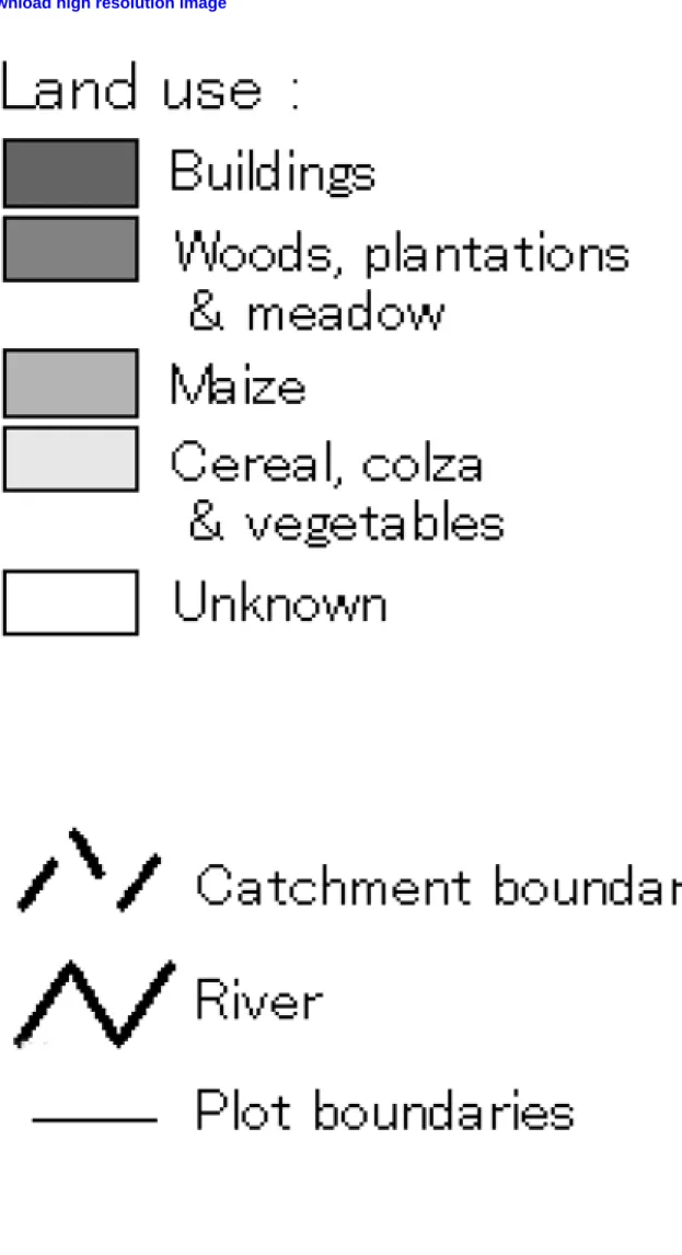
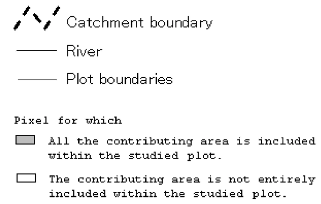
Figure 5. Map of plot contributing areas in the Frémeur catchment. We distinguish areas included
25
within a plot (within-plot contributing areas), from areas partly depending on an upslope plot
26
(upslope-connected plot contributing areas).
1
Figure 6. Cumulative distribution of areas disconnected due to hedgerow network
2
3
Figure 7. Part of the plot outlet tree for the Fremeur catchment
4
5
Figure 8. Part of the arrow diagram showing relations between plots on the Fremeur catchment
6
7
Figure 9. Distribution of the number and the surface area of plot outlet trees versus the number of
8
plots per plot outlet tree, considering all the trees and only the cultivated trees, i.e. including at least
9
one cultivated plot.
10
11
Figure 10. Spatial representation of the plot outlet tree of the Frémeur catchment.
12 13 14 15 16 Tables 17 18
Table 1. Typology of the different objects
19
20
Table 2. Typology of the different plot outlets, pixels and contributing areas
21
22
Table 3. Number of plot outlet versus threshold area used to identify a contributing areaTable 1
23
24 25
Object Type Attribute