Université de Montréal
Gauging the Success of Technical Trading Strategies
in the S&P 500 Index Futures Market
by
Martin Goulet
Department of Economics
Arts & Sciences Faculty
Thesis presented to the Faculté des études supérieures
toward the obtention of the M.Sc. grade
in Economics Sciences
September 2004
Université de Montréal
Faculté des études supérieures
The present thesis entitled:
Gauging the Success of Technical Trading Strategies
in the S&P 500 Index Futures Market
Presented by:
Martin Goulet
was evaluated by the following jury:
René Garcia Ph.D.
Supervisor
Sílvia Gonçalves Ph.D.
ABSTRACT
Technical trading rules are tested to determine their economic and statistical significance as an investment technique using S&P 500 index Futures from 1982 to 2004 and three main subsets of rules: filter rules, trading range breaks and moving average rules. Using a cumulative net profit algorithm designed by Boswijk, Griffioen & Hommes in their 2001 study, we calculate the cumulative net profit of each rule at the end of the initial 12-year period and then compare to a similar test in the 10-year out of sample period. We find that the majority of rules were not consistently profitable within a single period or across both time periods. Individual rules are tested using a makeshift ranking system and it is again found that only a very small fraction of the rules were able to consistently classify as being in the upper rank(s). We then test for the ability to forecast daily Futures returns under the assumption that said returns are identically and independently distributed (IID) and not IID. In either case, only a very small portion of rules demonstrate significant return forecasting ability in the initial or final period. It is concluded that technical trading rules on the whole do not have significant return forecasting power and do not lead to profitable investment decisions which would suggest that technical analysis is not successful in the S&P 500 index Futures market.
TABLE OF CONTENTS
I. INTRODUCTION
1
II. TECHNICAL TRADING IN FUTURES
3
III. REVIEW OF LAST RESEARCH
5
IV. BASIS & METHODOLOGY
12
V. EMPIRICAL ANALYSIS
15
VI. CONCLUSION
23
ALGORITHM & PARAMETERS
26
REFERENCES
30
TABLES & FIGURES LIST
TABLE 1. All Rules Combined Profitability and Significance - Initial Period TABLE 2. All Rules Combined Profitability and Significance - Final Period
TABLE 3. Significance of Difference between Mean Buy and Sell Returns - Initial Period TABLE 4. Summary Statistics of Distribution of Net Profit and Cumulative Returns TABLE 5. All Rules Combined Trading Rule Rankings
TABLE 6. Number of Rules that Performed Equally Well in Both Periods TABLE 7. Specifications of the Nine Best Rules
TABLE 8. Significance of Buy/Sell Dummy Variables when Futures Return Modeled as ARIMA TABLE 9. Significance of Buy/Sell Dummy Variables when Futures Return as GARCH
FIGURE 1. Continuous Series of Futures Prices - Initial Period FIGURE 2. S&P 500 Futures Daily Returns Histogram - Initial Period FIGURE 3. Filter Rule Profitability Histogram - Initial Period
FIGURE 4. Trading Range Break Rule Profitability Histogram - Initial Period FIGURE 5. Moving Average Rule Profitability Histogram - Initial Period FIGURE 6. Filter Rule Profitability Histogram - Final Period
FIGURE 7. Trading Range Break Rule Profitability Histogram - Final Period FIGURE 8. Moving Average Rule Profitability Histogram - Final Period FIGURE 9. All Rules Combined Profitability Histogram - Initial Period FIGURE 10. All Rules Combined Profitability Histogram - Final Period
FIGURE 11. All Rules Combined t ratio (buy/long only) Histogram - Initial Period FIGURE 12. All Rules Combined t ratio (sell/short only) Histogram - Initial Period FIGURE 13. All Rules Combined t ratio (buy/long only) Histogram - Final Period FIGURE 14. All Rules Combined t ratio (sell/short only) Histogram - Final Period
ACKNOWLEDGEMENTS
This research report could not have been completed without the generous help from my professor and research supervisor, René Garcia as well as the contribution of Desjardins Capital in the form of time series data.
I.
INTRODUCTION
Technical analysis is essentially looking at past and present prices of an asset, drawing conclusions about time trends and rendering inferences about future prices. The importance of this question is self-evident, at least where the field of financial economics is concerned. One of the fundamental postulates in financial economic theory is that asset markets are reasonably efficient. The term efficiency is used to denote the property of asset prices to reflect all present and historical public information. Were this not the case, it is argued, investors could make a profit simply by waiting and investing only after the emergence of “good news” (i.e. a firm’s quarterly net earnings have exceeded financial analyst expectations, etc). Several studies have been performed to test the efficiency of asset markets, particularly stock markets in the past fifty years, and it is generally assumed today that financial markets are at least weakly efficient (“weak form efficiency”)1. If financial markets are indeed efficient,
price trend watching techniques should not be profitable since past information should already be factored into the asset’s present price. If technical analysis rules are consistently and significantly profitable then it would indicate that financial markets may not be as efficient as is often thought.
Technical analysis was the forebear of modern finance theory and with the advent of online investing and so-called “day-trading”, it is generally accepted that chartists may indeed have an impact on asset prices and that therefore its study should be undertaken regardless of its credibility as an investment technique. Recent research on heterogeneous agent system models demonstrate that if we include two types of agents in a market: one a fundamental return/risk optimizer and another that looks only at price trends (as do most technical analysts), asset return distributions are characterized by fat tails, autoregressive conditional heteroskedasticity and general return unpredictability2.
The goal of this report is to test whether or not technical trading is truly successful in the index Futures market. The index that shall serve this purpose is the “Standard & Poor’s 500” (S&P 500) index of
1Eugene F. Fama, "Random Walks in Stock Market Prices," Financial Analysts Journal, September/October 1965 (reprinted January-February 1995).
American companies. The stock prices of individual companies within the index are market capitalization weighted and summed with the resulting sum being the spot index price. This particular index is particularly interesting due to its common usage as the proxy for the total market portfolio in other financial models. We define the necessary and sufficient conditions for concluding that technical trading is successful: a large set of trading rules, not just a few, should demonstrate significant return forecasting power and should generate positive trading profits after correcting for transaction costs.
Using a cumulative net profit algorithm designed by Boswijk, Griffioen & Hommes in their 2001 study, we calculate the cumulative net profit of the 4907 rules at the end of the initial 12-year period, accounting for the respective economic costs and benefits of trading in Futures contracts. A 10-year final out of sample period is then used to test the consistency in the profitability of the rules. A profit-based ranking of individual rules will be developed in order to determine the consistency in their performance between periods. Said rankings, although simple and effective, are arbitrary and obviously subject to potential bias and are to be used only as an indication of the quality of particular rules which may or may not already be popular among practitioners.
Firstly, we then test for the rules’ ability to forecast daily Futures returns under the assumption that said returns are identically and independently distributed (IID) by looking at the distribution of their derived profits and the significance of their returns. In the second part of this study, we group the rules that are significant, profitable and that take more than a single position (each rule must advocate more than one position during the period, i.e. a rule can’t advocate a long/short position in the Futures contract for the entire period) in both the initial and final “out of sample” period. We finally test said rules under the assumption of non-IID returns by modeling the time series of Futures returns in the initial period in such a way as to account for serial correlation and volatility clustering. A test of the forecasting ability of each rule is done by measuring the significance of the coefficients of the dummy variable within these regressions (where the dummy variables are the daily position values taken by each rule).
II.
TECHNICAL TRADING IN FUTURES
Technical analysis can be defined as an attempt to predict the performance of a financial asset by spotting trends in price, without regard to the intrinsic nature or situation (economic or fundamental) of the underlying company, instrument, rate or commodity. Those that practice technical analysis are commonly called technical analysts or “chartists” from their predilection for making investment decisions based primarily on graphs or charts of asset prices.
Technical analysis and its respective trading rules come in many forms. In this report, we will confine ourselves to three main types of rules: filter rules, trading range breaks and moving average rules. Filter rules generate buy (sell) signals if the price rises (falls) by x% from a subsequent low (high). Trading range break rules use support and resistance levels defined, in this case, as the local minima and maxima of closing prices. If the price falls (rises) though the local minima (maxima) a sell (buy) signal is generated and a short (long) position is taken in the market. If the price moves between local minima and maxima, the position in the market is maintained until there is a new breakthrough. Moving average rules make use of one or two moving averages of closing prices (in the case only one is used, the price itself is considered the second moving average). A moving average rule using two moving averages of prices uses a fast and a slow moving average. If the fast moving average crosses the slow moving average in an upward (downward) direction, a buy (sell) signal is generated3. When applying technical
analysis on derivatives however, the process becomes more complex.
Futures contracts on indexes are traded on Options & Futures exchanges such as the Chicago Board of Options Exchange Futures Exchange (CBOE Futures Exchange) or the Chicago Mercantile Exchange (CME). The S&P 500 index Futures data used in this report was generously supplied by Desjardins Capitaland is taken from the CME. A concise definition and explanation of a Futures contract is as follows:
“A standardized, transferable, exchange-traded contract that requires delivery of a commodity, bond, currency, or stock index, at a specified price, on a specified future date. Unlike Options, Futures convey an obligation to buy. The risk to the holder is unlimited, and because the payoff pattern is symmetrical, the risk to the seller is unlimited as well. Dollars lost and gained by each party on a Futures contract are equal and opposite. In other words, Futures trading is a zero-sum game. Futures contracts are forward contracts, meaning they represent a pledge to make a certain transaction at a future date. The exchange of assets occurs on the date specified in the contract. Futures are distinguished from generic forward contracts in that they contain standardized terms, trade on a formal exchange, are regulated by overseeing agencies, and are guaranteed by clearinghouses. Finally, by making an offsetting trade, taking delivery of goods, or arranging for an exchange of goods, Futures contracts can be closed.”4
Futures contracts are marked to market every trading day, which entails the elimination of the contract by the clearinghouse at the end of each day and the investor’s margin account be credited (debited) in the case there was a profit (loss) made on the position and then a new identical contract created the following day. In this way, the profits or losses on the position do not accrue to the investor during the entire term to maturity of the contract only to be handed out by the opposing party or clearinghouse on the day of expiration or delivery, as is the case of a Forward contract. In order to transact in Futures contracts, one must “put up” the “initial” margin (similar to a down payment) with the brokerage firm. However, the investor only needs to ensure the margin account balance does not dip below the “maintenance” margin which is usually significantly lower than the initial margin. If this occurs, the investor needs to refill the account back to the initial margin level. On the other hand, if the balance is greater than the initial margin level, the investor may remove (take as net profit) the excess balance. This unique property of Futures contract will be modeled in the algorithm used for this research.
III. REVIEW OF PAST RESEARCH
There have been several attempts to answer the question of the profitability of trading rules in the past. Fama (1965) introduced the idea that returns are unpredictable when conditioned on past returns (i.e. a random walk). In an attempt to measure the profitability of technical trading rules, Fama & Blume (1966) used a filter rule with a 5 to 50% filter on approximately 5 years of data on the thirty individual stocks on the Dow Jones Industrial Average (DJIA) Index and discovered that the filter rule was moderately profitable but only when transaction costs are excluded. The authors consider positive (long) as well as negative (short) positions and compare them to a horizon-length long only strategy. Most of that decade’s research under-estimated technical trading profits and lacked confidence intervals in order to judge the significance of said profits. In order to avoid potential data-mining problems, Fama & Blume calculated average profits per rule or per stock. However, this had the unintended effect of potentially masking the profitability of certain “winning” rules for certain stocks.
Sweeney’s (1986) first analyzed ten exchange rates over a seven year period with seven different rules. After adjusting for transaction costs and risk as defined by the international Capital Asset Pricing Model (CAPM), he finds positive adjusted returns. Critical to his findings was the assumption of normal IID errors when conditioned on the return of the international market portfolio, a rather liberal but common assumption of the simple CAPM, along with the assumption of constant risk premia. Evidently, the problem with using the CAPM as a risk adjuster is the drawbacks of the CAPM itself; the benchmark portfolio must be also be tested as to whether it is a decent proxy of the international total market portfolio. Thus, any test using the CAPM as a risk adjuster is implicitly a joint hypothesis test. Whether this issue has been fully resolved in modern finance theory is still in question. Sweeney (1988) reexamines the research by Fama & Blume and creates a technique used to test the statistical significance of technical trading profits (only filter rules). He assumes that an investor can only take positive positions (no short sales) and reuses individual stocks from the DJIA. However, he only uses stocks that were profitable once filter rules were utilized in Fama & Blume’s original sample period (1957-1962). He then took these “winning” stocks and tested the filter rules using an out of sample time
period (1970-1982) while again assuming constant risk premia and individual asset return variances. Sweeney finds the profitability of the best rules used on the “winning” stocks to be both economically and statistically significant. However, this approach doesn’t seem to be answering the question of whether filter rules of certain specifications render significant profits but rather the question of whether certain stocks are going to be consistent in their returns over several time periods, which in a sense, is completely unrelated to the contribution of the filter rules to these profits.
More recently, Brock, Lakonishok & LeBaron (1992) (BLL hereafter) analyzed the profitability of two types of rules: trading range breaks (“support and resistance” levels) and moving average rules. In their benchmark study, BLL included six permutations of the trading range breaks rule and twenty permutations of the moving average rule. The authors examine the DJIA index itself from 1897 to 1986 and apply the bootstrap technique in order to improve statistical inference. The authors admit to being unable to develop a mathematical test of joint significance for the rules as a group as one would need to understand the complex dependencies between rules in order to do so. The major findings of the research are that the rules are both economically and statistically significant and it is found that the trading rules are able to identify time periods in the index with positive returns on investment and low return volatility and time periods. However, the authors denote the high likelihood of unintended data-mining. Bessembinder & Chan (1998) reexamine the previous study and find that a significant portion of the calculated profits could be largely explained by poor information capture in closing index prices which lead to return measurement errors (“non-synchronous trading”). An important drawback associated with the BLL study and its derivatives is the danger of data-mining, which, although identified by the authors, is not corrected (discussed later).
In order to differentiate their research, Levich & Thomas (1993), examined the profitability of technical trading strategies in a market other than the stock market, namely the foreign exchange Futures market. The authors use a series of prices on a series successive near-term Futures contracts where the US dollar is the reference currency on five foreign currencies and nine trading rules (taken from two main types: filter and moving average rules) from 1976 to 1990. However, they only construct their Futures price series by "pasting" successive contracts at what seems to be only maturity dates rather than rollover
dates. This creates two problems. First, they do not construct an artificial price series by removing the maturity premium on each new contract when “pasting”5 which may generate spurious trends and
returns on “pasting” days that should be earned by the investor and therefore do not represent the true profitability of trading rules. Second, it is unlikely that an investor would or even could physically keep a position in a contract up until the day of maturity, and then still be able to sell it at it’s fundamental price do to a declining lack of liquidity when approaching the maturity date.
A major drawback of the approach taken by previous authors is the ex post identification of optimal trading rules. The issue is subtle yet significant. Due to the possibility of survivor bias, this approach may be testing, in essence, rules that were already deemed to be profitable during the same time period. As financial time series are the most highly scrutinized of time series by practitioners and academics alike, it is inevitable that certain specifications of trading rules (e.g. a filter rule with a 10% filter) would eventually be regarded as being “successful” and therefore worthy of being tested empirically. However, this essentially leads to the testing of whether particular rules are successful at producing significant profits during a time period during which they may have, to a greater degree of probability than would be acceptable compared to one testing a true “universe” of specifications of trading rules, already “survived” by not being “thrown out” by being completely unsuccessful. In essence, there is a greater probability than there should be that rules will render statistically significant profits. Consequently, the survivor bias in the matrix of trading rules also harbors the danger of unintended data-mining: essentially identifying “winning” rules not because they have significant fundamental return forecasting power (which may indicate a causal relationship) but rather simply because they have been successful in past time periods or by other researchers examining the same time series.
In response to this important issue, Sullivan, Timmermann & White (1999) (STW hereafter) completed a comprehensive study of stock and Futures markets. According to the authors, the findings of previous studies, specifically the marked profitability of many trading rules, are largely the result of survivor bias and unintended data-mining. They test this by using a technique (“White’s Reality Check”) that
penalizes possible data-mining effects when bootstrapping data is used. Furthermore, the study was effected using DJIA index price data from 1897 to 1986 (with an out of sample period of 1986 to 1996) and using Futures price data from 1983 to 1986 (with an out of sample period of 1986 to 1996) using six main types of rules with a total of roughly 8000 permutations; a relative “universe” of specifications of rules in order to more easily avoid the data-mining problem. They find the “winning” rules (for the DJIA index) of Brock, Lakonishok & LeBaron (1992) to be still profitable after adjusting for possible data-mining effects, but only for the initial sample time period and not for the out of sample period. The only discernable drawback to the procedure used by STW to examine the profitability of trading in S&P 500 Futures is their very short initial time period which is used to identify the successful trading rules (only three years). Another minor drawback that is shared by the research of Boswijk, Griffioen & Hommes (discussed later) is the usage of a proposed “universe” of rules. Although one can consider nearly 8000 permutations of trading rules to be sufficient in describing all possible specifications, it is still relatively small compared to the theoretically infinite number of specifications that could be used.
Most of the recent academic literature pertaining to technical analysis has focused on the use of genetic algorithms6 (e.g. artificial neural networks) in order to ascertain its potential benefits. The primary
advantage of this approach stems from the machine learning algorithm’s ability to identify “optimal” rules from an almost infinite number of possible specifications, which are derived by ascertaining their ability to generate the best returns on investment (in a previous time period sample), then testing their ability to forecast future returns; an ex ante identification of optimal rules rather than finding the profits (trying to determine the optimal specifications/rules) from a relatively small number of pre-specified rules. As a result, the data-mining problem is less of an issue. A few examples of this type of study are Neely et al. (1997), Gencay (1998, 1999) and Fernandez-Rodriguez et al. (2000). A typical study using the aforementioned genetic programming approach would be that of Allen & Karjalainen (1999). Using daily S&P 500 index prices from 1928 to 1995, it is again found that the trading rules are able to identify time periods in the index with positive returns on investment and low return volatility and time
6Algorithms used to find approximate solutions to difficult-to-solve problems through application of the principles of evolutionary biology to computer science. Genetic algorithms use biologically-derived techniques such as inheritance, mutation, natural selection, and recombination. Genetic algorithms are a particular class of evolutionary algorithms.
periods when the opposite is true. The authors contend that these results can largely be attributed to low order serial correlation in index returns and that, in addition, once adjusted for transaction costs, said rules are no longer profitable in excess of a buy long-term strategy.
The article which served as the basis for this report is the research by Boswijk, Griffioen & Hommes (2001). A simple trading algorithm was designed in order to mimic the actions of 5350 “investors”, each using an individual permutation of one of three types of main trading rules: filter rules, trading range breaks and moving average rules. The algorithm calculates cumulative wealth per rule at the end of the sample period and is designed to replicate the full costs and benefits associated with trading in Futures markets: margin and savings account interest rates, transaction costs and margin calls. They apply this algorithm to Futures on cocoa (with data from the CSCE7 and the LIFFE8) and on the pound
sterling - US dollar exchange rate from 1983 to 1997. The majority of trading rules in the cocoa Futures traded on the LIFFE is found to be profitable whereas trading rules as group perform poorly when applied to the CSCE. Unlike the STW study, their approach tests the real returns of investing in Futures with an algorithm that accounts for margin and savings account and constraints which can become significant when losses from trading rules become substantial and consistent. Although BGH follow the approach used by STW in using a fairly large set of rules (5350), the rules themselves are still pre-specified which leads to the aforementioned inference problems.
The Boswijk, Griffioen & Hommes approach:
¾ A series of artificial Futures returns is constructed by pasting the returns of the series of “second to nearest to delivery” contracts during the period at appropriate rollover dates.
¾ The algorithm gives daily “signals” to take long, short or neutral positions (1,-1, or 0) in the Futures contract. This is done for every trading rule.
7Coffee, Sugar and Cocoa Exchange (in New York) 8London International Financial Futures Exchange
¾ Mean returns and variances for buy/long days and sell/short days are calculated at the end of the period. Cumulative net profits are calculated at the end of the period for every rule.
¾ Tests are done assuming IID returns on the mean returns for buy/long and sell/short days as well as the difference between mean returns for each “type” of day. These tests of average returns are then compared to the profitability (calculated by the cumulative net profit) of each rule.
¾ Second, they dispense with the assumption of IID returns and model the time series of artificial Futures returns using both a GARCH-in-mean and an EGARCH model in order to account for serial correlation in the returns and volatility clustering. They then individually plug buy and sell dummy variables into their models and test for significance of the dummy variable coefficient. This is done for every rule regardless of profitability under cumulative wealth and/or the IID assumption.
¾ Finally, the authors analyze the distribution of the student t ratios of every rule and draw conclusions about the significance of the technical trading rules as a group.
Considering the arguments given previously, the principal difficulty lies in properly discerning the true contribution of trading rules to generated profits. Many of the earlier studies simply created a small number of rules (specifications), tested them on a time series and tabulated the profits derived from each rule. Later studies attempted to test the significance of these profits either by using certain statistical tests that depend on the mathematical construction of these rules or by testing them in out of sample periods (real or bootstrapped). However, due to the presence of potential survivor bias and, consequently, possible unintended data-mining, the results of previous studies were often discounted by researchers in the late 1990’s such as Sullivan, Timmermann & White (1999) who claimed that said results were indeed largely the result of data-mining. The problem stemmed largely from the intense scrutiny of financial time series and the pre-specification of a small number of trading rules. It is inevitable that popular specifications of trading rules (due to success in the past) will be the ones most
tested empirically. There is therefore a disproportionately high probability that these rules will render statistically significant profits. Some attempts have been made to purge possible data-mining effects from the results using statistical techniques (i.e. “White’s Reality Check”9) while others have started
using genetic algorithms that identify optimal trading rules from a practically infinite number of rules, therefore eliminating the danger of survivor bias and reducing the likelihood of data-mining. However, statistical tests such as White’s Reality Check can only be used in certain circumstances and there is no consensus on how genetic algorithms (by what process) should determine truly optimal trading rules. Many of the studies that were reviewed also made understandable but arguable assumptions such as constant risk premia to derive risk-adjusted returns and normality in the errors. Lastly, some suffered from minor oversights such as the direct pasting of Futures price series from one contract to the next, creating possible spurious regression results10. It has generally been the consensus, however, that if
technical trading rules did once produce significant returns in the past, they have ceased to do so since the beginning of the 1990’s.
This study shall follow the approach taken by BGH (2001). Although it suffers from a few minor shortcomings, namely the issue of ex post optimal rule identification from pre-specified rules, it is an objective approach (a large set of rules) that is used in a market that has not been fully explored as of yet (Futures) and accounts for the respective costs and benefits of trading in said market. In this way, it paints a better portrait of the real profitability of trading rules in the Futures market than does any other of the reviewed studies.
9STW (1999)
IV. BASIS & METHODOLOGY
This paper will focus on the profitability of technical trading strategies in the S&P 500 index Futures market rather than the index itself. This has several advantages: dividends are not present and therefore do not lead to a misestimation of daily returns, transaction costs on Futures are much lower than in ordinary equity markets and so a direct comparison the profitability of transaction-heavy rules versus that of less “active” rules and, finally, short positions in Futures markets are always allowed and easily undertaken which, once more, allows a better comparison between rules. This last advantage stems from the fact that, due to the very nature of Futures markets being a zero-sum game (the total number of long and short positions in one contract must be equal to zero); a short position is as easily taken as a long position. In ordinary equities markets, however, an investor would be hard pressed to follow the signals of a rule that are advocating a short position for more than a few consecutive months due to margin calls and the inevitable danger of being forced to repurchase the asset prematurely (“buy in”) if there is a liquidity shortfall (“short squeezed”).
We will answer the question of whether or not technical trading rules are consistently profitable in the S&P 500 Futures market by using the following procedure:
¾ Using the same approach as BGH, an algorithm will calculate the cumulative net profit of 4907 rules that can be classified into three main types: filter rules, trading range breaks and moving average rules. First, we will attempt to improve upon the work by Levich & Thomas (1993) and Brock, Lakonishok and LeBaron (1992) by using a “universe” of trading rules rather than a handful or subset of rules in order to reduce the risk of data-mining. Second, we will improve upon the isolation and identification of “winning” trading rules by using a roughly 12 year “initial” sample time period rather than the three years used by STW. A second improvement on the work of STW (1999) is that it accounts for the respective costs and benefits of trading in Futures contracts (margin calls, borrowing costs, low transaction costs). As a result, it more accurately depicts the profitability of trading rules when applied to the S&P 500 Futures
market. Finally, a 10 year “final” out of sample period will then be used to test the consistency in the profitability of the rules.
¾ We will calculate the percentage of all rules that generate consistent cumulative net profits that have statistically significant forecasting power. This will be accomplished by testing the rules in the first period, identifying the fraction that are profitable, the fraction that are significant (under the hypothesis that daily returns are IID) and those that share both qualities.
¾ Then, we will compare these results to that of the second period. In this way, we are testing the forecasting power of the technical trading rules as a group and not any individual rule.
¾ However, in a slight departure from the BGH model and in an effort to glean more information from the performance of individual rules, rankings and identification based on profitability in one period will be compared to the rankings of profitability in the second period. The fraction of rules that repeated their performance (i.e. managed to achieve the same ranking plus or minus a specified deviation) will be reported. Although essentially ad hoc in nature and therefore not entirely unbiased, the ranking system that was developed is nonetheless very informative if not a completely robust indication of the consistency in the performance of each rule. In order to improve upon the rankings in terms of the quality of the information they present, we need to assume that the “universe” of 4907 rules that were created represent all possible rules11; a closed set of rules in which if a particular rule attains the best ranking in
both periods, one could conclude that it is indeed a well performing rule (the argument that it performed well only because “better” rules were missing from the set would be a non-issue).
¾ Under the assumption that daily returns are non-IID, we attempt to model the time series (first as an ARIMA, then a GARCH model) in order to account for serial correlation and volatility clustering, common traits of financial time series. We test for significance of the forecasting
power of the trading rules by measuring the economic and statistical significance of the coefficients of the daily position dummy variables when inserted into the time series model. However, in a last departure from the BGH approach, instead of testing all rules using this procedure, we test only the “best” rules as defined by their results in the first “IID return” test. This was done due to the extremely involving nature of testing 4907 rules in a regression, another process which would have to be automated (programmed) and which is beyond the scope of this report. Therefore, a working assumption of this particular approach is that once trading rules are considered unsuccessful under the assumption of IID returns, they are not going to be successful under any other time series approximation12.
V.
EMPIRICAL ANALYSIS
The technical trading rule algorithm itself is presented in section “Algorithm and Parameters” on page 26. When taking into account all the parameters of each rule, we end up with 600 different filter rules, 2250 different trading range breaks and 2059 different moving average rules. The algorithm calculates the daily wealth (We) for each rule (as if each rule is an investor who uses only that rule) which is combined from the savings account and the margin account balance at the beginning of each day plus or minus any profit loss derived from the position in the Futures contract. The trading rules generate buy or sell signals at different intervals depending on their specific parameterizations. These signals, in turn, instruct the algorithm to change positions (buy= 1, neutral= 0, short= -1) in the contract by liquidating one contract and/or initializing another and transaction costs (c) are deducted from the margin account. Borrowing in the savings account (i.e. a bank loan) is conducted at a premium (p) over the savings account interest rate (rf_s). Interest is also earned on funds in the margin account (rf_m).
The data used is the series of artificial Futures prices and returns of nearest to expiration, S&P500 Futures from 1982 to 2004. They are the most actively traded and therefore most liquid contracts for this particular underlying asset. This largely ensures against the problems of poor information capture in prices and limits the amount of price “jumps” in the series that might skew algorithm and regression results. As mentioned previously, when using a time series of Futures prices, one cannot simply paste the sequence of relevant Futures contracts together due to the maturity premium attached to the contract with the longest maturity (ceteris paribus). Therefore, as contracts are rolled over, there will often be apparent sudden jumps in the Futures price. These jumps are not the result of supply and demand and therefore do not represent returns earned by the investor or trading rule. Therefore, the returns of each contract must be calculated then pasted back together at the appropriate roll over dates. From these returns, a new “artificial” series of Futures prices is created. If this procedure is disregarded, there will be the aforementioned jumps in price at every rollover date but also the possibility of a spurious upward trend in the time series (see Figure 1).
Transaction costs and margin requirements are widely reported today and are intimately linked with the current price level of the underlying index, we must identify and utilize the costs and margin requirements as percentages of the final period average spot/Futures price and use these relative values (as percentages of the Futures price) when evaluating the initial period. The assumptions used for the inputs in the algorithm are as follows:
¾ We assume that the premium against which can be borrowed per day in the savings account (p) to be roughly 2% per annum (similar to BGH).
¾ We assume that the transaction cost (as a percentage of the Futures price) per trade (c) to be 1.23%. We derive this figure by using the 5$US to 20$US per trade stated on a Futures brokerage website and dividing it by the US$1015 average Futures price (for an average of 1.23%)13.
¾ We assume that the initial margin (im) requirement (as a percentage of the Futures price) to be roughly 8%14. Similarly, we assume that the maintenance margin (mm) requirement (as a
percentage of the Futures price) to be roughly 6.3%15.
¾ We assume that the savings account interest rate daily (rf_s) and the daily margin account interest rate (rf_m) to be equal and that both should be set at the approximate recent 1-year US Certificate of Deposit rate of 2.13% per annum.
¾ In the data given, there was no consistent rollover date used. Rollover dates varied from the 1st to the 10th of the month of expiration. Although inconsistent, this interval is small and therefore acceptable. We assume that 20 days after a rollover date, the position is liquidated and a trade is forced to take place to simulate the effect of contract expirations. This is roughly
13(www.efutures.com)
14We found US$20000 per contract, where one contract = 250 times the price of the index. Therefore, 20000/250 = 80. Thus 80 / {1015 (average Futures price)} = 8% or 0.08.
15We found a price of US$16000 per contract, where one contract = 250 times the price of the index. Therefore, 16000/250 = 64. Thus 64 / {US$1015 (average Futures price)} = 6.3% or 0.063.
the same assumption as used in the BGH study. A twenty day period was used because the last trading day for S&P 500 Futures is the 20th day of the delivery month.
¾ An amount of 100$ was used as the initial investment and credited to the savings account. This was done in order to facilitate the calculation of returns on the Futures series (you need an initial investment in order to calculate returns or else the first return is undefined). Since it is used for every rule, it is arbitrary but irrelevant. As such, a profitable rule is one that produces greater than 100$ of cumulative net profit at the end of the period.
It is not possible to judge directly the significance of the cumulative net profit results. We therefore need to test for significance of the average returns (returns derived from the futures price series) during buy and sell day periods. We do this by finding the total number of buy and sell days (days for which the position is 1 or -1 only) and obtaining the return that was earned on each day. Once the variance of returns on buy and sell days is also obtained, we can then calculate t ratios for the buy day returns and the sell day returns separately. This is done in order to find the individual contribution of each trading rule to buy and sell investment decisions. While there are 3211 observations in the initial time series, only rules with more than 121 buy/sell days (to obtain at least 121 degrees of freedom) were used to ensure that a single critical value could be used for all rules16. Upon closer inspection however, no rule
that generated a t ratio even remotely close to being significant had lower than the required number of days (for either buy or sell respectively). The chosen significance level for all rules was 5% for a critical value of 1.96 with a working hypothesis that the average return should be equal to zero. Rules that generated significant average returns on either buy days, sell days or both were classified as being buy-or-sell significant. Rules that generated significant average returns on buy days as well as sell days were classified as being buy-and-sell significant. Finally the fraction of rules for which a significant difference between the average return during buy days and the average return during sell days was determined. This was done using the working hypothesis that the difference between mean returns should be equal to zero and testing for one-sided significance using the same critical value (but at the
16There were 2308 observations in the final period and the same critical value and significance level was applied. There were also no significant but lower-than-121 buy/sell day rules in the final period.
2.5% level of significance). However, an adjustment for the degrees of freedom known as the Welch Satterthwaite solution for potential heterogeneity of variance was used because the population variances (of returns for buy days and sell days) were not assumed to be similar.
Although used in this section, it should be noted that a very small portion of the rules were not considered for later use in the classification of “best” rules because they simply advocated a buy/long position throughout the entire time period. These were discarded because, first, a long-only position that lasts for the entire period is not trading based on technical analysis in the strict sense of the word and, second, the performance of these rules wouldn’t be particularly informative. Note that all other rules advocated a change of position at least once during the time period (these were named “position varied”).
ECONOMIC SIGNIFICANCE OF THE RULES AS A GROUP
The importance of testing the rules according to cumulative net profit generated during a given period lies in its testing of the economic significance of the profits (which can be translated into returns) after adjusting for all economic and transaction related costs.
In the initial period, 23.1% of all the rules were profitable (see Table 1 and 4 along with Figure 9) and so were 38.8% of filter rules, 23.6% of trading range breaks and 18.0% of moving average rules (see Figures 3, 4 and 5 respectively). In the final (out of sample) period, 36.0% of all the rules were profitable (see Table 2 and 4 along with Figure 10) and so were 31.7% of filter rules, 41.5% of trading range breaks and 31.2% of moving average rules (see Figures 6, 7 and 8 respectively). Therefore, there seems to be have been an increase in the profitability of trading rules between what we could loosely consider the 1980’s and the 1990’s. However, only 12.9% of trading rules were profitable in both periods. In comparison to the findings of the BGH study, these figures are rather low and do not contribute importantly to the rejection of the hypothesis that the use of technical analysis is not economically profitable (when considering the rules as a group or subsets).
RELATIVE ECONOMIC SIGNIFICANCE OF INDIVIDUAL RULES: THE MAKESHIFT RANKING SYSTEM
The rules were first ranked and identified depending on the net profit level derived during the initial period. The rules were then ranked according to their net profit level derived during the final period. Classifications were designed in order to rate the performance of individual rules between periods (see Table 5). Out of 4907 trading rules, we take the “top 500” rules (which translates approximately to the first decile) as an example. A meager 2.6% of rules were able to classify as being in the top 500 during both periods.
In addition, we questioned how many individual trading rules matched the relative initial period performance (and therefore the ranking) in the final period, “give or take” 100 ranking points. An affirmative response was given for only 14.2% of trading rules (see Table 6).
Evidently, these admittedly arbitrary rankings are subject to potential bias and are to be used only as an indication of the quality of particular rules which may or may not already be popular among practitioners. However, it may be indicative of the poor likelihood of obtaining consistent performance from picking any particular rule at random within the group.
STATISTICAL SIGNIFICANCE OF THE RULES AS A GROUP
Under the Assumption of IID Returns
In the initial period, when considering buy-or-sell significance, it was found that 13.7% of the rules classify while 9.3% of all rules are buy-or-sell significant and profitable (under the cumulative net profit test). However, only 7.8% of all rules share the aforementioned properties yet take a position other than a simple long position in Futures contracts for the duration of the period (were position varied). When considering buy-and-sell significance, it was found that none of the rules classify (see Table 1). The distributions, for all rules combined, of the t ratios for buy and then sell significance are displayed in Figures 11 and 12.
In the final period, when considering buy-or-sell significance, it was found that 9.8% of the rules classify while 3.3% of all rules are buy-or-sell significant and profitable (under the cumulative net profit test) whether only position varied or not. When considering buy-and-sell significance, it was found that only 0.1% of the rules classify while none of the rules are buy-and sell significant and profitable, whether position varied or not (see Table 2). The distributions, for all rules combined, of the t ratios for buy and then sell significance is displayed in Figures 13 and 14.
What is most damning of the forecasting power of technical trading strategies is the percentage of rules that generate positive and statistically significant differences between mean buy and mean sell returns. It is demonstrated in Figure 3 that only 1.2% of rules in the initial period and 2.8% of rules in the final period generate a significant difference between mean returns. What this implies is that, under the assumption of IID returns in Futures prices, the buy and sell position “dummy” variables (taken together) of the overwhelming majority of trading rules are not significant in rendering positive returns on investment. In fact, once cumulative profit and variation in position are added to the list of properties, none of the rules remain significant in this regard during the initial period whereas only 0.4% of rules remain so in the final period.
In sum, under the assumption of IID returns, the trading rules as a group generally do very poorly. Although no formal hypothesis testing decision rule was created beforehand, it is submitted that we clearly do not have enough evidence to reject the hypothesis that technical trading rules are of no significant value in the forecasting of returns in the S&P 500 Futures market.
Under the Assumption of non-IID Returns
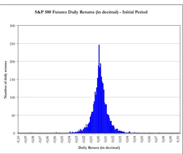
The distribution of artificial daily Futures returns is fairly well centered around its mean and is apparently leptokurtic in comparison to the normal distribution (see Figure 2). It is the general consensus that daily returns on financial assets often exhibit the properties of serial correlation and volatility clustering; properties that violate the assumption of independence between periods and a
constant intertemporal distribution. Therefore, we test for the significance of the coefficients of the buy and sell position “dummy” variables by modeling the artificial time series of daily returns so that it may account for these properties. However, as mentioned previously, we only test the significance of the “best” rules. We define best as those that were profitable according to the cumulative net profit test, buy-or-sell significance (which allows for more rules than the buy-and-sell significance) and position variation (which ensures that actually have a variable that varies at least once). In addition, these rules must have demonstrated these qualities in both time periods. These “best” trading rules and their particular parameterizations are detailed in Table 7.
After ensuring that there are no visible trends or structural changes in the data or unit root (tested by using the augmented Dickey-Fuller tests with various lags), we derive two potential models for the time series: an ARIMA (2, 0, 2) with squared return lags (from t-1 through t-6) as additional explanatory variables and a GARCH (2, 3) model with a simple return lag (t-4). Both models capture the autocorrelation present in the returns. Both models are estimated using the Maximum Likelihood Estimation procedure with and without the Huber-White Sandwich variance/covariance estimator for robust standard errors. An ARCH test of the ARIMA model does not reject the null hypothesis of no autoregressive heteroskedasticity and therefore is suitable for inference. In contrast, a Box-Pierce test of the standardized squared residuals of the GARCH model demonstrates that it fully captures the ARCH effects. Both models were selected to produce residuals that are accepted (non-rejection of the null hypothesis of white noise residuals) as a white noise according to Box-Pierce tests (once again, the GARCH residuals require standardization, i.e. dividing each residual by its standard deviation) and to maximize the absolute value of the Akaike Information Criteria (AIC) or the Schwartz-Bayesian Information Criteria (BIC).
By altering the time series of position variables (which can be equal to 1, 0 or -1) we obtain a set of true dummy variables that take only the appropriate values (only 0’s and 1’s) and then insert them into each model. At this point, we need only take the t ratios from the respective coefficients to determine their significance (a two-sided test). Since we have 9 “best” rules with a string of buy and sell dummy variables each, we have 18 regressions to carry out.
As can be seen in Table 8, under the ARIMA model, only one of the 9 dummy coefficients (composed of rule 1 and rule 8) is significant at the 5% level (when not using robust estimation). When either decreasing the level of significance to 1% or using robust estimation, none of the dummy coefficients are significant. As can be seen in Table 9, under the GARCH model, the rules fair slightly with two dummy coefficients (the buy and sell dummies of rule 2) being significant at the 10% level under robust estimation and the same two coefficients being significant at the 1% level under regular estimation.
We defined the return forecasting power of the best nine trading rules as the contribution of the buy/sell position dummies to daily Futures returns. We measured this contribution by determining the significance of the coefficients of said variables in two separate regressions with the daily returns as the dependent variable. It is determined that only a fraction of these nine rules demonstrated significant return forecasting power. Therefore, under the assumptions outlined previously, it is submitted that the technical trading rules as a group do not have significant return forecasting power and do not lead to profitable investment decisions. This finding, under the assumption of non-IID daily returns, reinforces the earlier conclusion we had reached under the assumption of IID daily returns.
This study only documents the economic and statistical performance of technical trading rules when applied to a single market. However, the same framework can be applied to any market. In order to asses the profitability of technical analysis and its many derivative trading rules, it is necessary to test a large class of rules, as was done in this study. We conclude that a necessary condition for concluding that technical trading is successful is that a large set of trading rules, not just a few, should demonstrate significant forecasting power. If only a few trading rules do so, this may simply be due to chance or to data mining. However, this condition is not sufficient in it of itself to determine that technical trading rules are successful. It is also necessary to that these rules generate positive trading profits after correcting for transaction costs.
VI. CONCLUSION
Technical analysis is essentially looking at past and present prices of an asset, drawing conclusions about time trends and rendering inferences about future prices. Therefore, if financial markets are efficient, such methods should not be profitable since past information should already be factored into the asset’s present price. Therein lies the importance of the question of whether or not technical trading rules can be applied successfully in the Futures market.
We test the profitability of technical analysis using S&P 500 index Futures from 1982 to 2004. We confine ourselves to three main types of rules: filter rules, trading range breaks and moving average rules with different specifications of each rule (600, 2250 and 2057 respectively). Furthermore, we define the necessary and sufficient conditions for concluding that technical trading is successful: a large set of trading rules, not just a few, should demonstrate significant return forecasting power and should generate positive trading profits after correcting for transaction costs.
There have been several attempts to answer the question of the success of trading rules by other researchers. The difficulty, however, lies in properly discerning the true contribution of trading rules to generated profits and accounting for the potential danger of data mining. Using a cumulative net profit algorithm designed by Boswijk, Griffioen & Hommes in their 2001 study, we calculate the cumulative net profit of the 4907 rules at the end of the initial 12-year period, accounting for the respective economic costs and benefits of trading in Futures contracts. A 10-year final out of sample period is then used to test the consistency in the profitability of the rules. In the first period, 23.1% of all the rules were profitable and this figure climbed to 36.0% in the final period. However, we test for consistent profitability and find that only 12.9% of rules qualified as profitable in both periods. Moreover, only 2.6% of the rules were able to classify as being in the top 500 during both periods when ranked according to generated net profit and only 14.2% of rules were able to match the relative initial period performance in the final period (plus or minus 100 ranking points).
We then test for the ability to forecast daily Futures returns under the assumption that said returns are identically and independently distributed (IID). We find that only 1.2% of rules in the initial period and 2.8% of rules in the final period generate a significant difference between mean returns. Thus, the overwhelming majority of trading rules do not have significant return forecasting power. When cumulative profit and variation in position (which entails that no rules can have a single position during the entire length of the period) are considered in addition to forecasting power, none of the rules remain significant in this regard during the initial period whereas only 0.4% of rules remain so in the final period. As a result, the trading rules as a group are deficient in predicting daily Futures returns.
We now test a fraction of the rules, those considered to be the best rules based on economic profitability and IID return forecasting significance, under the assumption that returns are not IID. We define the return forecasting power of the best nine trading rules as the contribution of the buy/sell position dummies to daily Futures returns. We measure this contribution by determining the significance of the coefficients of said variables in two separate regressions with the daily returns as the dependent variable. Only a small fraction (2 out of 9 for the first regression and 1 out of 9 for the second) of these nine rules demonstrates significant return forecasting power.
In conclusion, it is therefore submitted that technical trading rules on the whole do not have significant return forecasting power and do not lead to profitable investment decisions. This would suggest that technical analysis is not successful in the S&P 500 index Futures market. This finding is identical whether or not we assume daily Futures returns to be IID or not.
We conclude that in order to asses the profitability of technical analysis, it is necessary to test a large class of rules for economic profitability after all costs have been subtracted as well as significance in return forecasting power. In our study, we applied each specification of the trading rules consistently during both time periods. It should be noted that, in practice however, technical analysts do not apply one rule (or specification of rules) consistently during a given period when trading in financial securities. They use a combination of rules that changes depending on price trends and perhaps even fundamental values underlying the security in question, sometimes using rules simply because they
generated the greatest returns when fitted to some past period of data. Academics would decry this inconsistency as merely a lack of objectivity and a result of serious data-mining at its worst. However, if we are truly to test the contribution that can be made by technical analysis to the field of financial investment, we must develop tools that allow us to mimic the way such analysts ply their trade. In this regard, further research must accommodate these techniques and test their results accordingly. Genetic programs and their kin are perfect examples of such tools.
ALGORITHM & PARAMETERS
EXPLANATION OF VARIABLES AND ASSSUMPTIONS
p: Borrowing lending over lending premium daily rate of interest: p=0.00004795
c: Transaction costs as a percentage of the Futures price: c=0.001
im: Initial margin as a percentage of the Futures price: im=0.075
mm: Maintenance margin as a percentage of the Futures price: mm=0.05
rf_s: Daily risk-free rate of interest on savings account: rf_s=0.000056164
rf_m: Daily risk-free rate of interest on the margin account: rf_m=0.000056164
Mb: Margin at the beginning of day i
Me: Margin at end of day i
Sb: Savings account balance at beginning of day i
Se: Savings account balance at end of day i
Wb: = Sb + Mb, Total Wealth at beginning of day i
We: = Se + Me, Total Wealth at end of day i
Pos: Position in the Futures (long/buy=1, neutral=0, short/sell=-1) on day i
Pos_old: Position in the Futures on day i-1
P[I]: Price of the Futures Contract on day i
P[I-1]: Price of the Futures Contract on day i-1
PARAMETERS OF TECHNICAL TRADING RULES
Delay: number of days a trading signal must hold before a trade takes place Fixed Holding Period: number of days a position is held, ignoring all other signals n: length of the period (in days) to find local minima (support) and maxima (resistance) Band: percentage band filter
K: fast moving average number of days over which the price must be averaged Percentage: percentage filter (percentage of Futures Price)
PARAMETER VALUES:
Delay parameters = {0,2,3,4,5}
Fixed Holding Period parameters = {0,5,10,25,50} n parameters = {5,10,15,20,25,50,100,150,200,250}
Band parameters = {0,0.001,0.005,0.01,0.015,0.02,0.03,0.04,0.05} N parameters = {1,2,5,10,15,20,25,30,40,50,75,100,125,150,200,250} K parameters = {1,2,5,10,15,20,25,30,40,50,75,100,125,150,200,250}
Percentage (percent) parameters = {0.005,0.01,0.015,0.02,0.025,0.03,0.035,0.04,0.045,0.05,0.06,0.07, 0.08,0.09,0.1,0.12,0.14,0.16,0.18,0.2,0.25,0.3,0.4,0.5}
DAILY WEALTH ALGORITHM 17
Margin account values: If there is NO trade
AND mm*P[I-1] < Me_old (balance has not dipped below the maintenance margin) AND Me_old <= im*P[I-1] (balance is still below initial margin)
Then, Mb=(Me_old)*|Pos| Or else, Mb=im*P[I-1]*|Pos|
Me=Mb*(1+rf_m) + (P[I] - P[I-1])*Pos_old
Costs:
Costs per trade or rollover of contracts: Costs=c*P[I-1]*abs(Pos_old) + c*P[I-1]*|Pos| When no trades take place: Costs=0
Savings account values:
Sb=Se_old + (Me_old - Mb) - Costs
If Sb>0 (you have not borrowed in the savings account to fill up the margin account) Then, Se= Sb*(1+rf_s)
Or else, Se=Sb*(1+rf_s+p)
Cumulative wealth at day i: Wb[I]=Mb + Sb
We[I]=Me + Se
BASIC FILTER RULE
Determining the Position in the market (for every day i):
Repeat for all j=1 to 20 by increments of 1 (twenty days to find the local minima/maxima was used) If (i<j) stop this procedure and do not calculate the next steps
If (P[i-j]>P_max) then, P_max=P[i-j] If (P[i-j]<P_min) then, P_min=P[i-j]
If (P[i] <= P_max*(1 - percent)) (where percent is a parameter to be chosen) Then, Pos=-1;
Or else if (P[i] >= P_min*(1 + percent)) Then Pos=1;
Or else, Pos=Pos_old;
BASIC TRADING RANGE BREAK
Determining the Position in the market (for every day i): If (i>n)
(by increments of 1)
If (P[i-j]>P_max) P_max=P[i-j], Or else nothing changes If (P[i-j]<P_min) P_min=P[i-j], Or else nothing changes
Or else, P_max=99999 (some arbitrary high number that the Futures price will never reach) P_min=0 (number that the Futures price will never reach by construction)
If P[i]>(1 + band)*P_max, then Pos=1 (where band is a chosen parameter) Or else if P[i]<(1-band)*P_min, then Pos=-1
Or else Pos=Pos_old;
BASIC MOVING AVERAGE RULE
Determining the Position in the market (for every day i):
Ma_n_tot=0 (this are to make sure that these variables are reset to 0 at the beginning of every day) Ma_k_tot=0
If i>N (calculate as long as there is enough time passed to have a moving average of N days) For all j =0 to j<K by increments of one, (to sum the K prices)
Ma_k=P[i-j]
Ma_k_tot=Ma_k_tot + Ma_k
For all j=0 to j<n by increments of one, (to sum the N prices) Ma_n=P[i-j];
Ma_n_tot=Ma_n_tot + Ma_n;
Then, Ma_k=Ma_k_tot/k (calculation of the fast moving average)
Then, Ma_n=Ma_n_tot/n (calculation of the slow moving average) Or else, Ma_k=0
Ma_n=0
If K = 1, then Ma_k=P[i], Or else nothing changes If Ma_k>(1 + band)*Ma_n, then Pos=1;
Or else if (Ma_k<(1 - band)*Ma_n), Pos=-1 Or else, Pos=Pos_old;
REFERENCES
1. Allen, F. and R. Karjalainen. (1999). “Using Genetic Algorithms to Find Technical Trading Rules.” Journal of Financial Economics 51, 245-271.
2. Bessembinder, H. and K. Chan. (1998). “Market Efficiency and the Returns to Technical Analysis.” Financial Management 27, 5-17.
3. Boswijk, P., G. Griffioen, and C. Hommes. (2001). “Success and Failure of Technical Trading Strategies in the Cocoa Futures Market.” Tinbergen Institute Discussion Papers, 2001, Tinbergen Institute.
4. Brock, W., J. Lakonishok, and B. LeBaron. (1992). “Simple Technical Trading Rules and the Stochastic Properties of Stock Returns.” Journal of Finance, 47, 1731-1764.
5. Brock, W. and C. Hommes. (1999). “Rational Animal Spirits.” The Theory of Markets, 1999, 109-137.
6. Fama, E. F. and M. E. Blume. (1966). “Filter Rules and Stock-Market Trading.” Journal of Business 39, 226-241.
7. Fernandez-Rodriguez, F., C. Gonzalez-Martel, and S. Sosvilla-Rivero. (2000). “On the Profitability of Technical Trading Rules Based on Artificial Neural Networks: Evidence from the Madrid Stock Market.” Economics Letters 69, 89-94.
8. Gencay, R. (1998). “The Predictability of Security Returns with Simple Technical Trading Rules.” Journal of Empirical Finance 5, 347-359.
9. Gencay, R. (1999). “Linear, Non-Linear and Essential Foreign Exchange Rate Prediction with Simple Technical Trading Rules.” Journal of International Economics 47, 91-107.
10. Levich, R. M. and L. R. Thomas. (1993). “The Significance of Technical Trading-Rule Profits in the Foreign Exchange Market: A Bootstrap Approach.” Journal of International Money and Finance 12, 451-474.
11. Neely, C. J., P. Weller, and R. Dittmar. (1997). “Is Technical Analysis in the Foreign Exchange Market Profitable? A Genetic Programming Approach.” Journal of Financial and Quantitative Analysis 32, 405-426.
12. Sullivan, R., A. Timmermann, and H. White. (1999). “Data-Snooping, Technical Trading Rule Performance, and the Bootstrap.” Journal of Finance 54, 1647-1691.
13. Sweeney, R. J. (1986). “Beating the Foreign Exchange Market.” Journal of Finance 41, 163-182.
14. Sweeney, R. J. (1988). “Some New Filter Rule Tests: Methods and Results.” Journal of Financial and Quantitative Analysis 23, 285-300.
TABLES & FIGURES
TABLE 1. All Rules Combined Profitability and Significance - Initial Period (1982-1994)
Any Buy AND Sell Significant Buy OR Sell Significant
Any 100,0% (4907) 0,0% 13,7%
Profitable 23,1% 0,0% 9,3%
Profitable and Position Varied 18,6% 0,0% 7,8%
All Rules Combined Profitability and Significance - Initial Period (1982-1994)
(percent of all 4907 rules)
TABLE 2. All Rules Combined Profitability and Significance - Final Period (1995-2004)
Any Buy AND Sell Significant Buy OR Sell Significant
Any 100,0% (4907) 0,1% 9,8%
Profitable 36,0% 0,0% 3,3%
Profitable and Position Varied 22,8% 0,0% 3,3%
All Rules Combined Profitability and Significance - Final Period (1995-2004)
TABLE 3. Significance of Difference between Mean Buy and Sell Returns - Initial Period (1982-1994)
Any Profitable
Profitable and Position Varied
1,2% 2,8%
INITIAL PERIOD FINAL PERIOD
All Rules Combined Significance of Difference Between Means
(percent of all 4907 rules)
Significant Difference Between Mean Returns
0,0%
0,0% 0,4%
0,4%
TABLE 4. Summary Statistics of Distribution of Net Profit and Cumulative Returns
Net Profit (US$) Return (%) Net Profit (US$) Return (%)
average net profit: -221,27 -3,21 -590,19 -6,90
std. deviation: 563,64 5,64 1289,09 12,89
skewness coefficient: -4,17 -4,17 -3,95 -3,95
kurtosis coefficient: 39,77 39,77 37,51 37,51
Summary Statistics
TABLE 5. All Rules Combined Trading Rule Rankings
FINAL PERIOD BOTH PERIODS
Profitable 36,0% 12,9% Top 10 0,2% 0,0% Top 50 1,0% 0,0% Top 100 2,0% 0,0% Top 200 4,1% 0,1% Top 500 10,2% 2,6% Top 1000 20,4% 20,4% 8,0% INITIAL PERIOD
Rankings Within and Between Periods
(percent of all 4907 rules)
23,1% 0,2% 1,0% 2,0% 4,1% 10,2%
TABLE 6. Number of Rules that Performed Equally Well in Both Periods
Attained Initial Position
+/- 100 Ranking Points 14,2%
Relative Performance of Each Rule - Final Period (1995-2004)
(percent of all 4907 rules)
TABLE 7. Specifications of the Nine Best Rules
Variable # Rule ID Rule Type K N Band/ Delay Fixed Holding
Percentage Period
dummy 1 rule 3097 moving average 1 200 0,04 0 0
dummy 2 rule 3898 moving average 5 10 0,04 0 0
dummy 3 rule 3111 moving average 1 200 0,05 0 0
dummy 4 rule 3215 moving average 1 150 0,04 0 0
dummy 5 rule 776 trading range break 0 5 0,04 0 0
dummy 6 rule 3522 moving average 10 75 0,05 0 0
dummy 7 rule 2970 moving average 1 250 0,04 0 0
dummy 8 rule 977 trading range break 0 10 0,03 0 5
dummy 9 rule 1001 trading range break 0 10 0,04 0 0