Titre: Title:
A hybrid numerical-semi-analytical method for computer
simulations of groundwater flow and heat transfer in geothermal borehole fields
Auteurs:
Authors: Massimo Cimmino et Bantwal Rabi Baliga Date: 2019
Type: Article de revue / Journal article Référence:
Citation:
Cimmino, M. & Baliga, B. R. (2019). A hybrid numerical-semi-analytical method for computer simulations of groundwater flow and heat transfer in geothermal borehole fields. International Journal of Thermal Sciences, 142, p. 366-378. doi:10.1016/j.ijthermalsci.2019.04.012
Document en libre accès dans PolyPublie Open Access document in PolyPublie
URL de PolyPublie:
PolyPublie URL: https://publications.polymtl.ca/5502/
Version: Version finale avant publication / Accepted versionRévisé par les pairs / Refereed Conditions d’utilisation:
Terms of Use: CC BY-NC-ND
Document publié chez l’éditeur officiel
Document issued by the official publisher
Titre de la revue:
Journal Title: International Journal of Thermal Sciences (vol. 142)
Maison d’édition:
Publisher: Elsevier
URL officiel:
Official URL: https://doi.org/10.1016/j.ijthermalsci.2019.04.012
Mention légale:
Legal notice: ©2019. This manuscript version is made available under the CC-BY-NC-ND 4.0 licensehttp://creativecommons.org/licenses/by-nc-nd/4.0/
Ce fichier a été téléchargé à partir de PolyPublie, le dépôt institutionnel de Polytechnique Montréal
This file has been downloaded from PolyPublie, the institutional repository of Polytechnique Montréal
1
A hybrid numerical-semi-analytical method for computer simulations of
groundwater flow and heat transfer in geothermal borehole fields
Massimo Cimmino
a§, Bantwal R. (Rabi) Baliga
baÉcole Polytechnique de Montréal, Département de génie mécanique
Case Postale 6079, succursale “centre-ville”, Montréal, Québec, Canada H3C 3A7 §Corresponding author: [email protected]
bDepartment of Mechanical Engineering, McGill University 817 Sherbrooke St. W., Montreal, Quebec H3A 0C3, Canada
2
A hybrid numerical-semi-analytical method for computer simulations of
groundwater flow and heat transfer in geothermal borehole fields
Abstract
The formulation of a hybrid numerical-semi-analytical method for cost-effective simulations of heat transfer in fields of vertical geothermal boreholes, in the presence of groundwater flow, is presented. An amalgamation of a co-located control-volume finite element method and a finite volume method is used to solve 1) a volume-averaged continuity and the Darcy-Brinkman-Frochheimer equations to obtain the distribution of the groundwater flow; and 2) an unsteady three-dimensional volume-averaged advection-conduction equation to calculate the related ground temperature distribution, assuming local thermodynamic equilibrium between the groundwater and the soil particles. The bulk temperature distribution of the working fluid (flowing inside the legs of a U-tube pipe inserted inside each borehole and kept in place by grout) and the related heat extraction (or addition) rate are obtained using a semi-analytical method to solve a quasi-steady quasi-one-dimensional model. The conditions of no-slip, impermeability, equality of temperature, and continuity of heat flux are used at the interface between each borehole and the groundwater-saturated soil in the borehole field. The proposed method is applied to test and demonstration problems to demonstrate its capabilities.
Key words: Geothermal borehole fields; groundwater flow; hybrid numerical-semi-analytical
method; Darcy-Brinkman-Forchheimer equations; volume-averaged advection-conduction equation; control-volume finite element method
3
1. Introduction
Geothermal systems are playing an increasingly important role in ongoing worldwide efforts to develop environmentally friendly, sustainable, and efficient ways of fulfilling space heating and cooling demands. A promising approach in this regard is based on ground-source heat pumps (GSHPs) coupled to vertical geothermal boreholes (hereafter referred to as boreholes in this paper) [Spitler (2005); Kavanaugh and Rafferty (2014)]. Designing of GSHPs is facilitated by accurate predictions of the working-fluid and ground temperatures, and the related heat extraction and injection rates, during their operation. The techniques used for such predictions are often based on mathematical models that invoke the assumption of purely conductive heat transfer in the ground that surrounds the boreholes [Yang et al. (2010); Li and Lai (2015)]. However, if the flow of groundwater in a borehole field is sufficiently high, it could have a significant effect on the temperatures of the ground and the boreholes, and the related heat transfer rates, as discussed by Chiasson et al. (2000), Fan et al. (2007), Wang et al. (2009), Chiasson and O’Connell (2011), Zanchini et al. (2012), Capozza et al. (2013), Hecht-Méndez et al. (2013), and Choi et al. (2013), for example.
Accounting for the effects of groundwater flow has also resulted in several improvements to the analyses of geothermal thermal-response tests and the data deduced from them, as demonstrated, for example, by the works of Gehlin and Hellström (2003), Lee and Lam (2012), Therrien et al. (2010), Raymond et al. (2011), Wagner et al. (2013), Rouleau and Gosselin (2016), Rouleau et al. (2016), and Zhang et al. (2016). It should also be noted that the heterogeneity of the soil hydraulic conductivity and the mixing of flowing groundwater at the pore scale, could create disparities between the longitudinal (parallel to the direction of groundwater flow) and the transverse (perpendicular to the direction of groundwater flow)
4 dispersion of heat, as discussed, for example, in the works of Hsu and Cheng (1990), Metzger et al. (2004), Hidalgo et al. (2009), Hecht-Méndez et al. (2010), Diersch et al. (2011a; 2011b), Molina-Giraldo et al. (2011a), Chiasson and O’Connell (2011), and Nield and Bejan (2013). Furthermore, in soils of sufficiently high hydraulic conductivity, buoyancy-driven natural convection can also affect the performance of geothermal systems, as shown, for example, in the works of Zhao et al. (2008) and Ghoreishi-Madiseh et al. (2013).
Analytical solutions to several simplified mathematical models of heat transfer in borehole fields with uniform groundwater flow have been proposed. They are based on adaptations and extensions of the seminal works of Carslaw and Jaeger (1959), Eskilson (1987), and Hellström (1991). These analytical approaches typically employ moving-infinite-line-source and moving-finite-line-source techniques, as illustrated, for example, in the works of Sutton et al. (2003), Diao et al. (2004), Molina-Giraldo et al. (2011b), Tye-Gingras and Gosselin (2014), and Rivera et al. (2015). Erol et al. (2015) have used a moving-finite-line-source model for investigating heat transfer in borehole fields with groundwater flow and different longitudinal and transverse thermal conductivities (to account for the effects of thermal dispersion).
Compared to analytical methods, such as those mentioned above, numerical methods offer enhanced accuracy in the simulation of heat transfer in borehole fields [Yang et al. (2010)]. Numerical simulations of unsteady heat transfer in borehole fields, without and with groundwater flow, and based on finite difference, spectral, unstructured finite volume, and finite element methods, are discussed, for example, in the works of Rottmayer et al. (1997), Yavuzturk et al. (1999), Li and Zheng (2009), Bauer et al. (2011), Al-Khoury and Focaccia (2016), and Dai et al. (2016). However, unsteady and fully multidimensional numerical simulations of the heat transfer processes in borehole fields, in both the ground and the boreholes, are quite expensive
5 computationally [Yang et al. (2010)]. Thus, for incorporation in design and energy-analysis procedures for borehole fields, hybrid numerical-analytical and numerical-semi-analytical methods, in which numerical simulations of heat transfer in the ground are coupled with approximate analytical or semi-analytical solutions of heat transfer in the boreholes (including the working fluid flowing through the U-tubes inserted in them), are an attractive cost-effective alternative (offering acceptable accuracy at affordable costs) to fully numerical and also completely analytical methods [Yang et al. (2010); Li and Zheng (2009); Bauer et al. (2011); Choi et al. (2013)].
In this paper, the formulation of a hybrid numerical-semi-analytical method for cost-effective simulations of heat transfer in borehole fields in the presence of groundwater flow is presented; it is then checked against a moving-finite-line-source analytical solution for a simplified version of the problem of interest; and, finally, its application to a demonstration problem and the results are discussed. In this method, an amalgamation of a co-located control-volume finite element method and a finite control-volume method (CVFEM and FVM) [Baliga and Atabaki (2006); Lamoureux and Baliga (2011)] is used to solve 1) a volume-averaged continuity equation and the Darcy-Brinkman-Frochheimer equations to obtain the distribution of the groundwater flow (assumed to be steady and two-dimensional in the horizontal cross-section of the borehole field); and 2) an unsteady three-dimensional volume-averaged advection-conduction equation to calculate the ground temperature distribution, assuming local thermodynamic equilibrium between the groundwater and the soil particles [Vafai (2005); Nield and Bejan (2013)]. The bulk temperature distribution of the working fluid (flowing inside the legs of a U-tube pipe inserted inside each borehole and kept in place by grout) and the heat extraction (or addition) rates are obtained using a semi-analytical solution to a quasi-steady
6 quasi-one-dimensional model, based on the concept of a delta-circuit of thermal resistances [Hellström (1991)].
The hybrid numerical-semi-analytical method proposed in this paper follows the works of Bernier and Baliga (1992) and Lamoureux and Baliga (2015), who proposed cost-effective hybrid methods for computer simulations of closed-loop thermosyphons, and Cotta and Mikhailov (2006). It also complements and extends the following two hybrid methods proposed for the investigation of heat transfer in borehole fields: 1) the method of Li and Zheng (2009), who used an unstructured cell-centered finite volume method for simulations of unsteady three-dimensional pure conduction heat transfer in the ground and a quasi-steady quasi-three-dimensional model [Yang et al. (2010)] for calculating the bulk temperature distribution of the working fluid; and 2) the method of Choi et al. (2013), who used a commercial finite element code (COMSOL Multiphysics 4.2a) to solve a two-dimensional steady version of the Darcy equation [Vafai (2005); Nield and Bejan (2013)] for the groundwater flow and a transient volume-averaged two-dimensional convection-conduction equation for heat transfer in the ground, and coupled these numerical solutions with an analytical solution of a model of the average (arithmetic mean) of the inlet and outlet bulk temperatures of the working fluid flowing through the U-tubes inserted in the boreholes.
2. Layout of the borehole field and related notation
Attention in this work is focused on vertical boreholes, each with a single U-tube pipe inserted symmetrically within it and held in place by grout. The vertical and horizontal cross sections of a borehole, 𝑛, are shown in Fig. 1. There are 𝑁𝑏 such boreholes in the field of interest. Each of these boreholes has an active (or heated) length 𝐻 and a radius 𝑟𝑏; and the active length starts at
7 a depth 𝐷 below the ground surface. The working (or heat carrier) fluid flows through each borehole at a mass flow rate of 𝑚̇𝑓 through a U-tube pipe of inner radius 𝑟𝑝,𝑖 and outer radius 𝑟𝑝,𝑜. The ground surface or top boundary of the borehole field is indicated by Γ𝑇, the interface between borehole 𝑛 and the surrounding ground in the borehole field is denoted by Γ𝑏,𝑛, and the vertical coordinate 𝑧 starts at the ground surface and is directed downwards. The boreholes are evenly spaced on a square grid, with a distance 𝐵 between adjacent boreholes, as indicated in Fig. 2 for a field of 3 × 2 boreholes. The east, west, north, and south boundaries of the borehole field (see Fig. 2) are denoted by Γ𝐸, Γ𝑊, Γ𝑁, and Γ𝑆, respectively; and the groundwater enters the borehole field with a uniform velocity, 𝑈∞, and temperature, 𝑇𝑔, across the full west boundary, Γ𝑊.
Figure 1. Schematic representations of the vertical (left) and horizontal (right) cross-sections of
8
Figure 2. Schematic representation of a horizontal cross-section of the borehole field and the
related notation
3. Mathematical models of groundwater flow, temperature distributions, and heat transfer in the borehole field
The assumptions invoked in these mathematical models are presented first in this section. Then the equations that were used to model the groundwater flow in the borehole field, the related temperature distribution and heat transfer in the groundwater-saturated soil, and the temperature distribution and heat transfer in each borehole, in that order, are presented.
3.1. Assumptions
The following assumptions are invoked in the mathematical models adopted in this work:
• The thermophysical properties of the dry soil in the borehole field, and also the grout and U-tube pipe wall in the boreholes, are uniform and constant
• The groundwater is an incompressible Newtonian fluid and its thermophysical properties are uniform and constant
9 • The soil in the borehole field is fully saturated with groundwater, and it has uniform and
constant effective thermophysical properties
• On the entire west boundary (span and depth) of the borehole field, the groundwater velocity (magnitude and direction) and temperature (denoted by 𝑈∞ and 𝑇𝑔, respectively, as shown in Fig. 2) are spatially uniform and invariant in time
• The groundwater-saturated soil in the borehole field is initially at a spatially uniform temperature 𝑇𝑔 (or the initial geothermal gradient in the domain of interest is considered insignificant)
• The ground-surface (𝑧 = 0) temperature remains constant throughout and is equal to the initial undisturbed ground temperature 𝑇𝑔
• Buoyancy-driven natural convection is negligibly small, both in the groundwater and in the working fluid (flowing through the U-tube pipe in each of the boreholes)
• The groundwater flow is effectively steady and two-dimensional in the horizontal cross-section of the borehole field
• There is local thermodynamic equilibrium between the groundwater and the soil particles, thus the local intrinsic phase-average temperatures of the soil particles and the groundwater are effectively the same and governed by a single volume-average advection-conduction equation [Vafai (2005); Nield and Bejan (2013)]
• The viscous dissipation and the thermal dispersion due to groundwater movement are negligible
• The effects of the thermal capacitance of each borehole (grout, U-tube pipe wall, and the working fluid flowing in it) are negligible, so the heat transfer inside the boreholes is effectively quasi-steady
10 • In the working fluid flowing in the U-tube pipe in each of the boreholes, conduction in the axial (or mean flow) direction (z) is negligible compared to advection, viscous dissipation is negligible, the thermophysical properties are constant (equal to values at the arithmetic-mean of the inlet and outlet bulk temperatures), and hydrodynamically and thermally fully developed turbulent flow prevails [Incropera and DeWitt (2002)]
The assumptions of effectively steady and two-dimensional groundwater flow in the horizontal cross-section of the borehole field, and negligible effects of buoyancy, can be avoided by using a numerical solution of the unsteady, three-dimensional, versions of the volume-averaged continuity and Darcy-Brinkman-Forchheimer equations (including buoyancy terms) [Vafai (2005); Nield and Bejan (2013)]. Furthermore, the assumption of quasi-steady heat transfer in the boreholes can be avoided by using a thermal-resistance-capacitance model (TRCM), similar to the one proposed by Bauer et al. (2011), and getting guidance from the works of Pasquier and Marcotte (2012) and Beier (2014). However, the above-mentioned assumptions were invoked in this work to keep the demonstration of the proposed hybrid method relatively simple and cost-effective, and the aforementioned ways to avoid these assumptions are considered as potential extensions of the work presented in this paper.
3.2. Groundwater flow
The following volume-averaged continuity and Darcy-Brinkman-Forchheimer equations [Vafai and Tien (1981); Vafai (2005); Nield and Bejan (2013)] were used to model the steady two-dimensional groundwater flow in the horizontal cross-section of the borehole field:
𝜕 𝜕𝑥𝑢𝑥+
𝜕
11 𝜌𝑤 𝜀2 (𝑢𝑥 𝜕 𝜕𝑥𝑢𝑥+ 𝑢𝑦 𝜕 𝜕𝑦𝑢𝑥) = − 𝜕 𝜕𝑥𝑃 + 𝜇𝑤 𝜀 ( 𝜕2 𝜕𝑥2𝑢𝑥+ 𝜕2 𝜕𝑦2𝑢𝑥) − 𝜇𝑤 𝐾 𝑢𝑥− 𝜌𝑤𝐶𝐹 √𝐾 𝑢𝑢𝑥 𝜌𝑤 𝜀2 (𝑢𝑥 𝜕 𝜕𝑥𝑢𝑦+ 𝑢𝑦 𝜕 𝜕𝑦𝑢𝑦) = − 𝜕 𝜕𝑦𝑃 + 𝜇𝑤 𝜀 ( 𝜕2 𝜕𝑥2𝑢𝑦+ 𝜕2 𝜕𝑦2𝑢𝑦) − 𝜇𝑤 𝐾 𝑢𝑦− 𝜌𝑤𝐶𝐹 √𝐾 𝑢𝑢𝑦 (2)
In Eqs. (1) and (2), 𝑢𝑥 and 𝑢𝑦 are the groundwater Darcy (or superficial or phase-average) velocity components in the 𝑥 and 𝑦 directions, respectively; 𝜌𝑤 and 𝜇𝑤 are the groundwater density and dynamic viscosity, respectively; 𝜀 and 𝐾 are the porosity and permeability of the soil in the borehole field, respectively; 𝐶𝐹 is the Forchheimer drag coefficient (it is assumed to be given by the Ergun equation, 𝐶𝐹 =
1.75
√150𝜀3); 𝑢 = √𝑢𝑥2+ 𝑢𝑦2 is the magnitude of the groundwater Darcy velocity; and 𝑃 is the intrinsic-phase-average reduced pressure (static pressure minus hydrostatic pressure) in the groundwater.
With reference to the geometry of the borehole field and the notation presented in Figs. 1 and 2, Dirichlet-type boundary conditions were prescribed for the Darcy velocity components at all domain boundaries; and these velocity components were set equal to zero at the interface between the ground and the outer wall of the boreholes (Γ𝑏,𝑛 for borehole 𝑛), which was possible because of the inclusion of the Brinkman term in Eq. (2). These boundary and interface conditions can be expressed as follows:
𝑢𝑥 = 𝑈∞, 𝑢𝑦 = 0, on Γ𝑊, Γ𝐸, Γ𝑁, Γ𝑆 (3)
𝑢𝑥 = 0, 𝑢𝑦 = 0, on all Γ𝑏,𝑛 (4)
It is useful at this stage to also examine the following dimensionless forms of the continuity and Darcy-Brinkman-Forchheimer equations:
𝜕 𝜕𝑥∗𝑢𝑥
∗ + 𝜕 𝜕𝑦∗𝑢𝑦
12 1 𝜀2(𝑢𝑥∗ 𝜕𝜕𝑥∗𝑢𝑥∗ + 𝑢𝑦∗ 𝜕𝜕𝑦∗𝑢𝑥∗) = − 𝜕 𝜕𝑥∗𝑃∗+ 1 𝜀𝑅𝑒𝑑𝑏( 𝜕2 𝜕𝑥∗2𝑢𝑥∗ + 𝜕2 𝜕𝑦∗2𝑢𝑥∗) − 1 𝑅𝑒𝑑𝑏𝐷𝑎𝑢𝑥 ∗ − 𝐶𝐹 √𝐷𝑎𝑢 ∗𝑢 𝑥∗ 1 𝜀2(𝑢𝑥 ∗ 𝜕 𝜕𝑥∗𝑢𝑦 ∗ + 𝑢 𝑦 ∗ 𝜕 𝜕𝑦∗𝑢𝑦 ∗) = − 𝜕 𝜕𝑦∗𝑃 ∗+ 1 𝜀𝑅𝑒𝑑𝑏( 𝜕2 𝜕𝑥∗2𝑢𝑦 ∗ + 𝜕2 𝜕𝑦∗2𝑢𝑦 ∗) − 1 𝑅𝑒𝑑𝑏𝐷𝑎𝑢𝑦 ∗ − 𝐶𝐹 √𝐷𝑎𝑢 ∗𝑢 𝑦 ∗ (6) In Eqs. (5) and (6), 𝑥∗ = 𝑥/𝑑
𝑏 and 𝑦∗ = 𝑦/𝑑𝑏 are dimensionless Cartesian coordinates, where 𝑑𝑏 = 2𝑟𝑏 is the diameter of the borehole; 𝑢𝑥∗ = 𝑢𝑥⁄𝑈∞ and 𝑢𝑦∗ = 𝑢𝑦⁄𝑈∞ are the dimensionless Darcy velocity components; 𝑢∗ = 𝑢 𝑈
∞
⁄ is the magnitude of the dimensionless Darcy velocity; 𝑃∗ = 𝑃 (𝜌
𝑤
⁄ 𝑈∞2) is the dimensionless intrinsic-phase-average reduced pressure; 𝑅𝑒 𝑑𝑏 = 𝜌𝑤𝑈∞𝑑𝑏/𝜇𝑤 is the Reynolds number based on 𝑈∞ and 𝑑𝑏; and 𝐷𝑎 = 𝐾 𝑑⁄ 𝑏2 is the Darcy number. The dimensionless boundary conditions are: 𝑢𝑥∗ = 1, 𝑢𝑦∗ = 0, on Γ𝑊, Γ𝐸, Γ𝑁, Γ𝑆; and 𝑢𝑥∗ = 0, 𝑢
𝑦
∗ = 0, on all Γ
𝑏,𝑛. These boundary and interface conditions involve dimensionless geometric parameters that characterize the horizontal cross-section of the borehole field (Fig. 2). 3.3. Temperature distribution and heat transfer in the groundwater-saturated soil
In the context of the assumptions given in Section 3.1, the following volume-averaged unsteady three-dimensional advection-conduction equation [Vafai (2005); Nield and Bejan (2013)] was used to model the temperature of the groundwater-saturated soil in the borehole field:
(𝜌𝑐𝑝) 𝑒𝑓𝑓 𝜕𝑇 𝜕𝑡+ 𝜌𝑤𝑐𝑝,𝑤(𝑢𝑥 𝜕𝑇 𝜕𝑥+ 𝑢𝑦 𝜕𝑇 𝜕𝑦) = 𝑘𝑒𝑓𝑓( 𝜕2𝑇 𝜕𝑥2+ 𝜕2𝑇 𝜕𝑦2+ 𝜕2𝑇 𝜕𝑧2) (7) In Eq. (7), 𝑇 = 𝑇(𝑥, 𝑦, 𝑧, 𝑡) is the local volume-averaged ground temperature (the soil particles and the groundwater are assumed to be in local thermodynamic equilibrium); 𝜌𝑤 and 𝑐𝑝,𝑤 are the groundwater density and specific heat at constant pressure, respectively; (𝜌𝑐𝑝)𝑒𝑓𝑓 = 𝜀𝜌𝑤𝑐𝑝,𝑤 + (1 − 𝜀)𝜌𝑠𝑐𝑝,𝑠 is the effective volumetric heat capacity of the groundwater-saturated soil, with 𝜌𝑠 and 𝑐𝑝,𝑠 denoting the density and specific heat at constant pressure of the dry soil, respectively; and 𝑘𝑒𝑓𝑓 is the effective thermal conductivity of the groundwater-saturated soil. In this work,
13 values of 𝑘𝑒𝑓𝑓 that are typical of groundwater-saturated soils commonly encountered in borehole fields were used (they are given later in this paper).
The following initial condition on the groundwater-saturated soil temperature was used: 𝑇(𝑥, 𝑦, 𝑧, 0) = 𝑇𝑔. Here, 𝑇𝑔 is the uniform undisturbed ground (and groundwater) temperature far from the boreholes. With reference to Fig. 2, Dirichlet-type boundary conditions for the groundwater-saturated soil temperature were imposed at the west, north, south, top, and bottom boundaries, denoted by Γ𝑊, Γ𝑁, Γ𝑆, Γ𝑇, and Γ𝐵, respectively. An outflow-type boundary condition [Patankar (1980)] was prescribed at the east boundary, denoted by Γ𝐸 (in other words, advection heat transfer was considered to dominate conduction heat transfer at Γ𝐸). These boundary conditions can be expressed as follows:
𝑇 = 𝑇𝑔 on Γ𝑊, Γ𝑁, Γ𝑆, Γ𝑇, Γ𝐵 (8) 𝜕
𝜕𝑥𝑇 = 0 on Γ𝐸 (9)
In this mathematical model, the vertical boreholes were considered to extend to the ground surface (𝑧 = 0) and down to a length 𝐿𝐵 below the active (or heated) length, 𝐻; thus, their total length is equal to (𝐷 + 𝐻 + 𝐿𝐵). The interface between the ground and the outer wall of each of the boreholes (denoted by Γ𝑏,𝑛 for borehole 𝑛) was considered adiabatic above and below their active length, 𝑧 < 𝐷 and 𝑧 > (𝐷 + 𝐻), respectively. Over the active length, 𝐻, of each borehole, at the interface Γ𝑏,𝑛, the rate of heat extraction was considered uniform over the borehole perimeter and variable along its length. For each borehole 𝑛, this interfacial condition over its active length can be expressed as follows:
(𝑘𝑒𝑓𝑓∇𝑇 ∙ 𝑛⃑ )
𝑏,𝑛 = 𝑞𝑏,𝑛
′′ (𝑧, 𝑡) on Γ
𝑏,𝑛 over (𝐷 ≤ 𝑧 ≤ 𝐷 + 𝐻) (10) where 𝑛⃑ is a unit normal pointing from the borehole outer wall into the ground; and 𝑞𝑏,𝑛′′ (𝑧, 𝑡) is
14 the heat flux at Γ𝑏,𝑛. It should be noted that 𝑞𝑏,𝑛′′ (𝑧, 𝑡) varies with 𝑧 and 𝑡, and it is considered positive when heat is extracted from the ground.
The above-mentioned mathematical model was solved numerically using a method that was formulated by amalgamating ideas adapted from a finite volume method (FVM) and a control-volume finite element method (CVFEM) described in the works of Baliga and Atabaki (2006) and Lamoureux and Baliga (2011). A brief overview of this CVFEM-FVM method is presented in Section 4. In this numerical solution, the groundwater Darcy velocity components 𝑢𝑥 and 𝑢𝑦 are specified using the corresponding CVFEM solution of the mathematical model presented in Section 3.2; and the values of heat flux 𝑞𝑏,𝑛′′ (𝑧, 𝑡) are obtained using a quasi-steady, quasi-one-dimensional, semi-analytical model of the heat transfer in the boreholes, including the working fluid flowing through them (described in Subsection 3.4).
Eq. (7) was cast in the following dimensionless form in this work: 𝛬 𝑅𝑒𝑑𝑏𝑃𝑟𝑤 𝜕𝜃 𝜕𝑡∗+ (𝑢𝑥∗ 𝜕𝜃𝜕𝑥∗+ 𝑢𝑦∗ 𝜕𝜃𝜕𝑦∗) = 𝛶 𝑅𝑒𝑑𝑏𝑃𝑟𝑤( 𝜕2𝜃 𝜕𝑥∗2+ 𝜕2𝜃 𝜕𝑦∗2+ 𝜕2𝜃 𝜕𝑧∗2) (11) In Eq. (11), 𝜃 = 𝑇𝑔 − 𝑇 (|𝑞⁄ ̅̅̅̅̅𝑑𝑏′′| 𝑏⁄𝑘𝑤) is the dimensionless temperature, with |𝑞̅̅̅̅̅ =𝑏′′| |𝑞𝑡𝑜𝑡𝑎𝑙| (𝜋𝑑⁄ 𝑏𝐻𝑁𝑏) denoting the absolute value of the heat flux at the interface between the boreholes and the groundwater-saturated soil, averaged over the outer surfaces of all 𝑁𝑏 boreholes and over a suitable time period; 𝑡∗ = 𝑘
𝑤𝑡 (𝜌⁄ 𝑤𝑐𝑝,𝑤𝑑𝑏2) is the dimensionless time; the groundwater Prandtl number is 𝑃𝑟𝑤 = 𝜇𝑤𝑐𝑝,𝑤⁄𝑘𝑤 ; 𝛬 = (𝜌𝑐𝑝)𝑒𝑓𝑓⁄(𝜌𝑤𝑐𝑝,𝑤)= {𝜀 + (1 − 𝜀) 𝜌𝑠𝑐𝑝,𝑠⁄(𝜌𝑤𝑐𝑝,𝑤)}; and Υ = 𝑘𝑒𝑓𝑓⁄𝑘𝑤 . The dimensionless initial condition is given by 𝜃 = 0 at 𝑡∗ = 0. The dimensionless boundary conditions are the following: 𝜃 = 0 on Γ𝑊, Γ𝑁, Γ𝑆, Γ𝑇, Γ𝐵; and 𝜕𝜃/𝜕𝑥∗ = 0 on Γ𝐸. The dimensionless form of Eq. (10) is (𝛶∇∗𝜃 ∙ 𝑛⃑ )
15 the borehole {(𝐷/𝑑𝑏) ≤ 𝑧∗ ≤ (𝐷 + 𝐻)/𝑑𝑏}. These boundary and interface conditions lead to dimensionless geometric parameters that characterize the borehole field (Figs. 1 and 2).
3.4. Working-fluid bulk temperature distribution and heat transfer in each borehole
Invoking the assumptions listed in Subsection 3.1, the heat transfer in the horizontal cross-section of the active portion (𝐷 ≤ 𝑧 ≤ 𝐷 + 𝐻) of each borehole, say 𝑛 as illustrated in Figs. 1 and 3, can be modelled using a delta circuit of thermal resistances between the bulk temperatures of the working fluid circulating in the two legs (labelled as 1 and 2) of the U-tube pipe, 𝑇𝑓,1,𝑛(𝑧) and 𝑇𝑓,2,𝑛(𝑧), and the perimeter-average temperature of the borehole outer surface, 𝑇̅𝑏,𝑛(𝑧), as shown in Fig. 3.
Figure 3. Horizontal cross-section of the active portion of borehole 𝑛, and the corresponding
notation, thermal resistances (for unit length of the borehole), and delta circuit
For the vertical borehole with a single U-tube pipe symmetrically inserted in it and positioned in place with grout (see Figs. 1 and 3), a line-source approximation proposed by Hellström (1991) was used to obtain the following expressions for the thermal resistances (for unit length of the borehole) in the delta circuit illustrated in Fig. 3:
16 𝑅1𝑏 = 𝑅2𝑏 = 𝑅11𝑜 + 𝑅22𝑜 ; 𝑅12 = 𝑅21 =𝑅11𝑜𝑅22𝑜 +(𝑅12𝑜)2 𝑅12𝑜 (12) 𝑅11𝑜 = 𝑅22𝑜 = 1 2𝜋𝑘𝑔[ln ( 𝑑𝑏 𝑑𝑝,𝑜) − ( 𝑘𝑔−𝑘𝑒𝑓𝑓 𝑘𝑔+𝑘𝑒𝑓𝑓) ln ( 𝑑𝑏2 𝑑𝑏2−𝑑1−22 )] + 𝑅𝑝 (13) 𝑅12𝑜 = 1 2𝜋𝑘𝑔[ln ( 𝑑𝑏 𝑑1−2) + ( 𝑘𝑔−𝑘𝑒𝑓𝑓 𝑘𝑔+𝑘𝑒𝑓𝑓) ln ( 𝑑𝑏2 𝑑𝑏2+𝑑1−22 )] (14)
In Eqs. (13) and (14), 𝑘𝑔 denotes the thermal conductivity of the grout that is used to hold the U-tube pipe within each borehole; 𝑑𝑏= 2𝑟𝑏 is the diameter of the borehole; 𝑑𝑝,𝑜 = 2𝑟𝑝,𝑜 is the outer diameter of each leg of the U-tube pipe; 𝑘𝑒𝑓𝑓 is the effective thermal conductivity of the groundwater-saturated soil outside the borehole; 𝑑1−2 is the total distance between the centers of the cross-sections of the two legs, 1 and 2, of the U-tube pipe; and 𝑅𝑝 is the thermal resistance (for unit length of the borehole) between the working fluid and the outer surface of the U-tube pipe wall. Higher-order procedures to obtain thermal resistances for symmetrically and non-symmetrically placed single and multiple U-tube pipes within each borehole are available in the works of Hellström (1991), Claesson and Hellström (2011), and Javed and Spitler (2017), for example.
The thermal resistance 𝑅𝑝 in Eq. (13) is the sum of the forced-convection and pipe-wall thermal resistances (for unit length of the borehole):
𝑅𝑝 = 1 𝜋𝑑𝑝,𝑖ℎ𝑓+
ln(𝑑𝑝,𝑜⁄𝑑𝑝,𝑖)
2𝜋𝑘𝑝 (15)
In Eq. (15), 𝑘𝑝 denotes the thermal conductivity of the pipe-wall material; 𝑑𝑝,𝑖 = 2𝑟𝑝,𝑖 is the inner diameter of each leg of the U-tube pipe; and ℎ𝑓 is the forced-convection heat transfer
17 coefficient on the inner surface of each leg of the U-tube pipe. In this work, ℎ𝑓 was obtained using the Gnielinski correlation [Incropera and DeWitt (2002)]:
ℎ𝑓𝑑𝑝,𝑖 𝑘𝑓 = (𝑓 8⁄ )(𝑅𝑒𝑓,𝑑𝑝,𝑖−1000)𝑃𝑟𝑓 1+12.7(𝑓 8⁄ )0.5(𝑃𝑟 𝑓 2/3 −1) (16)
In Eq. (16), 𝑘𝑓 is the thermal conductivity of the working fluid flowing in the U-tube pipe; 𝑅𝑒𝑓,𝑑𝑝,𝑖 = 4𝑚̇𝑓
𝜋𝜇𝑓𝑑𝑝,𝑖 is the Reynolds number of the working fluid, with 𝑚̇𝑓 and 𝜇𝑓 denoting its mass flow rate (in each U-tube pipe) and dynamic viscosity, respectively; 𝑃𝑟𝑓 = 𝜇𝑓𝑐𝑝,𝑓⁄𝑘𝑓 is the Prandtl number of the working fluid, with 𝑐𝑝,𝑓 denoting its specific heat at constant pressure; and 𝑓 is the Darcy friction factor. In this work, the Colebrook correlation [Incropera and DeWitt (2002)] was used to obtain 𝑓:
1 √𝑓 = −2 log10( 𝑒𝑟𝑚𝑠/𝑑𝑝,𝑖 3.7 + 2.51 𝑅𝑒𝑓,𝑑𝑝,𝑖√𝑓) (17)
where 𝑒𝑟𝑚𝑠 is the root-mean-square roughness of the inner surface of the pipe wall.
With the assumptions listed in Subsection 3.1, 𝑇𝑓,1,𝑛(𝑧) and 𝑇𝑓,2,𝑛(𝑧) are governed by the following equations (note that the coordinate 𝑧 = 0 at the ground surface of the borehole field and increases vertically downwards, as shown in Fig. 1; and the working fluid flows in legs 1 and 2 of the U-tube pipe in the positive and negative z directions, respectively):
(𝑚̇𝑓𝑐𝑝,𝑓)𝜕𝑇𝑓,1,𝑛(𝑧) 𝜕𝑧 = (𝑇̅𝑏,𝑛(𝑧)−𝑇𝑓,1,𝑛(𝑧)) 𝑅1𝑏 + (𝑇𝑓,2,𝑛(𝑧)−𝑇𝑓,1,𝑛(𝑧)) 𝑅12 (18) −(𝑚̇𝑓𝑐𝑝,𝑓)𝜕𝑇𝑓,2,𝑛(𝑧) 𝜕𝑧 = (𝑇̅𝑏,𝑛(𝑧)−𝑇𝑓,2,𝑛(𝑧)) 𝑅2𝑏 + (𝑇𝑓,1,𝑛(𝑧)−𝑇𝑓,2,𝑛(𝑧)) 𝑅21 (19)
18 In the proposed model, the working-fluid mass flow rate in each borehole, 𝑚̇𝑓, is specified; the perimeter-average temperature of the outer surface of the borehole, 𝑇̅𝑏,𝑛(𝑧), is prescribed (calculated at any time, t, from a numerical solution to the model of the unsteady three-dimensional temperature and heat transfer in the groundwater-saturated soil of the borehole field); and the total rate of heat extraction from the ground, 𝑞𝑡𝑜𝑡𝑎𝑙, from all 𝑁𝑏 boreholes in the field of interest is specified as a function of time,𝑡. The working fluid enters the active portion of borehole 𝑛 at a bulk temperature 𝑇𝑓,𝑖𝑛,𝑛 in leg 1 of the U-tube pipe, and it leaves the active portion of this borehole through leg 2 of this pipe at a bulk temperature 𝑇𝑓,𝑜𝑢𝑡,𝑛. At any time, 𝑡, the values of 𝑇𝑓,𝑖𝑛,𝑛 for all 𝑁𝑏 boreholes are assumed to be the same, 𝑇𝑓,𝑖𝑛; and this value is adjusted to achieve the specified value of 𝑞𝑡𝑜𝑡𝑎𝑙.
The following set of dimensionless parameters characterize the above-mentioned mathematical model: 𝑅𝑒𝑓,𝑑𝑝,𝑖 =
4𝑚̇𝑓
𝜋𝜇𝑓𝑑𝑝,𝑖; 𝑃𝑟𝑓 = 𝜇𝑓𝑐𝑝,𝑓 𝑘𝑓
⁄ ; (𝑒𝑟𝑚𝑠/𝑑𝑝,𝑖); (𝑘𝑝/𝑘𝑤); (𝑑𝑝,𝑜/𝑑𝑏); (𝑑𝑝,𝑖/𝑑𝑏); and (𝑑1−2/𝑑𝑏).
An extension of this model to boreholes with multiple U-tube pipes can be achieved using the ideas presented in the works of Zeng et al. (2003), Eslami-Nejad and Bernier (2011), Belzile et al. (2016), and Cimmino (2016). A semi-analytical method was used to solve the above-mentioned quasi-steady, quasi-one-dimensional, mathematical model of the working-fluid bulk-temperature distribution and heat transfer in the boreholes. This semi-analytical method is concisely described in Subsection 4.3.
4. Numerical and semi-analytical methods
The numerical and semi-analytical methods that were used to solve the mathematical models presented in Section 3 are described concisely in this section.
19 4.1. Overview of the numerical method used for solving the mathematical model of the
groundwater flow in the borehole field
A co-located equal-order CVFEM [Baliga and Atabaki (2006); Lamoureux and Baliga (2011); Baliga et al. (2017)] was used to solve the mathematical model of the steady two-dimensional groundwater flow presented in Subsection 3.2. This CVFEM was implemented to work with unstructured planar grids of three-node triangular elements and polygonal control volumes associated with the vertices of the elements. A mesh generator written in Matlab by Persson and Strang (2004) was used in this work to create the unstructured planar grid of three-node triangular elements. A sample unstructured grid of three-node triangular elements used for discretizing a horizontal cross-section of a 3 x 2 borehole field is shown in Fig. 4 (top), along with the details of this grid in the vicinity of the six boreholes (center) and one borehole (bottom). Additional details of the grids that were used for obtaining the results presented in this paper are given in Section 5.
20
Figure 4. Discretization of a horizontal cross-section of a 3 x 2 borehole field using an
unstructured grid of three-node triangular elements (top), and the details of this grid in the vicinity of the six boreholes (center) and one borehole (bottom)
Each triangular element in the unstructured grid (Fig. 4) used in the above-mentioned CVFEM is divided into three equal areas by joining its centroid to the mid-points of its three sides; and these equal areas in each triangular element collectively create polygonal control volumes (of unit depth) around each vertex in the finite-element grid. The governing equations
21 are integrated over the polygonal control volumes to obtain integral conservation equations. The dependent variables and the effective thermophysical properties involved in the governing equations are interpolated in each triangular element as follows: 𝑃 is interpolated linearly; 𝑢𝑥 and 𝑢𝑦 are interpolated using a linear function in the viscous transport terms and a flow-oriented (FLO) scheme in the advection terms [Baliga and Aatabaki (2006)]; in the Darcy and Forchheimer terms, the nodal values of 𝑢𝑥 and 𝑢𝑦 are assumed to prevail over the three corresponding portions of the control volumes within the triangular element; and the centroidal values of 𝜌𝑤, 𝜇𝑤, 𝜀, 𝐾, and 𝐶𝐹 are assumed to prevail over the triangular element. In the velocity components that appear in the mass-fluxes (𝜌𝑤𝑢𝑥 and 𝜌𝑤𝑢𝑦) in the advection terms of the Darcy-Brinkman-Forchheimer equations, the groundwater Darcy velocity components are interpolated using the so-called momentum-interpolation scheme to avoid checkerboard-type pressure distributions in the co-located equal-order formulation of the CVFEM [Rhie and Chow (1983); Baliga and Atabaki (2006)]. These interpolation functions are used to obtain the discretized equations, which are algebraic approximations to the integral conservation equations. The above-mentioned CVFEM is second-order-accurate.
A sequential iterative variable adjustment (SIVA) procedure was used to solve the non-linear and coupled sets of discretized (algebraic) equations. In every overall iteration of this SIVA procedure, linearized and decoupled sets of discretized equations for the dependent variables were solved sequentially using a bi-conjugate gradient method [Saad (2003)]. For each set of input parameters in the problems of interest, the CVFEM solution for the steady, two-dimensional, groundwater flow was obtained only once, and the corresponding time-invariant values of the Darcy velocity components were stored and used over the full time period of operation of the borehole field. An extension of this model to layered ground with varying
22 hydraulic properties and groundwater flow velocities could be achieved by solving the mathematical model of the steady two-dimensional groundwater flow for each subsurface layer separately. The resulting groundwater velocities could then be applied to the corresponding nodes of the three-dimensional grid for solving the complementary heat transfer problem.
4.2. Overview of the numerical method used for solving the mathematical model of the temperature and heat transfer in the groundwater-saturated soil of the borehole field
The proposed mathematical model of the unsteady three-dimensional temperature distribution in the groundwater-saturated soil of the borehole field was solved numerically using a CVFEM-FVM that was formulated by amalgamating ideas described in the works of Baliga and Atabaki (2006) and Lamoureux and Baliga (2011). This method was implemented to work with a three-dimensional grid that is obtained by traversing the unstructured two-three-dimensional grid of triangular elements (in the horizontal cross-section of the borehole field; see Fig. 4) in the vertical (z) direction, to generate prismatic pentahedral elements and control volumes of triangular and polygonal sections, respectively, in the horizontal plane. A vertical cross-section of such a grid in the region adjacent to the boundary Γ𝑏,𝑛 of a borehole 𝑛 is illustrated in Fig. 5: the total number of nodes (grid points) in the vertical (z) direction is denoted by 𝑁𝑧; the vertical extent of the control volume associated with the node 𝑘 is denoted by 𝑧𝑘, for 𝑘 = { 1, 2, … , 𝑁𝑧}; the control volume associated with the nodes along the top (Γ𝑇) and bottom (Γ𝐵) boundaries have zero-thickness in the z direction (𝑧1= 𝑧𝑁𝑧 = 0); and the internal nodes 𝑘 = { 2, 3, … , 𝑁𝑧−1} are located in the 𝑧 direction at the geometric centers of the 𝑧𝑘 extents of their respective control volumes. The proposed numerical method was formulated to work with a non-uniform distribution of 𝑧𝑘.
23
Figure 5. A vertical (x-z) cross-section of a representative three-dimensional grid of pentahedral
elements in a region adjacent to the boundary Γ𝑏,𝑛 of borehole 𝑛 (the intersections of the solid lines denote grid points; and the control-volume faces are indicated by dashed lines).
In the CVFEM-FVM that was formulated and used for solving the unsteady three-dimensional temperature distribution in the groundwater-saturated soil of the borehole field, the dependent variables and the effective thermophysical properties involved in the governing equations are spatially interpolated in each pentahedral element as follows: 1) in the horizontal (𝑥, 𝑦) planes of the grid, which consist of the unstructured mesh of three-node triangular
24 elements, the interpolation functions are the same as those mentioned above for the two-dimensional CVFEM; 2) in the vertical (𝑧) direction, the centroidal values of the effective thermophysical properties are interpolated using a resistance analogy scheme (which reduces to the harmonic mean if uniform grids are used), the hybrid scheme is used to interpolate 𝑇 in the advection and conduction transport terms, the momentum interpolation scheme is used to interpolate the velocity components in the mass flux terms, and quadratic functions are used to interpolate 𝑇 in the conduction terms adjacent to the top and bottom boundaries (where 𝑧1= 𝑧𝑁𝑧 = 0) [Patankar (1980); Rhie and Chow (1983); Baliga and Atabaki (2006)]. These discretizations of the spatial terms in the three-dimensional CVFEM-FVM are second-order-accurate.
In the proposed CVFEM-FVM, for each time step, Δ𝑡, the above-mentioned spatial interpolation functions and the fully-implicit time-integration scheme [Patankar (1980)] (based on a backward Euler method) are used to obtain the discretized equations, which are algebraic approximations to the integral conservation equations applied to the above-mentioned prismatic control volumes. These discretized equations, which are non-linear, in general, are solved iteratively in each time step: the coefficients in a set of linearized discretized equations are calculated using the latest available values of 𝑇; the linearized set of discretized equations is solved using a bi-conjugate gradient method [Saad (2003)]; and these steps are repeated until convergence. The aforementioned time-integration scheme is first-order-accurate.
4.3. Semi-analytical method used for solving the mathematical model of the working-fluid bulk-temperature distribution and heat transfer in each borehole
A semi-analytical method was used to solve the quasi-steady, quasi-one-dimensional, mathematical model of the working-fluid bulk-temperature distribution and heat transfer in each
25 borehole. In this semi-analytical method, the vertical boreholes are discretized into 𝑁𝑧 segments in the vertical (𝑧) direction; 𝑧𝑘 denotes the vertical extent of the segment 𝑘 in the 𝑧 direction; 𝑧𝑓𝑎𝑐𝑒,𝑘 denotes the bottom face of the segment 𝑘 in the 𝑧 direction (which points downwards); and 𝑧𝑓𝑎𝑐𝑒,𝑘−1, 𝑧𝑓𝑎𝑐𝑒,𝑘, and 𝑧𝑘 match up perfectly with the corresponding z-coordinates of the faces and extents of the prismatic control volumes in the CVFEM-FVM numerical method described in the previous section. The active portion of each vertical borehole (𝐷 ≤ 𝑧 ≤ 𝐷 + 𝐻) is discretized into 𝑁𝑧,𝑎𝑐 nodes and segments in the vertical direction; and 𝑘1,𝑎𝑐 and 𝑘𝑁𝑧,𝑎𝑐 are used to denote the first and last nodes in this active portion of the borehole. The general solutions to Eqs. (18) and (19) for an arbitrary 𝑇̅𝑏,𝑘,𝑛(𝑧) profile along the active length of the borehole are given below [Eskilson and Claesson (1988); Hellström (1991)]:
𝑇𝑓,1,𝑛(𝑧′) = 𝑇 𝑓,𝑖𝑛,𝑛𝑓1(𝑧′) + 𝑇𝑓,𝑜𝑢𝑡,𝑛𝑓2(𝑧′) + ∫ 𝑇̅𝑏,𝑛(𝑧′′)𝑓4(𝑧′− 𝑧′′)𝑑𝑧′′ 𝑧′ 0 (20) 𝑇𝑓,2,𝑛(𝑧′) = −𝑇 𝑓,𝑖𝑛,𝑛𝑓2(𝑧′) + 𝑇𝑓,𝑜𝑢𝑡,𝑛𝑓3(𝑧′) − ∫ 𝑇̅𝑏,𝑛(𝑧′′)𝑓5(𝑧′− 𝑧′′)𝑑𝑧′′ 𝑧′ 0 (21) 𝑇𝑓,𝑜𝑢𝑡,𝑛 = 𝑓1(𝐻)+𝑓2(𝐻) 𝑓3(𝐻)−𝑓2(𝐻)𝑇𝑓,𝑖𝑛,𝑛+ ∫ 𝑇̅𝑏,𝑛(𝑧′′)[𝑓4(𝐻−𝑧′′)+𝑓5(𝐻−𝑧′′)] 𝑓3(𝐻)−𝑓2(𝐻) 𝑑𝑧 ′′ 𝐻 0 (22) with 𝑧′= 𝑧 − 𝐷, and
𝑓1(𝑧′) = exp(𝛽𝑧′) [cosh(𝛾𝑧′) − 𝛿 sinh(𝛾𝑧′)] (23)
𝑓2(𝑧′) = exp(𝛽𝑧′)𝛽12
𝛾 sinh(𝛾𝑧
′) (24)
𝑓3(𝑧′) = exp(𝛽𝑧′) [cosh(𝛾𝑧′) + 𝛿 sinh(𝛾𝑧′)] (25)
𝑓4(𝑧′) = exp(𝛽𝑧′) [𝛽
1cosh(𝛾𝑧′) − (𝛿𝛽1+ 𝛽2𝛽12
𝛾 ) sinh(𝛾𝑧
26 𝑓5(𝑧′) = exp(𝛽𝑧′) [𝛽2cosh(𝛾𝑧′) + (𝛿𝛽2+ 𝛽1𝛽12 𝛾 ) sinh(𝛾𝑧 ′)] (27) 𝛽1 = 1 𝑅1𝑏Δ𝑚̇𝑓𝑐𝑝,𝑓 ; 𝛽2 = 1 𝑅2𝑏Δ𝑚̇𝑓𝑐𝑝,𝑓 ; 𝛽12= 1 𝑅12Δ𝑚̇𝑓𝑐𝑝,𝑓 ; 𝛽 = 𝛽2−𝛽1 2 (28) 𝛾 = √(𝛽1+𝛽2)2 4 + 𝛽12(𝛽1+ 𝛽2); 𝛿 = 1 𝛾(𝛽12+ 𝛽1+𝛽2 2 ) (29)
In the proposed semi-analytical method, the perimeter-average temperature of the outer surface of the segment 𝑘 of a borehole 𝑛, 𝑇̅𝑏,𝑘,𝑛, is assumed to be piecewise uniform over the perimeter (𝜋𝑑𝑏) and the length (𝑧𝑓𝑎𝑐𝑒,𝑘− 𝑧𝑓𝑎𝑐𝑒,𝑘−1) of the segment. With this assumption and the above-mentioned discretization of the length of each borehole (and with 𝑧𝑘′ = 𝑧𝑘− 𝐷), the integrals in Eqs. (20) to (22) can be solved analytically in the active portions of the boreholes and these equations can be cast as follows:
𝑇𝑓,1,𝑛(𝑧𝑓𝑎𝑐𝑒,𝑘′ 𝑖,𝑎𝑐) = 𝑇𝑓,𝑖𝑛,𝑛𝑓1(𝑧𝑓𝑎𝑐𝑒,𝑘′ 𝑖,𝑎𝑐) + 𝑇𝑓,𝑜𝑢𝑡,𝑛𝑓2(𝑧𝑓𝑎𝑐𝑒,𝑘′ 𝑖,𝑎𝑐) + ∑𝑘𝑖,𝑎𝑐 𝑇̅𝑏,𝑗,𝑛[𝐹4(𝑧𝑓𝑎𝑐𝑒,𝑘′ 𝑖,𝑎𝑐− 𝑧𝑓𝑎𝑐𝑒,𝑘′ 𝑗−1) − 𝐹4(𝑧𝑓𝑎𝑐𝑒,𝑘′ 𝑖,𝑎𝑐− 𝑧𝑓𝑎𝑐𝑒,𝑘′ 𝑗)] 𝑗=𝑘1,𝑎𝑐 (30) 𝑇𝑓,2,𝑛(𝑧𝑓𝑎𝑐𝑒,𝑘′ 𝑖,𝑎𝑐) = −𝑇𝑓,𝑖𝑛,𝑛𝑓2(𝑧𝑓𝑎𝑐𝑒,𝑘′ 𝑖,𝑎𝑐) + 𝑇𝑓,𝑜𝑢𝑡,𝑛𝑓3(𝑧𝑓𝑎𝑐𝑒,𝑘′ 𝑖,𝑎𝑐) − ∑𝑘𝑖,𝑎𝑐 𝑇̅𝑏,𝑗,𝑛[𝐹5(𝑧𝑓𝑎𝑐𝑒,𝑘′ 𝑖,𝑎𝑐− 𝑧𝑓𝑎𝑐𝑒,𝑘′ 𝑗−1) − 𝐹5(𝑧𝑓𝑎𝑐𝑒,𝑘′ 𝑖,𝑎𝑐− 𝑧𝑓𝑎𝑐𝑒,𝑘′ 𝑗)] 𝑗=𝑘1,𝑎𝑐 (31) 𝑇𝑓,𝑜𝑢𝑡,𝑛 = 𝑓1(𝐻) + 𝑓2(𝐻) 𝑓3(𝐻) − 𝑓2(𝐻) 𝑇𝑓,𝑖𝑛,𝑛+
27 ∑ 𝑇̅𝑏,𝑘𝑗,𝑛 𝑓3(𝐻)−𝑓2(𝐻)[𝐹4(𝐻 − 𝑧𝑓𝑎𝑐𝑒,𝑘𝑗−1 ′ ) − 𝐹 4(𝐻 − 𝑧𝑓𝑎𝑐𝑒,𝑘𝑗 ′ ) + 𝐹 5(𝐻 − 𝑧𝑓𝑎𝑐𝑒,𝑘𝑗−1 ′ ) − 𝑘𝑁𝑧,𝑎𝑐 𝑗=𝑘1,𝑎𝑐 𝐹5(𝐻 − 𝑧𝑓𝑎𝑐𝑒,𝑘𝑗 ′ )] (32) with 𝐹4(𝑧′) = ∫ 𝑓 4(𝑧′− 𝑧′′)𝑑𝑧′′ 𝑧′ 0 = exp(𝛽𝑧 ′) [− cosh(𝛾𝑧′) +𝛽1+𝛽2 2𝛾 sinh(𝛾𝑧 ′) + 1] (33) 𝐹5(𝑧′) = ∫ 𝑓5(𝑧′− 𝑧′′)𝑑𝑧′′ 𝑧′ 0 = exp(𝛽𝑧 ′) [cosh(𝛾𝑧′) +𝛽1+𝛽2 2𝛾 sinh(𝛾𝑧 ′) − 1] (34)
From an energy balance on the working fluid in both legs of the boreholes, using Eqs. (30) and (31), the values of the heat flux 𝑞𝑏,𝑘,𝑛′′ (𝑧, 𝑡) at the interfaces (Γ𝑏,𝑛) between the active portion of the borehole n and the groundwater-saturated soil can be calculated using the following equation for the nodes 𝑘 = 𝑘1,𝑎𝑐, … , 𝑘𝑁𝑧,𝑎𝑐 (for the other nodes, the heat flux is zero):
𝑞𝑏,𝑘′′ 𝑖,𝑎𝑐,𝑛 = 𝑚̇𝑓𝑐𝑝,𝑓 𝜋𝑑𝑏Δ𝑧𝑘𝑖,𝑎𝑐( 𝑇𝑓,1,𝑛(𝑧𝑓𝑎𝑐𝑒,𝑘𝑖,𝑎𝑐 ′ ) − 𝑇 𝑓,1,𝑛(𝑧𝑓𝑎𝑐𝑒,𝑘𝑖,𝑎𝑐−1 ′ ) + 𝑇𝑓,2,𝑛(𝑧𝑓𝑎𝑐𝑒,𝑘′ 𝑖,𝑎𝑐−1) − 𝑇𝑓,2,𝑛(𝑧𝑓𝑎𝑐𝑒,𝑘′ 𝑖,𝑎𝑐) ) (35) In the same manner, using Eq. (32), the total heat extraction rate of the borehole 𝑛 (𝑞𝑏,𝑛) and the total heat extraction rate over all 𝑁𝑏 boreholes in the field (𝑞𝑡𝑜𝑡𝑎𝑙) can be calculated from the following equations:
𝑞𝑏,𝑛 = 𝑚̇𝑓𝑐𝑝,𝑓(( 𝑓1(𝐻)+𝑓2(𝐻) 𝑓3(𝐻)−𝑓2(𝐻)− 1) 𝑇𝑓,𝑖𝑛,𝑛+ ∑ 𝑇̅𝑏,𝑘𝑗,𝑛 𝑓3(𝐻)−𝑓2(𝐻)[𝐹4(𝐻 − 𝑧𝑓𝑎𝑐𝑒,𝑘𝑗−1 ′ ) − 𝑘𝑁𝑧,𝑎𝑐 𝑗=𝑘1,𝑎𝑐 𝐹4(𝐻 − 𝑧𝑓𝑎𝑐𝑒,𝑘′ 𝑗) + 𝐹5(𝐻 − 𝑧𝑓𝑎𝑐𝑒,𝑘′ 𝑗−1) − 𝐹5(𝐻 − 𝑧𝑓𝑎𝑐𝑒,𝑘′ 𝑗)]) (36)
28 𝑞𝑡𝑜𝑡𝑎𝑙 = 𝑚̇𝑓𝑐𝑝,𝑓(𝑁𝑏(𝑓1(𝐻)+𝑓2(𝐻) 𝑓3(𝐻)−𝑓2(𝐻)− 1) 𝑇𝑓,𝑖𝑛+ ∑ ∑ 𝑇̅𝑏,𝑘𝑗,𝑛 𝑓3(𝐻)−𝑓2(𝐻)[𝐹4(𝐻 − 𝑧𝑓𝑎𝑐𝑒,𝑘𝑗−1 ′ ) − 𝑘𝑁𝑧,𝑎𝑐 𝑗=𝑘1,𝑎𝑐 𝑁𝑏 𝑛=1 𝐹4(𝐻 − 𝑧𝑓𝑎𝑐𝑒,𝑘′ 𝑗) + 𝐹5(𝐻 − 𝑧𝑓𝑎𝑐𝑒,𝑘′ 𝑗−1) − 𝐹5(𝐻 − 𝑧𝑓𝑎𝑐𝑒,𝑘′ 𝑗)]) (37)
The values of the heat flux 𝑞𝑏,𝑘,𝑛′′ (𝑧, 𝑡) vary with 𝑧 and 𝑡; and when they are positive, heat is extracted from the ground. The calculated values of 𝑞𝑏,𝑘,𝑛′′ (𝑧, 𝑡) are provided as inputs to the numerical solution of the temperature distribution and heat transfer in the groundwater-saturated soil (using the CVFEM-FVM described in Subsection 4.2).
4.4. Summary of the overall numerical procedure
At each time, 𝑡, based on the known (specified) total rate of heat extraction, 𝑞𝑡𝑜𝑡𝑎𝑙(t+ ), the t following overall iterative procedure is used to advance the solution from 𝑡 to 𝑡 + Δ𝑡.
1. Using Eq. (37), calculate the entering fluid temperature (𝑇𝑓,𝑖𝑛) that is required to satisfy the total rate of heat extraction with the latest values of perimeter-average outer-surface temperature of all borehole segments (𝑇̅𝑏,𝑘,𝑛).
2. Calculate the heat fluxes at the outer surface of all borehole active-portion segments (𝑞𝑏,𝑘𝑖,𝑎𝑐,𝑛
′′ ), using Eqs. (30), (31), (32) and (35). Note that outside the active portions, the outer surface of the boreholes is assumed to be adiabatic, so the corresponding heat fluxes are zero. 3. With the latest values of the heat fluxes at the outer surface of all borehole segments (calculated in Step 2) as inputs to the numerical method described in Section 4.2, solve the mathematical model of the temperature and heat transfer in the groundwater-saturated soil of the borehole field, and then calculate the values of the perimeter-average outer-surface temperature of all borehole segments (𝑇̅𝑏,𝑘,𝑛).
29 4. Repeat steps 1-3 until convergence. In this work, convergence was assumed when the maximum absolute difference between two successive evaluations of the perimeter-average outer-surface temperature of all borehole segments (𝑇̅𝑏,𝑘,𝑛) was less than 0.01 °C.
5. Results
The results obtained for the following test and demonstration problems are presented and discussed in this section: 1) grid-independence checks on the results generated by the CVFEM-FVM described in Section 4, by applying it to a single-borehole field, with a prescribed uniform and constant heat flux on the outer-surface of the borehole; 2) comparisons of the CVFEM-FVM predictions for a 3 x 2 borehole field, with a prescribed uniform and constant heat flux on the outer-surface of each of the boreholes, and the results obtained using a moving-finite-line-source analytical solution to a simplified version of this problem; and 3) a two-year simulation of a 3 x 2 borehole field coupled to a ground-source heat-pump system. In these test and demonstration problems, the ranges of the required thermophysical properties for dry granular soils likely to be encountered in borehole fields were obtained from the published literature, such as the works of Chiasson et al. (2000) and Molina-Giraldo et al. (2011b), for example. The thermophysical properties of groundwater were taken to be the following [Incropera and DeWitt (2002)]: 𝜌𝑤 = 1000 kg/m³; 𝑐𝑝,𝑤 = 4190 J/kg-K; 𝑘𝑤 = 0.59 W/m-K; and 𝜇𝑤 = 0.00179 Pa-s (at 0 °C) to 0.000798 Pa-s (at 30°C). A hydraulic gradient of 10-3 m/m and a borehole diameter 𝑑
𝑏 = 0.15 m were assumed. With these data, the ranges of soil Darcy number (𝐷𝑎 = 𝐾 𝑑⁄ 𝑏2), effective Péclet number (𝑃𝑒𝑑𝑏 = 𝑅𝑒𝑑𝑏𝑃𝑟𝑤⁄ = 𝑑Υ 𝑏𝑈∞𝜌𝑤𝑐𝑝,𝑤⁄𝑘𝑒𝑓𝑓), effective volumetric thermal capacity ratio (𝛬 =(𝜌𝑐𝑝)𝑒𝑓𝑓
𝜌𝑤𝑐𝑝,𝑤 ), thermal conductivity ratio (Υ = 𝑘𝑒𝑓𝑓
𝑘𝑤), and soil porosity (𝜀) were determined; and they are presented in Table 1.
30
Table 1. Ranges of some dimensionless parameters considered in this work.
𝑫𝒂 𝑷𝒆𝒅𝒃 𝜰 Λ Porosity (ε)
Soil
Type Min Max Min Max Min Max Min Max Min Max
Gravel
3.62E-10 8.10E-08 3.49E-02 3.49E+00 3.05 3.05 0.573 0.573 0.24 0.38 Coarse
Sand 3.62E-09 8.10E-09 1.26E-01 3.70E-01 2.88 8.47 0.525 0.692 0.31 0.46 Medium
Sand 3.62E-10 8.10E-10 1.26E-02 3.70E-02 2.88 8.47 0.525 0.692 - - Fine
Sand 3.62E-12 8.10E-11 1.26E-04 3.70E-03 2.88 8.47 0.525 0.692 0.26 0.53 Silt
3.62E-13 8.10E-13 2.73E-05 6.98E-05 1.53 3.90 0.382 0.811 0.34 0.61 Clay
3.62E-16 8.10E-15 4.19E-08 5.24E-07 2.03 2.54 0.549 0.549 0.34 0.60
From the results of initial exploratory numerical simulations, it was found that the effects of the Darcy number, 𝐷𝑎, in the range of values given in Table 1, on the predicted temperatures in the problems of interest were negligible. This finding is in agreement with that of Thevenin and Sadaoui (1995), in which no influence of the Darcy number was observed for 𝐷𝑎 < 10-6. 5.1. Grid-independence of the numerical predictions of temperature in the groundwater-saturated soil of a single-borehole field
The investigation reported in this subsection was undertaken to provide guidance in the choice of suitable grids for all of the test and demonstration problems considered in this work. In the grid-independence checks presented here, the case of a single borehole with a constant and uniform rate of heat extraction from the ground over its active portion (𝐷 ≤ 𝑧 ≤ 𝐷 + 𝐻) is considered. Attention could thus be focused solely on the temperature and heat transfer in the groundwater-saturated soil of the borehole field, without dealing with the heat transfer and temperature inside the boreholes and the working fluid flowing through the U-tube pipe within them. With reference to the notation given in Figs. 1 and 2, the borehole has a length 𝐻 = 150 m, a diameter 𝑑𝑏 = 0.15 m, and a buried depth 𝐷 = 4 m. The borehole is centrally located within the horizontal
31 cross-section of the calculation domain, which has extents 𝐿𝑊 = 𝐿𝐸 = 𝐿𝑁 = 𝐿𝑆 = 15 m; and in the vertical direction, the calculation domain extends to 𝐿𝐵= 50 m below the active portion of the borehole. The full extents of the calculation domain, as shown in Figs. 1 and 2, are 𝐿𝑋 = 𝐿𝑌 = 30 m and 𝐿𝑍 = 204 m. The values of the dimensionless parameters considered in the problem are the following: 𝑃𝑒𝑑𝑏 = 1, 𝐷𝑎 = 10
−9, 𝛶 = 3, 𝛬 = 0.71, and 𝜀 = 0.34; and on the outer surface of the single borehole, (𝛶∇∗𝜃 ∙ 𝑛⃑ )
𝑏= [𝑞𝑏′′(𝑧, 𝑡)/|𝑞̅̅̅̅̅] = 1 for {(𝐷/𝑑𝑏′′| 𝑏) ≤ 𝑧∗ ≤ {(𝐷 + 𝐻)/𝑑𝑏}.
The baseline grid (denoted by 𝑁 = 1) consists of 73,680 pentahedral elements and is generated from a two-dimensional grid of 2,456 triangular elements (constructed using the grid generator of Persson and Strang (2004)). The minimum side length of the triangular elements is ℎ𝑚𝑖𝑛 = 0.0147 m (= 𝜋𝑑𝑏⁄32) at the outer surface of the borehole. The side length of the triangular elements increases linearly at a rate of 0.167 m/m based on the distance to the closest borehole. The vertical discretization consists of 𝑁𝑧 = 32 horizontal layers (including the top and bottom layers with zero thickness): two equal vertical layers of thickness 2 m are located above the active portion of the borehole; 20 vertical layers with a minimum thickness 2.25 m and a maximum thickness 16.80 m are located along the active portion of the borehole; and eight vertical layers with a minimum thickness of 2.52 m and a maximum thickness of 12.02 m are located below the active portion of the borehole. The thickness of successive vertical layers increase by a factor of about 1.25 from the top-most and the bottom-most layers along the active portion towards the center of the borehole, and from the top-most layer below the active portion towards the bottom of the three-dimensional grid. The time step corresponding to the baseline grid is Δ𝑡 = 600 s.
32 A pattern-preserving grid-refinement technique and the extended Richardson extrapolation procedure proposed by Baliga and Lokhmanets (2016) were used in these grid-independence checks. The finer pattern-preserving spatial grids and time steps were obtained by subdividing the baseline spatial grid and time (𝑁 = 1) step by factors of two and four: to achieve the first and second refinements (𝑁 = 2 and 3), each triangular element of the two-dimensional grid in the horizontal cross-section was divided into 4 and 16 similar-shaped triangular elements of equal area, respectively; each vertical layer was divided into 2 and 4 layers of equal thickness, respectively; and the corresponding time step was divided by factors of 4 and 16, respectively.
Representative results of these grid-independence checks are summarized in Table 2. For 𝑡 = 1 hour (𝑡∗ = 𝑘𝑤𝑡
𝜌𝑤𝑐𝑝,𝑤𝑑𝑏2= 0.023), the values of the perimeter-average outer-surface dimensionless temperature of the borehole (𝜃̅𝑏) at the mid-point of its active portion (obtained with the aforementioned three grids, 𝑁 = 1, 2, and 3) and the extrapolated value obtained using the results of the second and third of these grids (𝑁 = 2 and 3) are presented: the absolute percentage difference between the value calculated from the baseline (𝑁 = 1) grid and the extrapolated value is 4.32 %, which is considered acceptable in this work, in the context of long-term (multi-annual) simulations of such geothermal systems. At 𝑡 = 4 weeks (𝑡∗ = 15.1), the values of 𝜃̅𝑏 at the mid-point of the active portion of the borehole, and also the dimensionless temperature (𝜃) at a distance of 5 m downstream from the borehole at the mid-point of its active
portion (𝑥 = 5 m, 𝑦 = 0, 𝑧 = 𝐷 + 𝐻 2⁄ ; relative to the coordinate system presented in Figs. 1 and 2) are presented. These relatively long-term simulations (𝑡 = 4 weeks), were done with only two of the aforementioned grids (N = 1 and 2); the absolute percentage differences between the values obtained from baseline-grid and the corresponding extrapolated values are 0.11% for 𝜃̅𝑏 and 5.23% for 𝜃; and these differences were also considered acceptable in this work.
33
Table 2. Representative results of the grid independence checks.
Temperature (Absolute % difference with the extrapolated value)
𝑡 = 1 hour (𝑡∗ = 0.023) 𝑡 = 4 weeks (𝑡∗ = 15.1) 𝑡 = 4 weeks (𝑡∗ = 15.1)
Number of elements 𝜃̅𝑏(𝑧 = 𝐷 + 𝐻 2⁄ ) 𝜃̅𝑏(𝑧 = 𝐷 + 𝐻 2⁄ ) 𝜃 (𝑥 = 5m, 𝑦 = 0m,𝑧 = 𝐷 + 𝐻 2⁄ ) 73,680 (=N) 0.08854 (4.32 %) 0.28525 (0.11 %) 0.04834 (5.23 %) 589,440 (=8N) 0.09154 (1.08 %) 0.28502 (0.03 %) 0.05034 (1.31 %) 4,715,520 (=64N) 0.09228 (0.27 %) - - Extrapolated value 0.09253 0.28493 0.05101
Based on these grid-independence checks, the spatial grids and time steps used for the simulations reported in the next two sections were chosen to be similar to the above-mentioned baseline spatial grid and time step.
5.2. Comparison of the CVFEM-FVM predictions of the groundwater- saturated soil temperature with results obtained using a moving-finite-line-source method
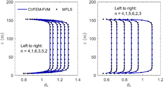
In this problem, six boreholes (diameter 𝑑𝑏 = 0.15 m) arranged in a 3 × 2 array at an angle of 𝛽𝑏= 30° relative to the direction of groundwater flow (as shown on Figure 2) are considered, and the heat flux on the outer surface of the boreholes is specified to be uniform and constant. Attention in this problem can thus be focused solely on the temperature and heat transfer in the groundwater-saturated soil of the borehole field, without dealing with the heat transfer and temperature of the boreholes and the working fluid flowing through the U-tube pipe within them. The dimensionless parameters considered in this problem are following: 𝐷𝑎 = 10−9, 𝛶 = 3, 𝛬 = 0.71, 𝜀 = 0.34; two values of the Peclet number 𝑃𝑒𝑑𝑏 = 0.01 and 𝑃𝑒𝑑𝑏 = 0.1; and on the outer surface of the active portions of the boreholes, (𝛶∇∗𝜃 ∙ 𝑛⃑ )
𝑏,𝑛= [𝑞𝑏,𝑛′′ (𝑧, 𝑡)/|𝑞̅̅̅̅̅] = 1 for 𝑏′′| {(𝐷/𝑑𝑏) ≤ 𝑧∗≤ {(𝐷 + 𝐻)/𝑑𝑏}. The calculation domain extends to 𝐿𝑊 = 𝐿𝐸 = 𝐿𝑁 = 𝐿𝑆 = 25 m on all sides of the borehole array in the horizontal plane; and 𝐻 = 150 m and 𝐿𝐵= 50 m (Fig. 1). The resulting total extents of the calculation domain are 𝐿𝑋 = 61.2 m,
34 𝐿𝑌 = 59.3 m and 𝐿𝑍 = 204 m. The total time of the simulations in this problem is 2 years (𝑡∗ = 395). The groundwater flow is assumed to be governed by the mathematical model presented in Section 3.2, and predicted using the CVFEM described in Section 4.1. The temperature and heat transfer in the groundwater-saturated soil are assumed to be governed by the mathematical model presented in Section 3.3, except for the prescription of a uniform and constant heat flux on the outer surface of each of the six boreholes, and predicted using the unsteady three-dimensional CVFEM-FVM described in Section 4.2. The spatial grid and time step used in the numerical solution of this problem were chosen using guidance from the baseline grid and time step discussed in the grid-independence study described in Section 5.1. The resulting grid consists of 354,660 pentahedral elements and is generated from a two-dimensional grid of 11,822 triangular elements.
A simplified version of this problem was also solved analytically using a moving-finite-line-source technique, which applies strictly only to the ground temperature around a line source, moving at a constant velocity and emitting heat uniformly along its length at a constant rate. Thus, the geometry considered in this moving-finite-line-source solution differs from the one considered in the numerical model, where heat is emitted from the impermeable cylindrical outer surfaces of the boreholes and the groundwater flows around them. Nonetheless, noting that the diameter of the boreholes is relatively small compared to the overall dimensions of the borehole field, a comparison of the numerical CVFEM-FVM predictions and the moving-finite-line-source analytical solution is provided in this section, as it provides a useful check or verification of the correct implementation of the numerical method.
A spatial superposition of the moving-finite-line-source analytical solutions gives the outer surface temperature of all six boreholes (n = 1 – 6):
35 𝑇̅𝑏,𝑘,𝑛(𝑡) = 𝑇𝑔+ ∑ ∑ 𝑑𝑏 2𝑘𝑠𝑞𝑏,𝑘𝑗,𝑎𝑐,𝑚 ′′ 𝑓 𝑘,𝑛,𝑘𝑗,𝑎𝑐,𝑚(𝑡) 𝑁𝑧,𝑎𝑐 𝑗=1 𝑁𝑏 𝑚=1 (38) 𝑓𝑘,𝑛,𝑘𝑗,𝑎𝑐,𝑚(𝑡) = 1 2Δz𝑘∫ 1 𝑠2𝐼 (𝑧𝑘𝑗,𝑎𝑐−1, Δ𝑧𝑘𝑗,𝑎𝑐, 𝑧𝑘−1, Δ𝑧𝑘) exp (−𝑠 2{(𝑑 𝑛,𝑚cos 𝛽𝑛,𝑚− ∞ 1 √4𝛼⁄ 𝑒𝑓𝑓𝑡 𝑣𝑇 4𝛼𝑒𝑓𝑓𝑠2) 2 + 𝑑𝑛,𝑚2 sin2𝛽𝑛,𝑚}) 𝑑𝑠 (39) 𝐼(𝑧𝑗−1, Δ𝑧𝑗, 𝑧𝑘−1, Δ𝑧𝑘) = erfint ((𝑧𝑘−1− 𝑧𝑗−1+ Δ𝑧𝑘)𝑠) − erfint ((𝑧𝑘−1− 𝑧𝑗−1)𝑠) + erfint ((𝑧𝑘−1− 𝑧𝑗−1− Δ𝑧𝑗)𝑠) − erfint ((𝑧𝑘−1− 𝑧𝑗−1+ Δ𝑧𝑘− Δ𝑧𝑗)𝑠) + erfint ((𝑧𝑘−1+ 𝑧𝑗−1+
Δ𝑧𝑘)𝑠) − erfint ((𝑧𝑘−1+ 𝑧𝑗−1)𝑠) + erfint ((𝑧𝑘−1+ 𝑧𝑗−1+ Δ𝑧𝑗)𝑠) − erfint ((𝑧𝑘−1+ 𝑧𝑗−1+
Δ𝑧𝑘+ Δ𝑧𝑗)𝑠) (40) erfint(𝑥) = ∫ erf(𝑥′) 𝑑𝑥′𝑥 0 = 𝑥 erf(𝑥) − 1 √𝜋(1 − exp(−𝑥 2)) (41)
In Eq. (39), 𝛼𝑒𝑓𝑓 = 𝑘𝑒𝑓𝑓⁄(𝜌𝑐𝑝)𝑒𝑓𝑓 is the effective thermal diffusivity of the groundwater-saturated soil; 𝑑𝑛,𝑚 = √(𝑥𝑏,𝑛− 𝑥𝑏,𝑚)
2
+ (𝑦𝑏,𝑛− 𝑦𝑏,𝑚)2 is the axial distance between boreholes 𝑛 and 𝑚 (it is set to 𝑑𝑛,𝑛= 𝑑𝑏⁄2 for 𝑛 = 𝑚); 𝛽𝑛,𝑚 = Arg (𝑥𝑏,𝑛− 𝑥𝑏,𝑚+ 𝑖(𝑦𝑏,𝑛− 𝑦𝑏,𝑚)) is the angle between boreholes 𝑛 and 𝑚 relative to the direction of flow (it is set to 𝛽𝑛,𝑛 = 𝜋 2⁄ for 𝑛 = 𝑚); and 𝑣𝑇 = 𝑈∞𝜌𝑤𝑐𝑝,𝑤 (𝜌𝑐𝑝)
𝑒𝑓𝑓
⁄ is an effective heat transport velocity. Eqs. (38) to (41) were obtained using the method of Claesson and Javed (2011), as elaborated in Cimmino and Bernier (2014), rather than the simplified moving-finite-line-source solution proposed by Tye-Gingras and Gosselin (2014) based on the method of Lamarche and Beauchamp (2007).
36 The outer-surface dimensionless temperatures (perimeter-average for the numerical results; denoted here as 𝜃𝑏) along the active length of the boreholes at 𝑡∗ = 395 are shown in Figure 6. The maximum difference between the numerical and analytical results for 𝜃𝑏 at the bottom of the active portion of the boreholes at 𝑡∗ = 395 is 5.16 % for 𝑃𝑒
𝑑𝑏 = 0.1; and at the mid-point of this portion, this maximum difference is 0.14 %. The time variations of the overall-average outer-surface dimensionless temperatures of the boreholes (denoted here as 𝜃̅𝑏) are shown in Figure 7. The maximum difference between the numerical and analytical results for 𝜃̅𝑏 at 𝑡∗= 395 is 0.23 % for 𝑃𝑒
𝑑𝑏 = 0.01; and it is 0.008 % for 𝑃𝑒𝑑𝑏 = 0.1.
Figure 6. Comparison of the numerical and analytical results for the axial variation of the
outer-surface dimensionless temperatures (perimeter-average for the numerical results; denoted here as