HAL Id: hal-03067235
https://hal.archives-ouvertes.fr/hal-03067235
Submitted on 23 Mar 2021
HAL is a multi-disciplinary open access archive for the deposit and dissemination of sci-entific research documents, whether they are pub-lished or not. The documents may come from teaching and research institutions in France or abroad, or from public or private research centers.
L’archive ouverte pluridisciplinaire HAL, est destinée au dépôt et à la diffusion de documents scientifiques de niveau recherche, publiés ou non, émanant des établissements d’enseignement et de recherche français ou étrangers, des laboratoires publics ou privés.
Design of a new device for fibers strand axial thermal
conductivity measurement
Baptiste Bouyer, Xavier Tardif, Célia Mercader, Didier Delaunay
To cite this version:
Baptiste Bouyer, Xavier Tardif, Célia Mercader, Didier Delaunay. Design of a new device for fibers strand axial thermal conductivity measurement. International Journal of Thermal Sciences, Elsevier, 2021, 161, pp.106740. �10.1016/j.ijthermalsci.2020.106740�. �hal-03067235�
1
Design of a new device for fibers strand axial
thermal conductivity measurement
Baptiste BOUYER1,2,*, Xavier TARDIF 2, Célia MERCADER 3, Didier DELAUNAY 1
¹ Université de Nantes, CNRS, Laboratoire de thermique et énergie de Nantes, LTeN, UMR 6607, F-44000 Nantes, France.
² Institut de Recherche Technologique (IRT) Jules Verne, 44340 Bouguenais, France
3 Plateforme CANOE, 33600 Pessac, France
ABSTRACT
A device for fibers strand axial thermal conductivity measurement has been designed and modelled by finite elements and realized. The method is based on Fourier's law in steady state and is inspired by the widely spread guarded hot plate method. This device has been designed to measure thermal conductivity on a wide range from 0.1 W/(m. K) to 100 W/(m. K) which represent the range of thermal conductivity found in fibrous materials. The numerical study has shown that radiative heat losses can reach the same order of magnitude than the researched conductive heat flux if no care is taken but are minimized when the temperature difference applied on the sample is centered on the temperature of the wall of the vacuum chamber enclosing the device. Measurements of thermal conductivity have been realized on three samples of bulk materials representative of the measurement range and on commercially available carbon fibers strands T300. The results are in good agreement with the values found in the literature and validate this device.
Keywords: Thermal conductivity, Measurement, Fibers strand, Guarded hot plate method, Numerical modeling, Design of experimental device.
* Corresponding author: baptiste.bouyer@univ-nantes.fr
2
1 INTRODUCTION
Fibers are used in many applications. They can be made of various materials, from natural origin, such as hemp or linen or synthetic such as glass or carbon fibers for the composite materials applications. The term fiber firstly indicates the morphology of the material: with a cylindrical shape and a micrometer diameter, and its ability to be woven. Depending on the nature of these fibers, the literature reports very low thermal conductivities from 0,06 W/(m. K)[1] for the most thermally insulating cellulose fibers, up to 520 W/(m. K)[2] for the most conductive carbon fibers. The fibers are often anisotropic and their longitudinal thermal conductivity might be greater than their transverse thermal conductivity by a factor of 1.5 to 50 [3]. The fibers, continuous or not, are gathered, and potentially twisted, to form strands. The effective thermal conductivity of fiber strands depends not only on fibers material but also on their morphology [4][5]: number, orientation (strand twisted or not ), continuity of fibers, etc. The effective thermal conductivity of fibers strands may be different of the thermal conductivity of individual fibers. Thus the thermal characterization of the strands is a critical step in the evaluation of the thermal properties of composite materials.
There are many methods for measuring the thermal conductivity of materials [6][7], and they are usually divided in two categories: The steady-state methods and the variable state methods: transient state or periodic state. The steady-state methods are usually based on the measurement of the unidirectional conductive heat flux passing through the sample and the temperature gradient induced in that direction in steady-state in order to determine the thermal resistance of the sample. Controlling and knowing the heat losses are thus essential to the precise determination of the conductive heat flux. Then the thermal conductivity is deduce from the thermal resistance what supposes to know the cross section of the sample. The heat flux measurement is direct in the case of absolute techniques and is the main challenge of the method [8][9] and indirect in the case of comparative techniques in which another material which thermal conductivity is known is used in series with the sample to be characterized to know the conductive heat flux passing through it [6]. In the variable state (transient and periodic) methods, the variation of the temperature of the sample periodically or punctually heated is measured in respect with the time and the compared to the corresponding analytical model. A curve fitting process is finally used to determine the thermal properties, often the thermal diffusivity, of the material. The thermal conductivity is deduced from the thermal diffusivity, what implies to know the thermal capacity and the density of the sample, which may lead to large uncertainties [10–12].
3
Some methods are suited for strands but most of the time the thermal characterization of fibers is limited to measurements of unidirectional composite materials [13] or microfibers. The thermal conductivity of fibers can be extracted from the composite material's one by using models of association of thermal resistances in series or parallel depending the direction considered or FEM analysis [3], what requires to know precisely the fiber content of the sample, the thermal conductivity of the matrix and the orientation of the fibers. Moses [13] used in this way the hot plate method to characterize carbon fibers with an accuracy of 10% after validating the method on a PTFE sample. Kawabata and Rengasamy [3] characterized many fibers with this method including T300 carbon fibers and obtained a longitudinal thermal conductivity of 6.72 W/(m. K) but did not indicate the measurement accuracy.
The thermal potentiometer is another steady-state method for the thermal conductivity measurement developed by Issi et al. in 1982 [14] and adapted for measurements on fiber strands over a temperature range of 4K to 100K for thermally insulating fibers and up to 300K for conductive fibers by Pirault, Issi and Coopmans in 1987 [15] [16]. The originality of the method lies in the compensation of heat loss by conduction in the sample supports and the thermocouple wires used to measure the temperature gradient in the sample, which makes it possible to measure the heat flow with good accuracy, the measurement being performed under vacuum to prevent convective heat loss. A thermal conductance (the inverse of the thermal resistance) of the sample is also defined by the authors according to the temperature of the measurement such that the radiation heat losses remain low compared to the conductive heat flux to guarantee an accuracy of 5%. This method has been used by Lavin et al.[17] to define a correlation between the thermal conductivity and the electrical resistance of the pitch-based carbon fibers.
In the "T-type probe" method developed by Zhang et al. [18], a metallic wire of known thermal and electrical conductivities is stretched between two thermo regulated electrodes at the same temperature. One end of the microfiber to be characterized is attached to the center of the wire while the other end is attached to a heat sink regulated at the same temperature as the electrodes, the assembly forming a "T". The device is placed in the chamber of a scanning electron microscope. The wire is heated by Joule effect with a direct current. The heat equation is solved in 1D steady state for both elements considered as thermally thin bodies. Thus, according to the authors, the temperature of the junction between the wire and the fiber depends solely on the thermal conductivities of the two elements, the heat flux generated in the wire and heat transfer coefficients between the wire or the fiber and the surrounding. The thermal
4
conductivity of the fiber is then deduced from the measurement of the heat flux generated and the average temperature of the wire. If measurements are possible on electrically insulating fibers, the method is insensitive to samples with low thermal conductivity. The authors validated the method with carbon fibers with a thermal conductivity greater than 120 W/(m. K) with an accuracy of 7%.
Very recently, Candalai et al. [19] presented an improved version of the "T-type probe" method for measuring the thermal conductivity of fiber strands in steady state. A wire, whose ends are held at a constant temperature, is heated by Joule effect. The heat generated passes into the sample which is placed perpendicular to the hot wire to form a cross. The ends of the sample are also kept at a constant temperature. The assembly is placed under vacuum to eliminate convective heat losses. The temperature fields obtained with and without the sample in contact with the hot wire are measured by high resolution infrared microscopy to determine the effective thermal conductivity of the strand using an associated analytical model. The authors take into account in their model the heat losses between the hot wire and the surrounding but neglect those between the sample and the surrounding. The method is validated with a Nichrome sample for which an accuracy of 10% is obtained, but no measurement is done on strands of thermally insulating fibers.
Among the transient methods, the flash method was adapted to microfibers by Demko et al. [20]: in a scanning electron microscope (SEM) a metallic micromanipulator provides instantaneous heating at one end of the fiber; the temperature response is then detected along the sample using a microfabricated sensor. The measurement of the variation of the electrical resistance of the sensor makes it possible to calculate the thermal diffusivity. Wu et al. [21] give a longitudinal thermal conductivity value of 7.9 W/(m. K) for T300 carbon fiber measured with the flash method, but do not specify either the experimental conditions or the accuracy of measurement. The flash method has also been adapted to fiber strands by Netzsch [22] but it requires a large amount of fibers (e.g. 35 meters of strands of 1000 fibers of 12.5 µm of diameter have been needed to make a sample) and is not suitable for semi-transparent fibers.
The mirage effect method was developed in particular by Barkoumb and Land [23] and by Sanchez-Lavega and Salazar [24][25]. The fiber to be characterized is heated locally by a low frequency modulated power laser (pump beam) to produce a synchronized thermal wave along the fiber. A second low power laser (probe beam) is directed perpendicularly to the fiber so as to barely touch the surface. The principle of the method consists in measuring the deflection of the probe beam due to the thermal gradient in the fluid surrounding the sample. The authors
5
perform several measurements by varying the distance between the two lasers to obtain an amplitude and phase profile that allows them to determine the conductivity and the thermal diffusivity of the sample. The major drawback of this technique is its difficulty of use, in particular the optical alignment of the laser beams, the detector and the fiber. In addition, this method only works for samples with a thermal diffusivity higher than 1 mm2/s.
The Angstrom method [26] [16] is at the origin of all known periodic-state methods. It consists in periodically heating one end of the sample made of carbon fiber strands by means of a heating element. The temperature of the sample is measured by thermocouples at two locations several centimeters apart. The phase shift obtained between the two measurements makes it possible to determine the thermal diffusivity of the sample. The measurement is carried out under vacuum to avoid heat losses by convection, however the method does not take into account heat losses by radiation. In addition, this method is reserved for fibers with a high thermal conductivity.
Mishra et al. [27] adapted the 3𝜔 method to the characterization of carbon microfibers. The microfiber is suspended between two thermo regulated metal electrodes at the same temperature. An alternative and sinusoidal electric current at the angular frequency 𝜔 heats by Joule effect the sample at the frequency 2𝜔. The change in temperature causes a variation in the electrical resistance which in turn produces a small change in voltage at a frequency of 3𝜔. The voltage variation at the angular frequency 3𝜔 is measured and compared with the corresponding analytical model. A curve fitting process makes it possible to simultaneously determine the longitudinal thermal conductivity of the sample as well as its volumic heat capacity. The authors perform measurements under vacuum to eliminate the convective heat losses, but do not specify the influence of radiative heat losses on the result. Thus this method is validated with a chromel wire with an accuracy of 8%. The authors also measured the longitudinal thermal conductivity of a T300 carbon fiber and obtained a value of 10 W/(m. K). To date, no measurements have been made with electrically and thermally insulating fibers.
A similar method, named "Direct Current Thermal Bridge Method (DCTBM)" developed by Moon et al. [28] takes the same experimental setup in steady state, also under vacuum. The sample is maintained at the temperature of the electrodes at the initial time and then heated by Joule effect by a continuous electric current. The temperature variation of the fiber is deduced from the variation of its electrical resistance. The temperature rise obtained in steady state allows the authors to determine the longitudinal thermal conductivity of the microfiber. The method has been validated by the authors with measurements on platinum and gold wires with
6
an accuracy of 11%. The measurement is also feasible on insulating fibers but requires to apply a platinum coating on the microfiber. A model makes it possible to determine the thermal conductivity of the fiber alone but requires precise knowledge of the conductivity and the thickness of the metal film, with the risk of significantly reducing the accuracy of the measurement. Newcomb et al. [29] used this method to characterize the longitudinal thermal conductivity of the T300 carbon fiber and obtain a value of 13.6 W/(m. K). Recently Jagueneau et al. [30] have improved this method by taking into account the heat losses by radiation in their analytical model and obtain an enhanced accuracy of 5%. Guo et al. [31] also use the same experimental setup, under the name "Transient Electrothermal Technique (TET)", but study the transient regime to determine the thermal diffusivity of the sample with an uncertainty of less than 10%.
The technique used by Yamane et al. [32], , the "AC Calorimetric method" also involves a local laser excitation to generate a thermal wave in the fiber to be characterized, however the authors study the thermal response of the fiber. Beyond a given distance from the excited zone, the heat transfer becomes unidirectional, the temperature is measured in that part by a thermocouple glued on the sample with silver lacquer. The study of the phase shift of the temperature in regards with the distance between the measurement and the excited zone (the laser can move along the fiber) makes it possible to determine the thermal diffusivity of the sample. Once again the measurement is carried out under vacuum to eliminate the heat losses by convection. The method is validated with samples of nickel and stainless steel, then used on carbon fibers, including a T300 carbon fiber for which the authors obtain a thermal conductivity of 5.9 W/(m. K) after measuring its density and its thermal capacity, however the authors do not indicate the accuracy of the measurement.
Pradere [33] and Pradere et al. [34] [10] have been inspired by the previous method and present a photothermal technique for measuring the thermal diffusivity of microfibers up to 2700K. The sample is first heated by Joule effect by a direct current to reach the desired temperature. Then, a local and periodical excitation is performed by a laser to obtain a thermal wave. The thermal response of the microfiber is measured by an infrared sensor that moves along the fiber. A curve fitting process applied to the experimental phase shift profile obtained allows the authors to determine the thermal diffusivity of the sample at the given temperature with estimated uncertainties of 5%.
Among the methods suitable for the measurement of the thermal conductivity of fibers presented above, only three can characterize fiber strands and are limited to thermally
7
conductive fibers. The other methods require the use of models to determine the thermal conductivity of the strands from the composite or the microfiber’s properties. Considering that the properties of the fiber strands depend also on their morphology and thus may differ from the properties of the microfibers that compose them, the development of a simple and direct method dedicated to the characterization of the longitudinal thermal conductivity of possibly low thermal conductivity fiber strands is relevant. We present here a new device designed to measure in steady state the effective longitudinal thermal conductivity of fiber strands over three orders of magnitude, from 0.1 W/(m. K) to 100 W/(m. K).
2 MATERIALS AND METHODS
2.1 Method principle
The method is inspired of the technique of the guarded hot plate based on the Fourier's law in one direction in steady state.
Where 𝑞⃗𝑐𝑜𝑛𝑑/(W/m2) is the heat flux density, 𝜅/(W/(m. K) is the thermal conductivity and ∇⃗⃗⃗𝑇/(K/m) is the temperature gradient. The conductive heat flux 𝑄𝑐𝑜𝑛𝑑 passing through the sample is then given by integrating the heat flux density over the constant cross section A, leading to the following expression:
Where R is the thermal resistance of the sample. Generally the sample is a plate submitted to a unidirectional temperature gradient and the device lateral surfaces are thermally insulated in order to make the lateral heat losses negligible. The heat is dissipated by an electrical resistance and a hot guard ensures the heat passes solely in the sample. The determination of the thermal conductivity 𝜅 then lies on the measurement of the temperature difference 𝛥𝑇 between the faces of the sample separated by a distance 𝐿 and the measure of the conductive heat flux 𝑄𝑐𝑜𝑛𝑑 passing through the sample. The conductive heat flux is equal to the electrical power dissipated by the heating element 𝑄𝑒𝑙𝑒𝑐 if the heat losses 𝑄losses are neglected. The system is then described by the following equations:
𝑞⃗𝑐𝑜𝑛𝑑 = −𝜅𝛻⃗⃗𝑇 (1)
𝑄𝑐𝑜𝑛𝑑 = ∬ 𝑞⃗𝑐𝑜𝑛𝑑 . 𝑑𝐴⃗⃗⃗⃗⃗⃗ 𝐴
8
𝑅 = 𝛥𝑇 𝑄⁄ 𝑐𝑜𝑛𝑑 ≅ 𝛥𝑇 𝑄⁄ 𝑒𝑙𝑒𝑐 (4)
With 𝑄losses the lateral convective and radiative heat transfers between the sample and the surrounding. Most of the measurement errors linked to this method comes from those heat losses. The thermal conductivity of the sample is deduced from the thermal resistance knowing the dimensions of the sample:
In the case of the guarded hot plate adapted to fibers strands, the sample is made of few aligned fiber strands with a length of 150 or 200 millimeters, each strand being composed by thousands of fibers (generally 1000 (1k), 3000 (3k), 6000(6k) or 12 000 (12k)), twisted or not, of few micrometers of diameter. Therefore, the lateral surface of the sample is much larger than its cross section, consequently a particular attention should be taken to the heat losses in this device. To avoid heat losses by convection, the measurements are done under vacuum. Consequently, the presented device might be not be suited for strands made of low conductivity porous fibers with interstitial fluid.
2.2 Computer assisted design of the experimental device
The device has been designed by FEM analysis with the software COMSOL Multiphysics® to minimize the heat losses by radiation between the sample and the surrounding. The use of radiative shield, the influence of the surrounding temperature and finally the influence of the sample length have been particularly studied. The device is supposed to be placed in a vacuum chamber with thermo-regulated walls to avoid convective heat losses and to control the surrounding temperature.
A scheme of the device is represented in the Figure 1. The sample (2) is held vertically between the heating system (1) and the cooling system (4) in a way that the strands are tensioned. The heating system (1) is composed of two heating resistors (1.1) whose electrical power consumption is measured and between which the sample (2) is held. This part is thermally insulated with a foam (1.2) with a thermal conductivity of 0.03 W/(m. K). The whole is surrounded by the hot guard (1.3) composed of heat exchangers in copper in which
𝑄𝑒𝑙𝑒𝑐 = 𝑉𝐼 = 𝑄𝑐𝑜𝑛𝑑+ 𝑄𝑙𝑜𝑠𝑠𝑒𝑠 (3)
9
flows thermo-regulated water at the temperature 𝑇𝐻𝑜𝑡. The cooling system (4) is also made of heat exchangers in copper in which flows thermo-regulated water but at the temperature 𝑇𝐶𝑜𝑙𝑑, sort as 𝑇𝐻𝑜𝑡 is greater than 𝑇𝐶𝑜𝑙𝑑.
The radiative shield (3) that has been designed is fixed to the cooling and heating systems and surrounds the sample. The radiative shield retained is made of insulating foam (3.1) and aluminum sheet (3.2) and only the surfaces of the shield facing the sample are coated with the aluminum sheet.
2.2.1 Numerical modeling
The entire device shown in Figure 1, vacuum chamber included, is modeled by finite elements. The three-dimensional heat equation used in each domain of the model is the following:
10 𝜌𝑐𝜕𝑇 𝜕𝑡 = 𝜕 𝜕𝑥(𝜅𝑥 𝜕𝑇 𝜕𝑥 ) + 𝜕 𝜕𝑦(𝜅𝑦 𝜕𝑇 𝜕𝑦 ) + 𝜕 𝜕𝑧(𝜅𝑧 𝜕𝑇 𝜕𝑧 ) (6)
Where 𝜌/(kg/m3) is the density, 𝑐/(J/(kg. K)) is the thermal capacity at constant pressure and 𝜅/(W/(m. K)) is the thermal conductivity of the material of the considered domain. The thermal contact resistances between the sample and the heating and the cooling systems are neglected so as the heat losses in the wires of the heating resistances and thermocouples. The modeled sample is a PMMA strip 200 mm long, 20 mm wide and 1.5 mm thick. The thermal conductivity of PMMA set in the model is 0.18 W/(m. K). This sample will then be used as a standard to characterize the experimental setup.
The following boundary conditions have been used in the numerical model:
- Imposed temperature on the external wall of the vacuum chamber:
𝑇 = 𝑇𝑤𝑎𝑙𝑙 (7)
- Convective heat flux on the walls of the channels of the heat exchangers:
𝜑𝑐𝑜𝑛𝑣 = ℎ(𝑇 − 𝑇∞) (8)
𝑇∞ is the fluid temperature respectively 𝑇𝐻𝑜𝑡 or 𝑇𝐶𝑜𝑙𝑑. The heat exchange coefficient h is calculated considering the geometry and the flow rate using the classical Colburn correlation for a short tube [35]:
ℎ = (𝑁𝑢𝐷,𝐿∗ 𝜅𝑤𝑎𝑡𝑒𝑟) 𝐷⁄ (9)
𝑁𝑢𝐷,𝐿 = 𝑁𝑢𝐷,∞ [1 + (𝐷 𝐿⁄ )0.7] (10)
11
The exchange coefficient h is found to be equal to 3653 W/(m2. K) for all channels, with a Prandtl number 𝑃𝑟 = 7 and a Reynolds number 𝑅𝑒𝐷 = 5090.
- All free surfaces of the device as well as the inside surfaces of the vacuum chamber are considered to be diffusive surfaces: two free surfaces at different temperatures facing each other exchange heat by radiation. The radiative heat flux from the surface element i to the surface element j is written :
𝑞𝑟𝑎𝑑,𝑖→𝑗 = 𝜎𝔉𝑖→𝑗(𝑇𝑖4− 𝑇𝑗4) (12) With 𝔉𝑖→𝑗 = 1 𝜌𝑖 𝜖𝑖(1 − τi)+ 1 𝐹𝑖→𝑗(1 − 𝜏i )(1 − 𝜏𝑗)+ 𝜌𝑗 𝜖𝑗(1 − 𝜏𝑗)∗ 𝐴𝑖 𝐴𝑗 (13)
Where 𝜎/(W/(m2 . K4 )) is the Stefan-Boltzmann constant and 𝜖𝑖, 𝜌𝑖, 𝜏𝑖 are the radiative properties, respectively emissivity, reflectance and transmittance, of the material of the surface element 𝑖 of area 𝐴𝑖 and 𝐹𝑖→𝑗 is the shape factor between the surface elements 𝑖 and 𝑗. The shape factors are determined by the hemi-cube method [36] with a resolution of 512. For a surface element 𝑖 of the mesh belonging to a diffusive surface, the surrounding is projected onto a hemi-cube centered on the surface element 𝑖. A resolution of 512 means that each face of the hemi-cube is discretized into 512² pixels. The fraction of the pixels covered by the projection of a surface element 𝑗 onto the hemi-cube leads to the shape factor from surface element 𝑗 to surface element 𝑖. This process is repeated for each surface element of the model belonging to a diffuse surface to obtain a complete set of shape factors. Thus radiative heat transfers between all diffuse surfaces seeing each other are taken into account. The radiative properties of each materials are previously measured at the laboratory using a FTIR spectrometer Bruker Vertex 80V.
- As initial condition, the whole model is at the temperature imposed on the wall of the vacuum chamber :
12
The mesh consists of 189,952 tetrahedral elements. The quality of an element is defined as the ratio between the largest and the smallest dimension of the element. The average quality of the mesh elements is 0.66. The 3D model, the vacuum chamber excepted, is represented on the Figure 2.
2.2.2 Numerical results
The simulations have been performed in steady state, in conformity with the experiment. For each simulation, the cooling and heating systems temperatures have been set respectively to 20°C and 30°C. The use of the radiative shield, different wall temperatures and various sample lengths have been tested. The simulations setups (i.e. the use of the shield, the wall temperature, the effective sample length, the cross section A along the direction 𝑧⃗ and the lateral surface) and their results are reported in the Table 1. As results, the reader will find the theoretical conductive heat flux given by the equation (2), the numerical conductive heat flux in the three directions (volume-averaged conductive heat flux density multiplied by the sample cross section along the considered direction), the radiative heat flux (integrated over the lateral surface of the sample) and the ratios between the conductive heat flux along 𝑥⃗ and 𝑦⃗ directions and the 𝑧⃗ direction, the numerical and theoretical conductive heat flux along the 𝑧⃗ direction and finally the ratio between radiative heat flux and conductive heat flux along the 𝑧⃗ direction. The difference between the temperature distributions along 𝑧⃗ in the sample from the simulations and from analytical solution obtained by neglecting the heat losses, mentioned as “theory” are
13
represented in the Figure 3. A positive difference indicates that the sample receives heat by radiation, in the contrary a negative one shows heat losses by radiation.
Simulation number #1 #2 #3 #4 #5 #6
Radiative shield No Yes Yes Yes Yes Yes
Twall /°C 25 25 20 30 25 25 Leff sample /mm 190 190 190 190 140 90 A /mm² 30 30 30 30 30 30 Slateral /mm² 8170 8170 8170 8170 6020 3870 Qcond z theo /W -2.84×10 -4 -2.84×10 -4 -2.84×10 -4 -2.84×10 -4 -3.86×10 -4 -6.00×10 -4 Qcond x num /W Qcond y num /W Qcond z num /W -4.40×10 -8 -3.27×10 -6 -3.10×10 -7 -3.52×10 -7 1.12×10 -7 -1.99×10 -6 4.32×10 -5 4.39×10 -6 7.60×10 -6 7.28×10 -6 2.23×10 -6 3.25×10 -6 -2.78×10 -4 -2.80×10 -4 -2.83×10 -4 -2.83×10 -4 -3.81×10 -4 -5.89×10 -4 Qrad, num /W 2.59×10 -4 8.71×10 -6 -5.74×10 -4 5.61×10 -4 2.21×10 -5 5.47×10 -5
|Qcond x num / Qcond z num| 0.0% 1.2% 0.1% 0.1% 0.0% 0.3%
|Qcond y num / Qcond z num| 16% 1.6% 2.7% 2.6% 0.6% 0.6%
|Qcond z num / Qcond z theo| 98% 98.4% 99.6% 99.4% 98.7% 98.2%
|Qrad num / Qcond z num| 93% 3.1% 203% 198% 5.8% 9.3%
Table 1: Numerical simulations of the device: set up and results.
Figure 3: Temperature difference between the simulations results and the tempereature obtained by neglecting the radiative heat transfer.
14
A first comparison can be done between the simulation #1 and #2 to evaluate the impact of the radiative shield. The temperature fields obtained in both of the cases are represented in the Figure 4. It can be noticed that without the radiative shield the sample temperature distribution does not follow the unidirectional linear temperature gradient between the heating and the cooling systems expected but almost all the sample is at the wall temperature and large temperature gradients are found at the ends of the sample. Moreover the ratio of 16% between the conductive heat flux between the 𝑦⃗ and 𝑧⃗ directions presented in the Table 1 show that the conductive heat flux cannot be considered as unidirectional. These results show that radiative heat losses between the sample and the wall of the vacuum chamber are not negligible without radiative shield. However, the temperature field obtained with the radiative shield is closer to the one expected: the side of the shield in regards with the wall of the vacuum chamber is made of very insulating materials and the sample side of the shield is made of aluminum which is very conductive and has low emissivity. The conductive part of the radiative shield being in contact with the heating and the cooling systems, the aluminum part of the shield follows the linear temperature gradient expected in the sample thus at a given height, the shield and the sample have very close temperature, limiting the radiative heat transfer to 3% of the conductive heat transfer which can be considered as unidirectional since the conductive heat flux along 𝑥⃗ and 𝑦⃗ represent respectively 1.2% and 1.6% of the conductive heat flux along 𝑧⃗ .
Figure 4: Numerical simulations results: temperature field in the device without the radiative shield (a) and with the radiative shield (b).
15
In simulations #2, #3 and 4#, the wall temperature is set respectively up to 25°C, 20°C and 30°C to study its effect on the sample temperature distribution. The ratios between the radiative heat flux and the vertical conductive heat flux in the Table 1 show that the wall temperature has to be equal to the average value of the hot and cold temperatures, imposed respectively at the heating and cooling systems, to minimize the radiative heat transfer as suggested for instance in [37,38]. When the wall temperature is equal to one of the heating or cooling system, the intensity of radiative heat flux can reach as much as twice the conductive heat flux for samples with low thermal conductivity. This can be explain by analyzing the Figure 3: in simulation #3 and #4, the difference is negative, respectively positive, along all the sample resulting in losing heat, respectively gaining heat, by radiation when integrating over all the lateral surface of the sample. However, in simulation #2, the difference is positive in the first half of the sample and then negative in a symmetrical way, leading to a compensation of the heat loss and gain when integrating the radiative heat transfer over the lateral surface of the sample.
The comparison between simulation #2, #5 and #6 finally show the effect of the sample length: by decreasing the sample length the thermal resistance of the sample decreases as well leading to an increase of the conductive heat flux. In the same time the radiative heat flux increases too which can be attributed to the edges effect (see figure 3): decreasing the sample length leads to the increase of the relative area of radiative heat transfer, i.e. the geometrical shape factor, between the heating and the cooling systems and the sample and thus to an increase of the heat gain and heat losses at the ends of the sample. The materials of the heating and the cooling systems being different, the emissivity of the surfaces are different too, the heat gain and loss do not compensate each other and thus the ratio between radiative heat flux and conductive heat flux increases. A long sample is then preferable.
A longer sample is also advantageous for others reasons: it allows an easier and more precise thermal instrumentation of the sample since the temperature gradient is lower and thus the temperature measurement less sensitive to the location of the sensors such as thermocouples.
Finally, a bigger thermal resistance of the sample makes the contact resistances, which do not depend on the sample length, relatively lower and thus helps to neglect them. Measurements will be done on samples with different length in the part 3 to ensure that the contact resistances do not affect the result.
16 2.2.3 Numerical validation of the device
Further numerical simulations modeling the measurements on fibers strands have been realized with small cross section samples, various temperature differences between the heating and the cooling systems and several values for the thermal conductivity of the sample from 0.1 to 100 W/(m.K). A cross section of 1.7mm² represents a sample made of 10 fibers strands containing 6000 fibers of 6µm diameter. Likewise, cross sections of 8.5mm² and 13.6mm² represent samples made of 50 fibers strands and 80 fibers strands respectively.
For each simulation, the theoretical conductive heat flux given by the equation (2) (𝑄𝑐𝑜𝑛𝑑 𝑡ℎ𝑒𝑜), the numerical conductive heat flux in the z direction (𝑄𝑐𝑜𝑛𝑑 𝑧), the radiative heat flux (integrated over the lateral surface of the sample) (𝑄𝑟𝑎𝑑) and the heat losses by conduction between the heating resistances and the guard within the heating system (𝑄𝑙𝑜𝑠𝑠) are calculated and reported in Table 2 as well as the ratios between 𝑄𝑟𝑎𝑑 and 𝑄𝑐𝑜𝑛𝑑 𝑧 and between 𝑄𝑙𝑜𝑠𝑠 and 𝑄𝑐𝑜𝑛𝑑 𝑧. 𝜅 W/(m.K) 𝛥𝑇 K 𝐴 mm² 𝑄𝑐𝑜𝑛𝑑 𝑡ℎ𝑒𝑜 W 𝑄𝑐𝑜𝑛𝑑 𝑧 W 𝑄𝑟𝑎𝑑 W 𝑄𝑙𝑜𝑠𝑠 W 𝑄𝑟𝑎𝑑 / 𝑄𝑐𝑜𝑛𝑑 𝑧 𝑄𝑙𝑜𝑠𝑠/ 𝑄𝑐𝑜𝑛𝑑 𝑧 0.1 10 1.7 8.50 10−6 8.49 10−6 1.50 10−6 3.93 10−7 17.64% 4.63% 0.1 40 13.6 2.72 10−4 2.72 10−4 5.15 10−6 6.08 10−6 1.90% 2.24% 1 10 1.7 8.50 10−5 8.49 10−5 3.55 10−6 1.59 10−6 4.19% 1.87% 1 30 8.5 1.28 10−3 1.27 10−3 8.26 10−6 1.56 10−5 0.65% 1.23% 10 10 1.7 8.50 10−4 8.49 10−4 5.25 10−6 8.63 10−6 0.62% 1.02% 10 20 1.7 1.70 10−3 1.70 10−3 8.29 10−6 1.75 10−5 0.49% 1.03% 100 10 1.7 8.50 10−3 8.49 10−3 5.41 10−6 6.63 10−5 0.06% 0.78%
For each case, it can be noticed that the theoretical conductive heat flux and the numerical conductive heat flux are very close. For given temperature difference and cross section, the heat losses by radiations and by conduction between the heating resistances and the guard rise with the thermal conductivity of the sample.
Ratios between heat losses and heat flux by conduction show that for low thermal conductivity samples (𝑘 ≤ 1 𝑊/(𝑚. 𝐾)) with a temperature difference of 10K and a cross section of 1.7mm² (10 fibers strands) the heat losses cannot be considered as negligible. However, by setting a bigger temperature difference and using a larger sample (made with more fibers strands), the conductive heat flux rises, as well the heat losses, and ratios between heat
17
losses and conductive heat flux are reduced to acceptable values (sum of heat losses less than 5%).
For high thermal conductivity samples (𝑘 ≥ 10𝑊/(𝑚. 𝐾)), heat losses can be neglected for a temperature difference of 10K and a sample made of 10 fibers strands.
The device is therefore numerically validated over the full measurement range required, from 0.1W/(m.K) to 100W/(m.K) for the fibers strands axial thermal conductivity measurement provided that the number of fibers strands and temperature difference lead to sufficient heat flux by conduction passing through the sample.
3 EXPERIMENTAL VALIDATION OF THE DEVICE 3.1 Experimental device and measurements
The device has been machined and is shown in the Figure 5. The different temperatures are measured with K type thermocouples.
The device is placed in a vacuum chamber, under primary vacuum at 10−4 mbar to avoid convective heat losses. The temperature of the walls of the vacuum chamber is regulated at the temperature 𝑇𝑤𝑎𝑙𝑙 by inner channels in which flows thermo-regulated water to control the surrounding. The thermo-regulated water flowing in the different parts of the device is provided by external thermostatically-controlled water baths with their own PID controller.
18
Each heating resistance (1.1) presents an electrical resistance of 60,3Ω. The resistances are connected in parallel to a direct current source Keithley 6221 piloted by a PID controller.
The parameters of the PID controller are evaluated before each measurement. The PID controller and the temperatures acquisition system have been realized by using the software LabVIEW™ (National Instrument Corp.)
The heating resistances are controlled so as the temperature difference Δ𝑇𝑐𝑜𝑛𝑡𝑟𝑜𝑙, measured between the heating resistance and the hot guard (see Figure 1) goes below 0.01K. When the steady state is reached, the heat flux passing through the sample corresponds to the heat dissipated by the heating resistances given by their electrical consumption. The cross section of the sample, given by the number of fibers strands, and the temperature difference between the heating and the cooling systems must be chosen to ensure a conductive heat flux greater than 1.10−3𝑊 to ensure that the conductive heat flux between the heating element and the hot plate remains less than 5% of the heat flux passing through the sample. For instance, to measure the thermal conductivity of fibers strands containing 1000 fibers of 13µm diameter and with a thermal conductivity of 1 W/(m.K), the sample should be made of 60 fibers strands for a temperature difference of 30K between the heating and the cooling systems. The thermal conductivity is then obtain by the following expression coming from the equations (4) and (5):
𝜅 =Q 𝐴∗
𝐿
𝛥𝑇 (15)
Or in this case for a rectangular cross section sample of thickness 𝑡/(m) and width 𝑤/(m):
𝜅 = 𝑉𝐼 𝑡 ∗ 𝑤∗
𝐿
𝑇𝐻𝑜𝑡− 𝑇𝐶𝑜𝑙𝑑 (16)
Where 𝑉/(V) is the voltage measured over the resistances, 𝐼/(A) is the electrical current intensity delivered by the current source and 𝐿/(m) is the effective length of the sample which is the distance between the heating system and the cooling system (cf. Figure 1). The quantities measured at steady state, electrical voltage, electrical intensity and temperatures correspond to an average value obtained over a period of 1000 seconds, with an acquisition frequency of 1 Hz.
19
The relative uncertainty of the thermal conductivity obtained is then given by the following expression: Δ𝜅 𝜅 = Δ𝑉 𝑉 + Δ𝐼 𝐼 + Δ𝐴 𝐴 + Δ𝐿 𝐿 + ΔTHot+ Δ𝑇𝐶𝑜𝑙𝑑 𝑇𝐻𝑜𝑡− 𝑇𝐶𝑜𝑙𝑑 (17)
Where each of the terms is to be minimized to increase the accuracy of the obtained thermal conductivity. The uncertainty of the temperature measurement can further be minimized by increasing the temperature difference applied to the sample. The uncertainties of the average quantities are obtained by the standard deviation of the measurement series.
3.2 Experimental validation with bulk materials samples
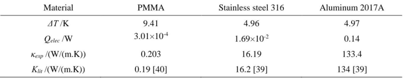
Measurements have been realized on three samples of bulk materials representative of the range of thermal conductivity required. The first one is a strip of PMMA of dimensions 1.5mm x 20mm x 200mm, the second one a strip of stainless steel 316 of dimensions 2mm x 20mm x 200mm and the third one is a strip of aluminum 2017A with the same size as the second sample. For the PMMA, a temperature difference of 10K is applied to the sample, while for the second and third samples a difference of only 5K is applied to limit the heat flux, the current source used being limited at 100mA. Special attention is paid to the control of the temperature of the wall of the vacuum chamber, to be equal to the average of the temperatures of the heating and cooling systems. The measured temperature difference, the electrical power consumed by the heating resistances and the thermal conductivity obtained are presented for each sample in the Table 3. The thermal conductivity obtained experimentally 𝜅𝑒𝑥𝑝 is compared with the thermal conductivity of the corresponding material found in the literature [39,40] 𝜅𝑙𝑖𝑡. The thermal conductivity of PMMA is extracted from reference [40]. It depends on how the sample is obtained (molded or extruded) but an average value of 0.19 ± 0.01 W/(m. K) can be retained.
Material PMMA Stainless steel 316 Aluminum 2017A
ΔT /K 9.41 4.96 4.97 Qelec /W 3.01×10 -4 1.69×10⁻² 0.14 κexp /(W/(m.K)) 0.203 16.19 133.4 Κlit /(W/(m.K)) 0.19 [40] 16.2 [39] 134 [39]
20
A very good agreement with the values found in the literature is obtained for the metal samples. A larger relative difference is obtained for the less heat conducting sample, as might be expected, since the radiative losses are relatively greater compared to the conductive heat flux that passes through the sample. Nevertheless, the values obtained validate the device and the method over the entire measurement range required.
3.3 Experimental validation with fibers strands samples
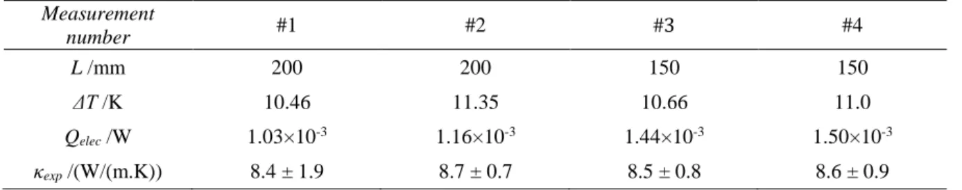
The device being validated on bulk samples, measurements have been then performed on Toray T300 commercial carbon fiber samples. Four measurements were made on four different samples consisting of 10 strands of 6000 carbon filaments of 6 µm of diameter. The length of the samples, the temperature difference applied to the sample, the measured electrical power consumed by the heating resistances and the axial thermal conductivity obtained for each of the measurements are indicated in the Table 4. Samples with two different lengths have been tested to ensure that thermal contact resistances between the heating and cooling systems and the sample are negligible. Results show that the thermal conductivity does not change with the sample length and confirm that the thermal contact resistances are insignificant.
The obtained results are shown in the Figure 6 and compared to the axial thermal conductivities of T300 carbon fibers found in the literature. Of the twelve references found, six [41][42][43][44][45][46] do not specify how the thermal conductivity was obtained and announce 8, 10.5, 8.5, 7, 8.5 and 9.4 W/(mK), respectively. These references are manufacturer's data or article citing manufacturer's data. The other values were obtained with different methods: Yamane et al. [32] obtain a thermal conductivity of 5.9𝑊/(𝑚. 𝐾) with the previously mentioned AC calorimetric method. Kawabata et al. [3] have deduce the thermal conductivity of T300 carbon fibers from the characterization of a composite material with the guarded hot plate technique, knowing the thermal properties of the matrix, leading to a value of 6.72 W/(m.K) while Wu et al. [21] use a thermal conductivity value of 7.9 W/(m. K)
Measurement number #1 #2 #3 #4 L /mm 200 200 150 150 ΔT /K 10.46 11.35 10.66 11.0 Qelec /W 1.03×10⁻³ 1.16×10⁻³ 1.44×10⁻³ 1.50×10⁻³ κexp /(W/(m.K)) 8.4 ± 1.9 8.7 ± 0.7 8.5 ± 0.8 8.6 ± 0.9
21
obtained with the flash method. Villière et al. [47] consider an average value between several values found in the literature and thus announces a thermal conductivity of 8.8 W/(m. K). Newcomb et al. [29] obtain 13.6 W/(m. K) with the DC Thermal Bridge method and finally Mishra et al. [27] measure 10 W/(m. K) with the 3𝜔 method. The thermal conductivities obtained experimentally with the new device are between 8.4 W/(mK) and 8.7 W/(mK) and are therefore in very good agreement with the literature (mean value of 8.69W/(mK)), which validates the use of this new device for the fibers axial thermal conductivity measurement.
4 CONCLUSION
A device for axial thermal conductivity measurement of strands of fiber inspired by the guarded hot plate method has been developed and modeled by finite elements to estimate the heat losses by radiation.
The numerical model has shown that radiative heat losses are minimized if the temperature difference applied to the sample is centered on the wall temperature of the vacuum chamber. Then, the numerical model have been used to numerically validate this new device over the full measurement range required, from 0.1W/(m.K) to 100W/(m.K) for the fibers strands axial thermal conductivity measurement.
22
Experimental measurements have been performed on three standard samples of bulk materials representative of the measuring range of the device: a sample of PMMA of low thermal conductivity, a sample of aluminum of high thermal conductivity and a sample of stainless steel of intermediate thermal conductivity. The values obtained are very close to the one found in the literature.
Then measurements have been performed on fibers samples. The samples are made of commercial carbon fibers strands T300. The given results are compared once more to the literature and show a very good agreement.
This new device is experimentally validated on the range 0.2 to 100𝑊/(𝑚. 𝐾) for large cross section samples (30mm²) and for fibers strands such as the heat flux passing through the sample is greater than 1.10−3W. This implies to adjust the setting temperatures and the size of the sample (length and number of fibers strands) to reach the adequate thermal resistance.
ACKNOWLEDGEMENTS
In the first hand, we would like to thank Nicolas Lefevre for the relevance of his remarks and in other hand Arnaux Arrivé and Julien Aubril for their involvement in the realization of this device, the three of them working for the studies and manufacturing department of the LTeN.
This work is part of the FORCE project managed by IRT Jules Verne (French Institute in Research and Technology in Advanced Manufacturing Technologies for Composite, Metallic and Hybrid Structures)
23 NOMENCLATURE
Symbols
A: cross section area
c : thermal capacity
D : diameter
I: electrical current intensity L: length
Nu: Nusselt number
𝑃𝑒𝑙𝑒𝑐: electrical power
Pr: Prandtl number R: thermal résistance Re: Reynolds number T: temperature t: thickness 𝑉: electrical voltage w: width Greek letters Δ: Difference
𝜖𝑖, 𝜌𝑖, 𝜏𝑖 : emissivity, reflectance, transmittance of surface 𝑖 𝑄 : heat flux
𝑞: heat flux density 𝜅 : thermal conductivity 𝜌 : density
24 REFERENCES
[1] S. Binet, S. Malard, M. Ricaud, A. Romero-Hariot, B. Savary, Fibres de cellulose, Base de Données Fiches Toxicologiques INRS. (2011).
[2] G. Dupupet, Fibres de carbone, Techniques de l’ingénieur. (2008) 1–19.
[3] S. Kawabata, R.S. Rengasamy, Thermal conductivity of unidirectional fibre composites made from yarns and computation of thermal conductivity of yarns, Indian Journal of
Fibre & Textile Research. 27 (2002) 217–223.
http://nopr.niscair.res.in/handle/123456789/22853 (accessed September 20, 2019). [4] R.S. Rengasamy, S. Kawabata, Computation of thermal conductivity of fibre from
thermal conductivity of twisted yarn, Indian Journal of Fibre & Textile Research. 27 (2002) 342–345. http://nopr.niscair.res.in/bitstream/123456789/23185/1/IJFTR 27(4) 342-345.pdf (accessed October 3, 2019).
[5] F. Fayala, H. Alibi, A. Jemni, X. Zeng, Study the effect of operating parameters and intrinsic features of yarn and fabric on thermal conductivity of stretch knitted fabrics using artificial intelligence system, Fibers and Polymers. 15 (2014) 855–864. https://doi.org/10.1007/s12221-014-0855-y.
[6] D. Zhao, X. Qian, X. Gu, S. Ayub Jajja, R. Yang, Measurement Techniques for Thermal Conductivity and Interfacial Thermal Conductance of Bulk and Thin Film Materials, Journal of Electronic Packaging. 138 (2016) 040802. https://doi.org/10.1115/1.4034605. [7] M. Thomas, Propriétés thermiques de matériaux composites : caractérisation
expérimentale et approche microstructurale, Université de Nantes, Nantes, Fr, 2008. [8] R. Le Goff, D. Delaunay, N. Boyard, V. Sobotka, Thermal conductivity of an injected
polymer and short glass fibers composite part: measurement and model, in: 27th World Congress of the Polymer Processing Society, Marrakech, Morocco, 2011: pp. 2357– 2363.
[9] W.C. Thomas, R.R. Zarr, Thermal response simulation for tuning PID controllers in a 1016 mm guarded hot plate apparatus, ISA Transactions. 50 (2011) 504–512. https://doi.org/https://doi.org/10.1016/j.isatra.2011.02.001.
[10] C. Pradere, J.-C. Batsale, J.-M. Goyhénèche, R. Pailler, S. Dilhaire, Thermal properties of carbon fibers at very high temperature, Carbon. 47 (2009) 737–743. https://doi.org/10.1016/J.CARBON.2008.11.015.
[11] J. Guo, X. Wang, D.B. Geohegan, G. Eres, C. Vincent, Development of pulsed laser-assisted thermal relaxation technique for thermal characterization of microscale wires,
25
Journal of Applied Physics. 103 (2008). https://doi.org/10.1063/1.2936873.
[12] H. Brendel, G. Seifert, F.G. Raether, Determination of thermal diffusivity of fibrous insulating materials at high temperatures by thermal wave analysis, International Journal
of Heat and Mass Transfer. 108 (2017) 2514–2522.
https://doi.org/10.1016/j.ijheatmasstransfer.2017.01.063.
[13] W.M. Moses, Measurement of Thermal Conductivity of PAN Based Carbon Fiber, Georgia Institute of Technology, 1978.
[14] J.-P. Issi, J. Boxus, B. Poulaert, J.P. Heremans, Thermopower and thermal conductivity measurements on intercalation compounds., in: Thermal Conductivity, Plenum Press, 1983: pp. 537–544. https://doi.org/10.1007/978-1-4899-5436-7_50.
[15] L. Piraux, J.-P. Issi, P. Coopmans, Apparatus for thermal conductivity measurements of thin fibres, Measurement. 5 (1987) 2–5.
[16] N.C. Gallego, D.D. Edie, B. Nysten, J.-P. Issi, J.W. Treleaven, G. V. Deshpande, Thermal conductivity of ribbon-shaped carbon fibers, Carbon. 38 (2000) 1003–1010. https://doi.org/10.1016/S0008-6223(99)00203-1.
[17] J.G. Lavin, D.R. Boyington, J. Lahijani, B. Nysten, J.-P. Issi, The correlation of thermal conductivity with electrical resistivity in mesophase pitch-based carbon fiber, Carbon. 31 (1993) 1001–1002. https://doi.org/https://doi.org/10.1016/0008-6223(93)90207-Q. [18] X. Zhang, S. Fujiwara, M. Fujii, Measurements of Thermal Conductivity and Electrical
Conductivity of a Single Carbon Fiber, International Journal of Thermophysics. 21 (2000) 965–980. https://doi.org/https://doi.org/10.1023/A:1006674510648.
[19] A.A. Candadai, J.A. Weibel, A.M. Marconnet, A Measurement Technique for Thermal Conductivity Characterization of Ultra-High Molecular Weight Polyethylene Yarns Using High-Resolution Infrared Microscopy, in: 2019 18th IEEE Intersociety Conference on Thermal and Thermomechanical Phenomena in Electronic Systems
(ITherm), IEEE, Las Vegas, 2019: pp. 490–497.
https://doi.org/10.1109/ITHERM.2019.8757385.
[20] M.T. Demko, Z. Dai, H. Yan, W.P. King, M. Cakmak, A.R. Abramson, Application of the thermal flash technique for low thermal diffusivity micro/nanofibers, Review of Scientific Instruments. 80 (2009) 1–3. https://doi.org/10.1063/1.3086310͔.
[21] G.-P. Wu, D.-H. Li, Y. Yang, C.-X. Lu, S.-C. Zhang, X.-T. Li, Z.-H. Feng, Z.-H. Li, Carbon layer structures and thermal conductivity of graphitized carbon fibers, Journal of Materials Science. 47 (2012) 2882–2890.
https://doi.org/https://doi.org/10.1007/s10853-26 011-6118-z.
[22] Netzsch, Sample Holder for Fibrous Samples, 2017.
[23] J.H. Barkyoumb, D.J. Land, Thermal diffusivity measurements of thin wires and fibers using a dual-laser photothermal technique, THERMAL CONDUCTIVITY. 22 (1993) 646.
[24] A. Sánchez-Lavega, A. Salazar, Thermal diffusivity measurements in opaque solids by the mirage technique in the temperature range from 300 to 1000 K, Journal of Applied Physics. 76 (1994) 1462–1468. https://doi.org/10.1063/1.357720.
[25] A. Salazar, A. Sanchez-Lavega, Measurements of the Thermal Diffusivity Tensor of Polymer-Carbon Fiber Composites by Photothermal Methods 1, 1998.
[26] A.J. Angström, XVII. New method of determining the thermal conductibility of bodies, The London, Edinburgh, and Dublin Philosophical Magazine and Journal of Science. 25 (1863) 130–142. https://doi.org/10.1080/14786446308643429.
[27] K. Mishra, B. Garnier, S. Mandal, N. Boyard, S. Le Corre, Thermal properties measurement of single fiber with the 3 omega method, in: 12th International Conference on Composite Science and Technology, Sorrento, Italy, 2018: p. 12.
[28] J. Moon, K. Weaver, B. Feng, H. Gi Chae, S. Kumar, J.-B. Baek, G.P. Peterson, Note: Thermal conductivity measurement of individual poly(ether ketone)/carbon nanotube fibers using a steady-state dc thermal bridge method, Review of Scientific Instruments. 83 (2012) 016103. https://doi.org/10.1063/1.3676650.
[29] B.A. Newcomb, L.A. Giannuzzi, K.M. Lyons, P. V. Gulgunje, K. Gupta, Y. Liu, M. Kamath, K. McDonald, J. Moon, B. Feng, G.P. Peterson, H.G. Chae, S. Kumar, High resolution transmission electron microscopy study on polyacrylonitrile/carbon nanotube based carbon fibers and the effect of structure development on the thermal and electrical
conductivities, Carbon. 93 (2015) 502–514.
https://doi.org/10.1016/j.carbon.2015.05.037.
[30] A. Jagueneau, Y. Jannot, A. Degiovanni, T. Ding, A Steady-state Method for the Estimation of the Thermal Conductivity of a Wire, International Journal of Heat and Technology. 37 (2019) 351–356. https://doi.org/10.18280/ijht.370142.
[31] J. Guo, X. Wang, T. Wang, Thermal characterization of microscale conductive and nonconductive wires using transient electrothermal technique, Journal of Applied Physics. 101 (2007) 1–7. https://doi.org/10.1063/1.2714679͔.
27
single fibers by an ac calorimetric method, Journal of Applied Physics. 80 (1996) 4358– 4365. https://doi.org/10.1063/1.363394.
[33] C. Pradere, Caractérisation thermique et thermomécanique de fibres de carbone et céramique à très haute température, Ecole Nationale Supérieure D’Arts et Métiers, 2004. https://pastel.archives-ouvertes.fr/pastel-00001547 (accessed March 2, 2017).
[34] C. Pradere, J.-M. Goyhénèche, J.-C. Batsale, S. Dilhaire, R. Pailler, Thermal diffusivity measurements on a single fiber with microscale diameter at very high temperature, International Journal of Thermal Sciences. 45 (2006) 443–451. https://doi.org/10.1016/J.IJTHERMALSCI.2005.05.010.
[35] J. Padet, Convection thermique et massique - Nombre de Nusselt : partie 1, Techniques de l’ingénieur. (2005).
[36] M.F. Cohen, D.P. Greenberg, The hemi-cube, a radiosity solution for complex environments, in: SIGGRAPH’85, San Francisco, USA, 1985: pp. 31–40.
[37] B. Peavy, B. Rennex, Circular and Square Edge Effect Study for Guarded-Hot-Plate and Heat-Flow-Meter Apparatuses, Journal of Thermal Insulation. 9 (1986) 254–300. [38] D.R. Flynn, W.M. Healy, R.R. Zarr, High-Temperature Guarded Hot Plate
Apparatus-Control of Edge Heat Loss, in: International Thermal Conductivity Conference, California, 2005.
[39] ASM Aerospace Specification Metals Inc., asm.matweb.com, (2019). http://www.aerospacemetals.com/aluminum-distributor.html (accessed February 4, 2019).
[40] M. Rides, J. Morikawa, L. Halldahl, B. Hay, H. Lobo, A. Dawson, C. Allen, Intercomparison of thermal conductivity and thermal diffusivity methods for plastics,
Polymer Testing. 28 (2009) 480–489.
https://doi.org/https://doi.org/10.1016/j.polymertesting.2009.03.002.
[41] Cytec Engineered Materials, THORNEL® T-300 PAN-BASED FIBER, 2012. www.cytec.com.
[42] Torayca, T300 DATA SHEET, 2018. www.toraycma.com (accessed April 15, 2019). [43] B.N. Cox, G. Flanagan, Handbook of Analytical Methods for Textile Composites, 1997.
https://ntrs.nasa.gov/search.jsp?R=19970017583 (accessed March 5, 2019).
[44] R. Rolfes, U. Hammerschmidt, Transverse thermal conductivity of CFRP laminates: a numerical and experimental validation of approximation formulae, Composites Science and Technology. 54 (1995) 45–54.
https://doi.org/https://doi.org/10.1016/0266-28 3538(95)00036-4.
[45] J.W. Klett, D.D. Edie, Flexible towpreg for the fabrication of high thermal conductivity
carbon/carbon composites, Carbon. 33 (1995) 1485–1503.
https://doi.org/https://doi.org/10.1016/0008-6223(95)00103-K.
[46] I.L. Kalnin, Thermal Conductivity of High-Modulus Carbon Fibers, in: E.M. Wu (Editor), Composite Reliability, ASTM International, West Conshohocken, PA, 1975: pp. 560–573. https://doi.org/10.1520/STP32333S.
[47] M. Villière, D. Lecointe, V. Sobotka, N. Boyard, D. Delaunay, Experimental determination and modeling of thermal conductivity tensor of carbon/epoxy composite, Composites Part A: Applied Science and Manufacturing. 46 (2013) 60–68. https://doi.org/https://doi.org/10.1016/j.compositesa.2012.10.012.