HAL Id: hal-00831265
https://hal.inria.fr/hal-00831265
Submitted on 6 Jun 2013
HAL is a multi-disciplinary open access
archive for the deposit and dissemination of
sci-entific research documents, whether they are
pub-lished or not. The documents may come from
teaching and research institutions in France or
L’archive ouverte pluridisciplinaire HAL, est
destinée au dépôt et à la diffusion de documents
scientifiques de niveau recherche, publiés ou non,
émanant des établissements d’enseignement et de
recherche français ou étrangers, des laboratoires
Visualization Framework
Matthieu Dorier, Robert Sisneros, Tom Peterka, Gabriel Antoniu, Dave
Semeraro
To cite this version:
Matthieu Dorier, Robert Sisneros, Tom Peterka, Gabriel Antoniu, Dave Semeraro. A Nonintrusive,
Adaptable and User-Friendly In Situ Visualization Framework. [Research Report] RR-8314, INRIA.
2013, pp.26. �hal-00831265�
0249-6399 ISRN INRIA/RR--8314--FR+ENG
RESEARCH
REPORT
N° 8314
May 2013Adaptable and
User-Friendly In Situ
Visualization Framework
Matthieu Dorier, Robert Sisneros, Tom Peterka, Gabriel Antoniu,
Dave Semeraro
RESEARCH CENTRE
RENNES – BRETAGNE ATLANTIQUE
Matthieu Dorier
∗, Robert Sisneros
†, Tom Peterka
‡, Gabriel
Antoniu
§, Dave Semeraro
¶Project-Teams KerData
INRIA/UIUC/ANL Joint Lab for Petascale Computing Research Report n° 8314 — May 2013 — 23 pages
Abstract: Reducing the amount of data stored by simulations will be of utmost importance for the next generation of large-scale computing. Accordingly, there is active research to shift analysis and visualization tasks to run in situ, i.e. closer to the simulation via the sharing of some resources. This is beneficial as it can avoid the necessity of storing large amounts of data for post-processing. In this paper, we focus on the specific case of in situ visualization where analysis codes are collocated with the simulation’s code and run on the same resources. It is important for an in situ technique to require minimum modifications to existing codes, be adaptable and have a low impact on both run times and resource usage. We accomplish this through the Damaris/Viz framework, which provides in situ visualization support to the Damaris I/O middleware. The use of Damaris as a bridge to existing visualization packages allows us to (1) reduce code moditications to a minimum for existing simulations, (2) gather capabilities of several visualization tools to offer a unified data management interface, (3) use dedicated cores to hide the run time impact of in situ visualization and (4) efficiently use memory through a shared-memory-based communication model. Experiments are conducted on Blue Waters and Grid5000 to visualize the CM1 atmospheric simulation and the Nek5000 CFD solver.
Key-words: Exascale Computing, Multicore Architectures, I/O, In Situ Visualization, Dedicated Cores
∗ENS Cachan Brittany, IRISA - Rennes, France. [email protected] †University of Illinois at Urbana-Champaign - IL, USA. [email protected] ‡Argonne National Laboratory - IL, USA. [email protected]
§INRIA Rennes Bretagne-Atlantique - France. [email protected] ¶University of Illinois at Urbana-Champaign - IL, USA. [email protected]
Résumé : En vue de la prochaine génération de super-calculateurs, il de-vient capital de réduire la quantité de données générées par les simulations à large échelle. De fait, des recherches sont aujourd’hui menées pour transférer les tâches d’analyse et de visualisation des données plus près des simulations, en partageant les ressources de celles-ci. On parle alors de visualisation in situ. Ce procédé a l’avantage de ne plus nécessiter le stockage de large quantités de don-nées en vue d’un traitement ultérieur. Dans ce papier, nous nous concentrons sur le cas spécifique de visualisation in situ pour laquelle les codes d’analyse sont rattachés au code de la simulation afin d’occuper les mêmes resources. Il est important pour une technique in situ de ne nécessiter qu’un minimum de mod-ifications des codes existants, d’être adaptable et d’avoir un impact mineur à la fois sur le temps de calcul et sur l’utilisation des ressources. Nous accomplissons ceci grâce à Damaris/Viz, un système fournissant un support de visualisation in situ au logiciel Damaris. L’utilisation de Damaris comme connexion entre les simulations et les systèmes de visualisation existants permet (1) de réduire les modifications de code à un minimum dans les simulations existantes, (2) de réunir les aptitudes de plusieurs outils de visualisation sous l’égide d’une inter-face unifiée pour la gestion de données, (3) d’utiliser des cœurs dédiés afin de cacher l’impact de la visualisation in situ sur le temps de calcul et (4) d’utiliser efficacement la mémoire à l’aide d’un modèle de communication basé sur la mé-moire partagée. Les expériences de ce papier sont conduites sur Blue Waters et Grid5000 et opèrent une visualisation in situ de la simulation atmosphérique CM1 et du code de dynamique des fluides Nek5000.
Mots-clés : Exascale, Architectures Multi-cœurs, E/S, Visualisation In Situ, Cœurs Dédiés
Contents
1 Introduction 4
2 Related work 5
2.1 Loosely-coupled visualization strategies . . . 5
2.2 Tightly-coupled ISV: challenges and solutions . . . 6
3 In Situ Visualization through Damaris 7 3.1 Towards a new in situ visualization framework . . . 7
3.2 Review of the Damaris I/O middleware . . . 8
3.2.1 Configuration file . . . 8
3.2.2 Plugins system . . . 8
3.2.3 Dedicated cores . . . 8
3.2.4 Shared memory based communication . . . 8
3.3 Damaris/Viz: an in situ visualization framework on top of Damaris 8 3.4 Connecting to existing visualization packages . . . 10
3.4.1 Python support . . . 10
3.4.2 Support for VisIt and ParaView . . . 11
3.5 Automatic output frequency adaptation . . . 12
4 Impact on code modification and adaptability 12 4.1 Data access for in situ visualization using VisIt . . . 12
4.2 Data access for co-processing using ParaView . . . 13
5 Experimental performance evaluation 13 5.1 The CM1 simulation . . . 14
5.1.1 Using VisIt for 2D and 3D rendering . . . 14
5.1.2 Methodology . . . 14
5.1.3 Experiments . . . 15
5.1.4 Results . . . 15
5.2 The Nek5000 CFD simulation . . . 16
5.2.1 Configurations . . . 16
5.2.2 Experiments with the TurbChannel configuration . . . 16
5.2.3 Results with the TurbChannel configuration . . . 16
5.2.4 Experiments with the MATiS configuration . . . 17
5.2.5 Results with the MATiS configuration . . . 17
1
Introduction
As we approach exascale the limits of offline analysis [11] will be magnified. Simulations already endure scalability issues arising from unmatched compu-tation and I/O performance as well as higher I/O variability [28, 18, 4]. Also, with an increase in problem size it becomes increasingly difficult to transfer data from one supercomputer to another, and data-parallel visualization tasks start to suffer from the same I/O bottleneck [2, 33].
Therefore, HPC scientists predict fundamental changes in the way we will deal with I/O and data management in the near future [10]. In particular, the heterogeneous processor environment and memory hierarchy of new platforms, together with the increasing use of GPU and accelerators, offer new alternatives for data analysis.
In situ visualization (ISV) has been proposed to run analysis and visualiza-tion tasks closer to the simulavisualiza-tion, bypassing the storage system and producing results as the simulation runs. ISV strategies include:
• Tightly-coupled: Analysis code runs on the same resources as the simulation (in a time-partitioning manner by stopping the simulation periodically, or in a space-partitioning manner using dedicated cores).
• Loosely-coupled: Separate set of resources are used (e.g. on the same machine but on different nodes, or on a remote visualization cluster) connected through a network.
We postulate that four main requirements drive the adoption of an in situ visualization framework.
• Low impact on the code: Users are less likely to adopt an ISV approach if it requires many code changes in their simulation and the understanding of new tools [29], or if a visualization specialist should be consulted.
• High adaptability: The adaptability of a system is its capability to offer a wide range of features without the need for a user to make changes in the connection between a (potentially running) simulation and a visualization backend. • Low impact on run time: Using computational resources collocated with
the simulation affects the performance of the underlying application. This is especially true when interactive visualization systems directly connect users to their running simulation.
• Optimized resource utilization: Collocated simulation and visualization codes share resources such as local memory and network bandwidth. Efficiently using these resources is critical for an approach to be suitable at a very large scale.
In this paper, we present Damaris/Viz: an in situ visualization framework driven by the above considerations. This framework is based on Damaris [14], an I/O middleware developed to reduce I/O jitter using dedicated I/O cores [5]. Damaris/Viz provides the following contributions to the field of in-situ visual-ization: (1) it reduces code modifications for in situ visualization in existing simulations to a minimum, (2) it adapts to the specific needs of simulations by gathering the capabilities of existing visualization packages through a unified
data management interface, (3) it hides the performance impact of a collocated visualization code by using dedicated cores to execute it in parallel with the sim-ulation, and (4) it efficiently leverages double-buffering techniques along with shared-memory to optimize the memory usage.
We compare the instrumentation and usability of our framework to four representative packages: VisIt [17], ParaView [15], VTK [27] and custom anal-ysis modules written using the C/Python interface. VisIt and ParaView are general-purpose parallel visualization software based on VTK. VisIt provides interactive ISV capabilities through the libsim library. ParaView embeds an analysis pipeline inside of a simulation that operates on VTK structures. Fi-nally the C/Python interface has been used in some simulations to run small analysis tasks at run time.
We evaluate our framework through experimental results obtained with two simulations: the CM1 atmospheric model [1] and the Nek5000 [24] CFD solver. These experiments are carried out on the Blue Waters [23] machine at NCSA and on the French Grid’5000 [12] testbed, with representative visualization scenarios.
2
Related work
In this section, we present the relevant works in the field of simulation-visualization coupling. We separate loosely-coupled from tightly-coupled ISV. Our discussion of each approach is centered around how well it meets the requirements intro-duced in Section 1.
2.1
Loosely-coupled visualization strategies
Ellsworth et al. [6] propose the use of distributed shared memory (DSM) to avoid writing files when performing concurrent visualization. Such an approach has the advantage of decoupling the simulation and visualization processes, but reading data from the memory of the simulation’s processors can increase run time variability. The scalability of a distributed shared memory design is also a limiting factor.
The ICARUS plugin for ParaView is presented in [26] together with a de-scription of VisIt and ParaView’s ISV interfaces. ICARUS employs an HDF5 DSM file driver to ship data to a distributed shared memory buffer that is used as input to a ParaView pipeline. This DSM stores a view of the HDF5 files that can be concurrently accessed by the simulation and visualization tools, but pro-duces multiple copies of the data. Also, the visualization library on the remote resource requires the original data to conform to this HDF5 representation.
An adaptive framework for loosely-coupled visualization is presented in [21]. Data is sent over a network to a remote visualization cluster at a frequency that is dynamically adapted depending on resource availability. Our approach also adapts output frequency to resource usage. The PreDatA [37] middleware proposes to dedicate a set of nodes as a staging area to perform a first step of data processing prior to I/O for the purpose of subsequent visualization. The coupling between the simulation and the staging area is done through the ADIOS [19] I/O layer.
GLEAN [25] is used to provide in situ visualization capabilities with dedi-cated nodes. The authors use the PHASTA simulation on the Intrepid
super-computer and ParaView for analysis and visualization on Eureka. Part of the analysis in GLEAN is done in a time-partitioning manner at the simulation side, which makes it a “hybrid” approach involving tightly- and loosely-coupled in situ analyses. Our approach shares some of the same goals, namely to couple a simulation with run time visualization, but we run the visualization tool on one core of the same node instead of on dedicated nodes. GLEAN is also used in conjunction with ADIOS [22].
EPSN [7] is an environment providing steering and visualization capabilities to existing parallel simulations. Simulations instrumented with EPSN ship their data to a visualization pipeline running on a remote cluster, thus EPSN falls in a hybrid approach including both code changes and the use of additional, remote resources. In contrast to EPSN, all visualization tasks using Damaris can be performed on dedicated cores, closer to the simulation, reducing the network overhead.
A model to evaluate the tradeoff between in situ synchronous visualization and loosely-coupled visualization through staging areas is provided in [36]. This model can be applied to compare in situ space-partitioning using dedicated cores instead of remote resources, with the difference being that approaches utilizing dedicated cores do not have network communication overhead.
2.2
Tightly-coupled ISV: challenges and solutions
SciRun [13] is a complete computational-steering environment that includes vi-sualization. Its in situ capabilities can be used with any simulation implemented with SciRun solvers and structures. SciRun is an example of the trend towards integrating visualization, data analysis and computational-steering in the simu-lation process. Simusimu-lations are written specifically for use in SciRun in order to exchange data with zero data copies. Adapting an existing application to this framework is therefore a daunting task.
In [30] the authors propose an end-to-end approach for an earthquake sim-ulation using the Hercule framework. All the components of the simsim-ulation, including visualization, run in parallel on the same machine, and the only out-put consists of a set of JPEG files. The data processing tasks in Hercule are still performed in a synchronous manner, and any operation initiated by a process to perform these tasks impacts the performance of the simulation.
Space-partitioning using dedicated cores to handle I/O or visualization tasks has been proposed using a FUSE interface [16] or an active buffering scheme for collective I/O [20]. The use of a FUSE interface produces multiple copies of data passing through the kernel space, increasing memory usage. Our design presents a more efficient use of resources through shared memory and techniques that attempt to minimize the memory usage.
In the context of ADIOS, CoDS (Co-located DataSpaces) [35] builds a dis-tributed object-based data space abstraction and can use dedicated nodes (and recently dedicated cores with shared memory) with PreDatA, DataStager and DataSpace. Our approach is similar in that we also use a dedicated core with Damaris, but in this work we assess the run time and performance variability impact of using dedicated cores for in situ visualization.
In [34] the authors present code coupling through ADIOS+CoDS. Code coupling is demonstrated with different simulation models. While the use of dedicated cores to accomplish two different tasks is a common theme in our
approach, our objective is to compare the performance impact on the simula-tion of a collocated visualizasimula-tion task with a directly embedded visualizasimula-tion. In [34], placement of data in shared memory is done through the ADIOS inter-face, which creates a copy of data from the simulation to the shared memory using a file-writing interface. We leverage the double-buffering technique usually implemented in simulations as an efficient alternative for sharing data.
The YT package [31] is used to visualize outputs from the Enzo, Orion, FLASH and RAMSES simulations using Python. YT may currently be used for in situ visualization in Enzo through a C/Python wrapper, but comes at a cost of code instrumentation and performance. According to the developers, future developments of YT should lead to a loosely-coupled version, in which YT runs asynchronously on different nodes. Our framework makes use of Python wrap-pers in a transparent manner, eliminating the need for simulation develowrap-pers to provide them, thus increasing adaptability.
3
In Situ Visualization through Damaris
In this section, we present our proposed framework for nonintrusive, adaptable and user-friendly tightly-coupled ISV.
3.1
Towards a new in situ visualization framework
Coupling simulations with visualizations requires understanding the interfaces of both pieces of software. These interfaces can be difficult to master and the coupling may necessitate significant changes to the code of the simulation. Additionally, changing from one visualization software to another requires deep modifications in the code that are conceptually unnecessary, as the nature of the information as well as analyses do not change.
A useful feature for ISV is the ability to work on raw in-memory data with-out performing any copy, thus reducing the memory consumption of in situ analysis tasks. As we tend to reduce local memory per core on next-generation supercomputers, this “zero-copy” property is invaluable.In addition, the abil-ity to overlap simulation with visualization has obvious benefits. Periodically stopping the simulation to perform visualization tasks increases the overall run time of a simulation as well as the run time variability. Interactivity with an end-user is enabled at the price of an additional variability, and users take the risk of slowing down their computation with every connection to the running simulation.
These considerations motivated our choice to build our framework using the Damaris [5, 14] dedicated-core-based approach. Damaris was initially proposed to dedicate a subset of cores in multicore SMP nodes to asynchronous tasks, leveraging shared memory for communication. This approach is sometimes termed as “space-partitioning” as opposed to “time-partitioning” approaches in which a simulation stops to perform extra tasks. In our previous work [5, 3], we have successfully demonstrated that by overlapping I/O with computation, Damaris can fully hide I/O costs. Damaris can also serve as a bridge between a simulation and any visualization software through a unified interface.
3.2
Review of the Damaris I/O middleware
There are four main characteristics of Damaris that make it an ideal environment for the implementation of a tightly-coupled ISV. Damaris uses configuration files, has a plugin system, utilizes dedicated cores and leverages shared memory for communications.
3.2.1 Configuration file
Damaris uses an XML configuration in a way similar to ADIOS [19] and EPSN [7]. The use of such a configuration file alleviates code modification by externally providing the information required by visualization tools. We detail in Sec-tion 3.4.2 how this descripSec-tion can be enhanced to describe visualizaSec-tion sce-narios.
3.2.2 Plugins system
Damaris can be extended using a plugin system that loads new functionalities from dynamic libraries. This plugin system has already been leveraged to de-sign a custom HDF5 persistency layer and backup all of a simulation’s data asynchronously. With some improvements and with some modifications in the core of Damaris, this system serves as a basis to bridge Damaris to existing visualization software.
3.2.3 Dedicated cores
Space-partitioning within SMP nodes can limit the impact of in situ data anal-ysis tasks on running simulations. Analanal-ysis codes run asynchronously on dedi-cated cores and overlap computation. Any interaction with a user, as in VisIt, will only impact these dedicated cores without stopping the simulation. 3.2.4 Shared memory based communication
Damaris uses shared memory to handle the communications from processes running the simulation to those running the visualization tasks. This offers an opportunity for “zero-copy” of data. This however, was only possible after improvements to the API of Damaris made during our framework development.
3.3
Damaris/Viz: an in situ visualization framework on
top of Damaris
The initial implementation of Damaris provides a write function, with the idea of imitating classical file-based I/O layers (HDF5, NetCDF, ADIOS...). When entering an I/O phase, the simulation calls this function to copy its local data into a shared memory segment, then notifies the dedicated cores that data has been written. This way of coupling simulations with visualization is not appro-priate in that copies of potentially large volumes of data are created, increasing memory usage in a context where local memory per core is limited.
The use of space-partitioning in Damaris presents two problems: the first is how to expose the data to visualization components, the second is how to ensure the consistency of simultaneous accesses from different components to
(a) After dc_alloc (b) After dc_commit
(c) After dc_end_iteration
Figure 1: Semantics of the three functions: (a) at iteration 1, an array is allocated through dc_alloc, the simulation holds it, (b) eventually, a call to dc_commit notifies the dedicated core of the location of the data. The buffer can be read by both processes, they agree not to write in it. Finally (c) a call to dc_clear at (e.g. iteration 3) indicates that the simulation does not need the old buffer anymore, dedicated cores can modify it or move it to a persistent storage.
the same data. Studying several simulations using time-varying data, we noticed a frequent use of double-buffering techniques, where two versions of the same data co-exist: one to hold data as input for the solver and one to be used for storing the results. The two buffers are then swapped before entering the next iteration. We can thus decompose the life of a dataset in three phases: (1) equations are solved and the data is written, (2) the data serves as a basis for the next iteration and is not written over, (3) the data is no longer needed by the simulation. According to these observations, we provided new functions to the Damaris API:
• dc_alloc("variable") is similar to malloc (or allocate in Fortran, new in C++). It allocates a portion of shared memory to hold the variable for a given iteration and returns a pointer. Only the simulation is aware of this allocation, dedicated cores cannot access the data.
• dc_commit("variable") is called when the simulation has finished writ-ing to the current buffer associated with the variable. It sends the location of the data to the dedicated cores. Both the simulation and dedicated cores can read the data.
• dc_end_iteration() notifies the dedicated cores that the current itera-tion has completed and all committed variables can safely be processed, stored or removed from shared memory.
The only simulation code modification needed involves changing the alloca-tion methods of visualizable variables, in order to allocate them in a place from which the dedicated cores can immediately access them. The dc_end_iteration function does not free memory; simulation processes expect the dedicated cores to maintain enough free space in shared memory by removing old data. Dedi-cated cores must free memory quickly enough to avoid consuming shared mem-ory. In the event that shared memory is full, rather than blocking the simula-tion dc_alloc uses the process’s local memory instead of the shared memory, dc_commithas no effect, dc_end_iteration simply frees the data, and the ded-icated cores will skip an iteration of data. A blocking version of this API, in which dc_alloc waits for enough memory to be available, is also provided but is not studied in this paper. Figure 1 summarizes the semantics of the three functions.
The only parameter for most Damaris functions is the name of a variable. Other required information such as the size of the data and number of domains are supplied by the configuration file.
3.4
Connecting to existing visualization packages
Now that Damaris provides an API to enable efficient communication through shared memory, we can connect it to existing visualization and analysis packages in order to build a full ISV framework.
3.4.1 Python support
We enhanced the plugin system of Damaris to load Python scripts. From these scripts, all variables are wrapped into NumPy arrays. Related metadata infor-mation (current iteration number, boundaries of a data chunk, process IDs for writers, etc.) are also accessible to Python. Wrapping C arrays into NumPy ar-rays does not produce a copy of data, thus Python plugins work on the original data supplied by the simulation and provide an easy way to write analysis tasks without any modification to simulation code. Listing 1 provides an example of a statistical computation performed on all chunks of iteration 1 of the data. The SciPy and Matplotlib Python libraries offer a wide range of functionalities to write diagnostic tasks or generate images from simulation data. However, upon initial testing, we noticed that performance degrades when loading Python mod-ules simultaneously from many processes; we thus recommend using Python for small analyses, and we decided to make comparisons among only those packages appropriate for large scales.
var = damaris . open (" temperature ")
f o r chunks i n var . s e l e c t ( i t e r a t i o n = 1 )
p r i n t numpy . average ( chunks . data )
Listing 1: Accessing simulation’s data through the Damaris Python interface: computing the average of a value.
mesh_x = {0.0,1.0,2.0,3.0} mesh_y = {0.0,1.0,2.0,3.0} mesh_z = {0.0,1.2,1.8,3.0}
Figure 2: Example of a 4x4x4 rectilinear mesh. In this example there is one value (such as temperature or wind velocity) at each node.
3.4.2 Support for VisIt and ParaView
Both VisIt and ParaView perform in situ visualization from in-memory data. Given that each has strengths, a major advantage of our approach is the abil-ity to switch between visualization tools with minimal code modification. An example instrumentations are presented in detail in Section 4 and compared to our approach.
We leverage the configuration file in Damaris to provide the necessary formation to bridge the simulation to existing visualization software. By in-vestigating the in situ interfaces of different visualization packages including ParaView, VisIt, ezViz and VTK, we came up with a generic description of visualizable structures such as meshes, points or curves. Listing 2 presents how a mesh drawn in Figure 2 is described using an XML configuration file. This file provides the necessary information for Damaris to execute VisIt or ParaView codes, but hides from the user the details of those interfaces. Therefore both VisIt and ParaView (or other visualization software) can be used without code modification in the simulation. Listing 3 shows the six lines of code changed in the simulation itself.
<v a r i a b l e name="mesh_x" . . . /> <v a r i a b l e name="mesh_y" . . . /> <v a r i a b l e name="mesh_z" . . . />
<mesh type=" r e c t i l i n e a r " name="my_mesh">
<coord name="mesh_x" u n i t="cm" l a b e l=" width " /> <coord name="mesh_y" u n i t="cm" l a b e l=" h e i g h t "/> <coord name="mesh_z" u n i t="cm" l a b e l=" depth " /> </mesh>
<v a r i a b l e name=" temperature " mesh="my_mesh". . />
f l o a t∗ mesh_x = dc_alloc ("mesh_x") ;
f l o a t∗ mesh_y = dc_alloc ("mesh_y") ;
f l o a t∗ mesh_z = dc_alloc ("mesh_z") ;
double∗ temp = dc_alloc (" temperature ") ; . . .
dc_commit (" temperature ") ; . . .
dc_end_iteration ( ) ;
Listing 3: Allocation for data accessed by Damaris. The size is given in the Damaris configuration file.
3.5
Automatic output frequency adaptation
The choice of non-blocking allocation functions, described in Section 3.3 have an immediate impact on the behavior of Damaris with respect to visualization. Rather than stalling the simulation, a shortage of memory causes the Damaris cores to skip rendering frames and free memory. Thus, Damaris self-adapts to the complexity of the visualization task and outputs the maximum number of frames that the dedicated cores are able to render without impacting the simulation.
4
Impact on code modification and adaptability
We compare our framework to three representative software packages used for tightly-coupled ISV, in terms of code modification and adaptability. For the former, we conduct this study around a particular scenario of a rectilinear mesh with temperature values. This scenario, already used in Section 3, will have an immediate application in Section 5 with the CM1 atmospheric simulation, and is characteristic of a climate simulation handling a 3D temperature array of double precision values. This array represents the temperature at the vertices of a rectilinear mesh. The coordinates of the vertices are given by three arrays mesh_x, mesh_y and mesh_z of respective extents NX, NY and NZ.
4.1
Data access for in situ visualization using VisIt
VisIt [17] offers in situ visualization capabilities through the libsim [32] library. This library allows the simulation to act as a parallel rendering engine when receiving commands from a VisIt client. Visualization tasks can also be scripted to run without the intervention of a user. VisIt works directly on the data provided by the simulation without making a copy. In our example, two callback functions will be provided in addition to the callback functions required for metadata access and response to commands. Listing 4 presents an overview of these data access functions.
In addition to our previous example, we rewrote examples provided in VisIt’s source to work with Damaris. Table 1 summarizes the number of lines of code required to instrument these examples with VisIt and with Damaris. We re-moved all comments and blank lines in order to count only the relevant lines of code. Note that all of these examples except the last are serial. The last one,
VisIt Damaris
Simulation C C XML
curve.c 144 lines 6 lines 31 lines mesh.c 167 lines 10 lines 39 lines var.c 271 lines 12 lines 53 lines life.c 305 lines 8 lines 39 lines
Table 1: Code modifications of different VisIt examples. Damaris requires code modifications and an external XML file.
life.c, requires further modifications with VisIt to provide callback functions for collective communications.
4.2
Data access for co-processing using ParaView
Like VisIt, ParaView is based on VTK. The ParaView in situ interface, termed as a “co-processing library” [9] integrates a visualization pipeline (written in C++ or in Python) into the simulation. The simulation periodically feeds this predefined pipeline with data in order to produce visualization outputs, e.g. images.
While VisIt’s libsim is based on callback functions and works in C, C++ and Fortran, ParaView’s co-processing library requires the simulation to wrap its data into VTK C++ objects.
The advantage of an a priori definition of the visualization pipeline in Par-aView is the possibility to start a simulation and be able to periodically check the generated images. The downside is the lack of interactivity and flexibility at run time of the visualization tasks. Note also that part of the ParaView pipeline can be relocated to another supercomputer (typically dedicated to vi-sualization), in which case the output of the in situ pipeline is redirected to the visualization cluster. Here, we study only in situ visualization tasks, i.e. performed on the same nodes and tightly coupled with the simulation.
Other visualization software such as ezViz [8] have a C or C++ API that can be used to perform in situ visualization in a way similar to ParaView and VisIt.
5
Experimental performance evaluation
In this section, we evaluate our Damaris/Viz framework with respect to perfor-mance impact and scalability. We use two simulations: the CM1 atmospheric simulation [1], and the Nek5000 [24] computational fluid dynamic (CFD) solver. For performance comparisons, we implemented a “time-partitioning mode” in Damaris. This mode is enabled in the configuration file, without any change in the simulation. Using this mode, visualization tasks are performed syn-chronously, similarly to other visualization backends.Adding this mode into the implementation of Damaris also contributes to its adaptability, as the user can now utilize both approaches from the same interface.
(a) CM1 ray casting (b) Nek5000 iso-surface
Figure 3: Example results obtained in situ with Damaris: (a) Ray-casting of the DBZ variable on 6400 cores (Blue Waters). (b) Ten-level iso-surface of the y velocity field in the TurbChannel configuration of Nek5000.
5.1
The CM1 simulation
CM1 is one of the original targeted applications of Blue Waters. It is used for modeling small-scale atmospheric phenomena such as thunderstorms and tornadoes. A 3D rectilinear grid is partitioned along a 2D grid and each process handles a subdomain, thus its data layout corresponds to the sample code we have considered in previous sections.
5.1.1 Using VisIt for 2D and 3D rendering
Two-dimensional visualization in CM1 consists in slicing 3D fields horizontally, and converting real values into pixels using colormaps, iso-contours or quiver maps. Some examples of such fields to be visualized include potential tempera-ture (th) on the ground (z = 0), horizontal wind velocity (u and v) and vertical wind velocity (w) at different altitudes. Examples of 3D rendering in CM1 in-clude volume rendering of the reflectivity dbz (as exemplified in Figure 3 (a)) or wind velocity (u, v and w). These tasks are available in VisIt and can be made interactive with our modification of CM1 with Damaris/Viz.
5.1.2 Methodology
CM1 requires a long run time before an interesting atmospheric phenomena appears, and such a phenomenon may not appear at small scale. We first ran CM1 with the help of atmospheric scientists to produce interesting data. We then extracted the I/O kernel from the CM1 code and built a program that replays its behavior at a given scale and with a given resolution by reloading, redistributing and interpolating the precomputed data.
The I/O kernel, identical to the I/O part of the simulation, calls Damaris/Viz functions to pass the data. Damaris/Viz then performs in situ visualization, either in a time-partitioning or a space-partitioning manner. We consider two
100 1000 Number of cores 0 10 20 30 40 50 R
endering time (sec
)
Time-Partitioning Space-Partitioning (a) In situ ray casting
100 1000 Number of cores 0 50 100 150 200 R
endering time (sec
)
Time-Partitioning Space-Partitioning (b) In situ iso-surface
Figure 4: Rendering time using ray-casting and iso-surfaces, with time-partitioning and space-time-partitioning with CM1. Note that the number of cores represents the total number; using a space-partitioning approach, 1/16 of this total number is effectively used for in situ visualization.
scenarios of 3D rendering: the first one performs a ray casting1 on the dbz
field (image shown in Figure 3 (a)). The second scenario performs a 10-level iso-surface rendering of this same field.
5.1.3 Experiments
The experiments are done on the BlueWaters supercomputer. Our goal is to show that ISV approaches depend on the scalability of the rendering algorithm being used. We complete a strong-scaling evaluation of the two aforementioned rendering methods using a representative dataset of 3840×3840×400 points. We measure the time to complete a rendering (average of 15 iterations) using time-partitioning and space-time-partitioning for each scenario. The results are reported in Figure 4.
5.1.4 Results
The iso-surface algorithm scales well with the number of cores using both in situ approaches. A time-partitioning approach would thus be appropriate if the user does not need to hide the run time impact of in situ visualization. However, on 6400 cores, it takes as much time to complete the rendering as on 400 dedicated cores. In terms of pure computational power, a space-partitioning approach is 16 times more efficient.
The ray-casting algorithm on the other hand has a poorer scalability. After decreasing, the rendering time goes up again at a 6400 cores scale, and it be-comes about twice more efficient to use a reduced number of dedicated cores to complete this rendering.
The choice of using a space-partitioning versus a time-partitioning ISV ap-proach depends on (1) the intended visualization scenario, (2) the scale and (3) the intended frequency of visual output.
5.2
The Nek5000 CFD simulation
Nek5000 is a computational fluid dynamics solver based on the spectral element method.It is written in Fortran 77 and solves its governing equations on an unstructured mesh. This mesh is comprised of multiple elements distributed across processes; each element is a small curvilinear mesh. Each point of the mesh carries the three components of the fluid’s local velocity. We modified Nek5000 in order to pass the mesh elements and velocity data to Damaris/Viz and we used VisIt for visualization.
5.2.1 Configurations
We used two configurations: the TurbChannel experiment (configuration 1), which runs well on 32 to 64 cores, and the MATiS experiment (configuration 2), which has been designed to evaluate Nek5000 on 512 to 2048 cores. We used the first to assess the impact of interactivity on run-time with a time-partitioning and a space-partitioning approach. Figure 3 (b) shows the result of a 10-level iso-surface rendering of the fluid velocity along the y axis, with the TurbChannel case. We then used the second configuration to prove the scalability of our approach based on Damaris against a standard time-partitioning approach. 5.2.2 Experiments with the TurbChannel configuration
Experiments were carried out on the Reims stremi cluster of the French Grid’5000 testbed, which features 40 nodes (HP ProLiant DL165 G7) with 24 cores per node, connected through a 1GB Ethernet network.
To assess the impact of in situ visualization on the run time, we ran Tur-bChannel on 48 cores using the two approaches: first we use a time-partitioning mode where all 48 cores are used by the simulation and synchronously perform ISV. Then we use a space-partitioning mode with Damaris/Viz where 46 cores are used by the simulation and 2 cores asynchronously run the ISV tasks.
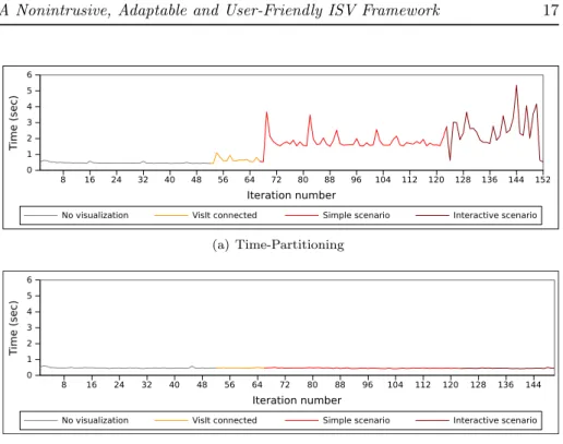
In each case, we consider four scenarios: (A) the simulation runs without visualization, (B) a user connects VisIt to the simulation but does not ask for any output,(C) the user asks for iso-surfaces of the velocity fields but does not interact with VisIt any further (letting the simulation update the output after each iteration) and finally (D) the user has heavy interactions with the simulations (rendering different variables, using different algorithms, zooming on particular domains, changing the resolution, etc).
5.2.3 Results with the TurbChannel configuration
Figure 5 presents a trace of the duration of each iteration during the four afore-mentioned scenarios using the two approaches. The top graph in Figure 5 shows that ISV using a time-partitioning approach has a negative impact on the sim-ulation run time, even when no interaction is performed. Space-partitioning ISV, on the other hand, is completely transparent from the point of view of the simulation.
8 16 24 32 40 48 56 64 72 80 88 96 104 112 120 128 136 144 152 Iteration number 0 1 2 3 4 5 6 T ime (sec)
No visualization VisIt connected Simple scenario Interactive scenario
(a) Time-Partitioning 8 16 24 32 40 48 56 64 72 80 88 96 104 112 120 128 136 144 Iteration number 0 1 2 3 4 5 6 T ime (sec)
No visualization VisIt connected Simple scenario Interactive scenario
(b) Space-Partitioning
Figure 5: Variability in run-time induced by different scenarios of in situ inter-active visualization.
Iteration time Average Std. dev.
Time-partitioning no vis.with vis. 205.21 sec75.07 sec 22,9357.15 Space-partitioning no vis.with vis. 67.76 sec64.79 sec 20.0920.44
Table 2: Average iteration time of the Nek5000 MATiS configuration with time-partitioning and space-time-partitioning approaches, with and without visualization. 5.2.4 Experiments with the MATiS configuration
The MATiS configuration requires a larger scale; we ran it on 816 cores. Each iteration taking approximately one minute and due to the huge number of points that the mesh contains, it is difficult to perform interactive visualization. We therefore connect VisIt and simply query for a 3D pseudo-color plot of the vx variable.
5.2.5 Results with the MATiS configuration
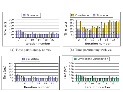
Figure 6 reports the behavior of the application with and without visualization performed, and with and without dedicated cores. Corresponding statistics are presented in Table 2.
Time-partitioning visualization not only increases the average run time but also increases the standard deviation, making run times unpredictable. On the other hand, the space-partitioning yields excellent results. Intuitively, we expect
2 6 10 14 18 22 Iteration number 0 50 100 150 200 250 300 T ime (sec) Simulation
(a) Time-partitioning, no vis.
2 6 10 14 18 22 Iteration number 0 50 100 150 200 250 300 T ime (sec) Visualization Simulation
(b) Time-partitioning with vis.
2 6 10 14 18 22 Iteration number 0 50 100 150 200 250 300 T ime (sec) Simulation (c) Space-partitioning, no vis. 2 6 10 14 18 22 Iteration number 0 50 100 150 200 250 300 T ime (sec) Simulation+Visualization
(d) Space-partitioning with vis.
Figure 6: Iteration time of the MATiS configuration without visualization (left) and with visualization enabled (right). Top: With time-partitioning, tion time adds to simulation time. Bottom: With space-partitioning, visualiza-tion time is entirely overlapped with simulavisualiza-tion time.
a space-partitioning approach to interfere with the simulation, as it performs intensive communications while the simulation runs. However, in practice we observe very little run time variation.
While the time-partitioning approach performs visualization at every time step, the space-partitioning approach has adapted the frequency of its output to 1 frame every 25 time steps (an acceptable number for Nek5000 users). If a time-partitioning approach were to only output 1 frame every 25 time steps, the completion time for 25 time steps would be 2007 seconds on average. With space-partitioning in Damaris/Viz this takes 1620 seconds, a 20% speedup. Fur-thermore, since space-partitioning in Damaris overlaps the visualization and simulation, the total run time is unchanged with the addition of ISV.
6
Conclusion and future work
The slower rate at which I/O performance is increasing compared to that of computational capabilities necessitates new approaches for gaining insights from running simulations. Tightly-coupled in situ visualization appears to be a viable approach to reduce the pressure on file systems. Yet the synchronous aspect of existing solutions and the impact on the simulation’s performance has limited its adoption in the HPC community.
We proposed Damaris/Viz, an in situ visualization framework based on the Damaris I/O middleware. By leveraging dedicated cores, external high-level structure description and a simple API, our framework provides adaptable in
situ visualization to existing simulations at a low instrumentation cost. Results obtained with the Nek5000 CFD and CM1 atmospheric simulations show that our framework can completely hide the performance impact of visualization tasks. In addition, the proposed API allows efficient memory usage through a shared memory, zero-copy communication model.
As future works, we plan to evaluate our framework more extensively on heterogeneous architectures. Additionally, we plan to improve our framework to be able to utilize a set of dedicated nodes (in a loosely-coupled model), and to choose the level of coupling at run time depending on resource usage in the simulation, I/O bandwidth availability, the presence of accelerators and temporary storage devices.
Acknowledgments
This work was a collaboration between the KerData INRIA - ENS Cachan/Brittany team (Rennes, France), the NCSA (Urbana-Champaign, USA) and ANL within the Joint INRIA-UIUC-ANL Laboratory for Petascale Computing. The experiments were carried out using the Grid’5000/ ALADDIN-G5K experimental testbed (see http: //www.grid5000.fr/) and Blue Waters at NCSA (see http://www.ncsa.illinois. edu/BlueWaters/). We thank Leigh Orf for his insights on the CM1 application and the datasets he provided for our experiments, Paul Fischer and Aleksandr Obabko for providing insights and datasets for Nek5000, and Shadi Ibrahim for his feedbacks on this paper. We also acknowledge the VisIt developers, in particular Hank Childs, Brad Whitlock and Jean Favre for their help with using VisIt’s in situ interface.
References
[1] G. H. Bryan and J. M. Fritsch. A Benchmark Simulation for Moist Nonhydrostatic Numerical Models. Monthly Weather Review, 130(12):2917–2928, 2002.
[2] H. Childs, D. Pugmire, S. Ahern, B. Whitlock, M. Howison, Prabhat, G. Weber, and E. Bethel. Extreme Scaling of Production Visualization Software on Diverse Architectures. Computer Graphics and Applications, IEEE, 30(3):22–31, may-june 2010.
[3] M. Dorier. Src: Damaris - using dedicated i/o cores for scalable post-petascale hpc simulations. In Proceedings of the international conference on Supercomputing, ICS ’11, pages 370–370, New York, NY, USA, 2011. ACM.
[4] M. Dorier, G. Antoniu, F. Cappello, M. Snir, and L. Orf. Damaris: Leveraging Multicore Parallelism to Mask I/O Jitter. Research report RR-7706, INRIA, Dec. 2011.
[5] M. Dorier, G. Antoniu, F. Cappello, M. Snir, and L. Orf. Damaris: How to efficiently leverage multicore parallelism to achieve scalable, jitter-free i/o. In Cluster Computing (CLUSTER), 2012 IEEE International Conference on, pages 155 –163, sept. 2012.
[6] D. Ellsworth, B. Green, C. Henze, P. Moran, and T. Sandstrom. Concurrent Visualization in a Production Supercomputing Environment. Visualization and Computer Graphics, IEEE Transactions on, 12(5):997 –1004, sept.-oct. 2006. [7] A. Esnard, N. Richart, and O. Coulaud. A steering environment for online parallel
visualization of legacy parallel simulations. In Distributed Simulation and Real-Time Applications, 2006. DS-RT’06. Tenth IEEE International Symposium on, pages 7–14. IEEE, 2006.
[8] EzViz. http://www.ezviz.biz/.
[9] N. Fabian, K. Moreland, D. Thompson, A. Bauer, P. Marion, B. Geveci, M. Rasquin, and K. Jansen. The ParaView Coprocessing Library: A Scalable, General Purpose In Situ Visualization Library. In LDAV, IEEE Symposium on Large-Scale Data Analysis and Visualization, 2011.
[10] A. Geist and R. Lucas. Major Computer Science Challenges At Exascale. Inter-national Journal of High Performance Computing Applications, 23(4):427–436, 2009.
[11] A. Hoisie and V. Getov. Extreme-Scale Computing - Where ’Just More of the Same’ Does Not Work. Computer, 42(11):24–26, nov. 2009.
[12] INRIA. Aladdin grid’5000: http://www.grid5000.fr.
[13] C. Johnson, S. Parker, C. Hansen, G. Kindlmann, and Y. Livnat. Interactive simulation and visualization. Computer, 32(12):59–65, 1999.
[14] KerData, IRISA, INRIA Rennes. Damaris, http://damaris.gforge.inria.fr/. [15] KitWare. ParaView, http://www.paraview.org/.
[16] M. Li, S. S. Vazhkudai, A. R. Butt, F. Meng, X. Ma, Y. Kim, C. Engelmann, and G. Shipman. Functional Partitioning to Optimize End-to-End Performance on Many-core Architectures. In Proceedings of the 2010 ACM/IEEE International Conference for High Performance Computing, Networking, Storage and Analysis, SC ’10, pages 1–12, Washington, DC, USA, 2010. IEEE Computer Society. [17] LLNL. VisIt, https://wci.llnl.gov/codes/visit/.
[18] J. Lofstead, F. Zheng, Q. Liu, S. Klasky, R. Oldfield, T. Kordenbrock, K. Schwan, and M. Wolf. Managing Variability in the IO Performance of Petascale Storage Systems. In Proceedings of the 2010 ACM/IEEE International Conference for High Performance Computing, Networking, Storage and Analysis, SC ’10, pages 1–12, Washington, DC, USA, 2010. IEEE Computer Society.
[19] J. F. Lofstead, S. Klasky, K. Schwan, N. Podhorszki, and C. Jin. Flexible IO and integration for scientific codes through the adaptable IO system (ADIOS). In Proceedings of the 6th international workshop on Challenges of large applications in distributed environments, CLADE ’08, pages 15–24, New York, NY, USA, 2008. ACM.
[20] X. Ma, J. Lee, and M. Winslett. High-level buffering for hiding periodic output cost in scientific simulations. Parallel and Distributed Systems, IEEE Transac-tions on, 17(3):193–204, 2006.
[21] P. Malakar, V. Natarajan, and S. S. Vadhiyar. An Adaptive Framework for Simulation and Online Remote Visualization of Critical Climate Applications in Resource-constrained Environments. In Proceedings of the 2010 ACM/IEEE International Conference for High Performance Computing, Networking, Storage and Analysis, SC ’10, pages 1–11, Washington, DC, USA, 2010. IEEE Computer Society.
[22] K. Moreland, R. Oldfield, P. Marion, S. Jourdain, N. Podhorszki, V. Vishwanath, N. Fabian, C. Docan, M. Parashar, M. Hereld, et al. Examples of in transit visualization. In Proceedings of the 2nd international workshop on Petascal data analytics: challenges and opportunities, pages 1–6. ACM, 2011.
[23] NCSA. BlueWaters project, http://www.ncsa.illinois.edu/BlueWaters/. [24] J. W. L. Paul F. Fischer and S. G. Kerkemeier. nek5000 Web page, 2008.
[25] M. Rasquin, P. Marion, V. Vishwanath, B. Matthews, M. Hereld, K. Jansen, R. Loy, A. Bauer, M. Zhou, O. Sahni, et al. Electronic poster: co-visualization of full data and in situ data extracts from unstructured grid cfd at 160k cores. In Proceedings of the 2011 companion on High Performance Computing Networking, Storage and Analysis Companion, pages 103–104. ACM, 2011.
[26] M. Rivi, L. Calori, G. Muscianisi, and V. Slavnic. In-Situ Visualization: State-of-the-art and Some Use Cases.
[27] W. Schroeder, L. Avila, and W. Hoffman. Visualizing with VTK: a tutorial. Computer Graphics and Applications, IEEE, 20(5):20 –27, sep/oct 2000. [28] D. Skinner and W. Kramer. Understanding the causes of performance variability
in HPC workloads. In Workload Characterization Symposium, 2005. Proceedings of the IEEE International, pages 137 – 149, oct. 2005.
[29] D. Thompson, N. Fabian, K. Moreland, and L. Ice. Design issues for performing in situ analysis of simulation data. Technical report, Technical Report SAND2009-2014, Sandia National Laboratories, 2009.
[30] T. Tu, H. Yu, L. Ramirez-Guzman, J. Bielak, O. Ghattas, K.-L. Ma, and D. R. O’Hallaron. From mesh generation to scientific visualization: an end-to-end ap-proach to parallel supercomputing. In Proceedings of the 2006 ACM/IEEE con-ference on Supercomputing, SC ’06, New York, NY, USA, 2006. ACM.
[31] M. J. Turk, B. D. Smith, J. S. Oishi, S. Skory, S. W. Skillman, T. Abel, and M. L. Norman. yt: A Multi-code Analysis Toolkit for Astrophysical Simulation Data. The Astrophysical Journal Supplement Series, 192(1):9, 2011.
[32] B. Whitlock, J. M. Favre, and J. S. Meredith. Parallel In Situ Coupling of Simula-tion with a Fully Featured VisualizaSimula-tion System. In Eurographics Symposium on Parallel Graphics and Visualization (EGPGV). Eurographics Association, 2011. [33] H. Yu and K.-L. Ma. A study of I/O methods for parallel visualization of
large-scale data. Parallel Computing, 31(2):167 – 183, 2005. Parallel Graphics and Visualization.
[34] F. Zhang, C. Docan, M. Parashar, S. Klasky, N. Podhorszki, and H. Abbasi. Enabling in-situ execution of coupled scientific workflow on multi-core platform. Parallel and Distributed Processing Symposium, International, 0:1352–1363, 2012. [35] F. Zhang, S. Lasluisa, T. Jin, I. Rodero, H. Bui, and M. Parashar. In-situ
feature-based objects tracking for large-scale scientific simulations. In DISCS, 2012. [36] F. Zheng, H. Abbasi, J. Cao, J. Dayal, K. Schwan, M. Wolf, S. Klasky, and
N. Podhorszki. In-situ i/o processing: A case for location flexibility. simulation, 25:28, 2011.
[37] F. Zheng, H. Abbasi, C. Docan, J. Lofstead, Q. Liu, S. Klasky, M. Parashar, N. Podhorszki, K. Schwan, and M. Wolf. PreDatA - preparatory data analytics on peta-scale machines. In Parallel Distributed Processing (IPDPS), 2010 IEEE International Symposium on, pages 1 –12, april 2010.
// This f u n c t i o n i s c a l l e d to r e t r i e v e the mesh
v i s i t _ h a n d l e get_mesh_data (i n t domain ,
const char ∗name , void ∗ cbdata ) { v i s i t _ h a n d l e h = VISIT_INVALID_HANDLE;
i f( strcmp (name , "my_mesh") == 0) {
i f( Vis It_R ecti l i ne arMesh_alloc (&h ) == VISIT_OKAY) {
v i s i t _ h a n d l e hxc , hyc , hzc ; VisIt_VariableData_alloc (&hxc ) ;
// . . . idem f o r hyc and hzc
VisIt_VariableData_setDataF ( hxc , VISIT_OWNER_SIM, 1 , NX, mesh_x ) ;
// . . . idem f o r hyc and hzc
VisIt_RectilinearMesh_setCoordsXYZ (h , hxc , hyc , hzc ) ; } } r e t u r n h ; } }
// This f u n c t i o n i s c a l l e d to r e t r i e v e the data
v i s i t _ h a n d l e get_variable_data (i n t domain ,
const char ∗name , void ∗ cbdata ) { v i s i t _ h a n d l e h = VISIT_INVALID_HANDLE; i f( strcmp (name , " temperature ") == 0) { i f( VisIt_VariableData_alloc (&h ) == VISIT_OKAY) { i n t s i z e = NX∗NY∗NZ; VisIt_VariableData_setDataD (h , VISIT_OWNER_SIM, 1 , s i z e , temp ) ; } } r e t u r n h ; }
// When a V i s I t c l i e n t connects , the c a l l b a c k // f u n c t i o n s has to be provided using
VisItSetGetMesh ( get_mesh_data ,NULL) ;
V i s I t S e t G e t V a r i a b l e ( get_variable_data ,NULL) ;
Listing 4: Data access functions for our sample application using VisIt. The first function retrieves the mesh coordinates, while the second retrieves the temperature field. The two last lines register the two functions as callbacks handling data accesses. This sample code does not show the modifications to perform in the simulation’s main loop.
// Create the v a r i a b l e data vtkDataArray ∗ wrapMyData ( . . . ) { vtkDoubleArray ∗ myArray = vtkDoubleArray : : New ( ) ; myArray−>SetName (" temperature ") ; vtkIdType s i z e = NX∗NY∗NZ; myArray−>SetArray ( temp , s i z e , 1 ) ; r e t u r n myArray ; }
// This f u n c t i o n i s c a l l e d to r e t r i e v e the mesh
vtkObject ∗ wrapMeshData ( . . . ) {
// c r e a t e s the n e c e s s a r y c o o r d i n a t e a r r a y s
vtkFloatArray ∗ xCoords , yCoords , zCoords ; xCoords = vtkFloatArray : : New ( ) ;
xCoords−>setArray (mesh_x ,PTX, 1 ) ;
// . . . idem f o r yCoords and zCoords
v t k R e c t i l i n e a r G r i d ∗ g r i d
= v t k R e c t i l i n e a r G r i d : : New ( ) ; grid −>setDimensions (NX,NY,NZ ) ; grid −>setXCoordinates ( xCoords ) ;
// . . . idem f o r Y and Z c o o r d i n a t e s
vtkDataArray ∗ array
= wrapMyData ( ) ; // s e e above
grid −>GetPointData()−>AddArray ( array ) ; array−>Delete ( ) ;
r e t u r n ( vtkObject ∗) g r i d ; }
Listing 5: Data access functions for our sample application using ParaView. The first function wraps the temperature field into the VTK object which is used by the second function that adds information related to the mesh coordinates.